
CHAPTER SEVENTEEN
Graph Properties and Types
MANY COMPUTATIONAL APPLICATIONS naturally involve not just a set of items, but also a set of connections between pairs of those items. The relationships implied by these connections lead immediately to a host of natural questions: Is there a way to get from one item to another by following the connections? How many other items can be reached from a given item? What is the best way to get from this item to this other item?
To model such situations, we use abstract objects called graphs. In this chapter, we examine basic properties of graphs in detail, setting the stage for us to study a variety of algorithms that are useful for answering questions of the type just posed. These algorithms make effective use of many of the computational tools that we considered in Parts 1 through 4. They also serve as the basis for attacking problems in important applications whose solution we could not even contemplate without good algorithmic technology.
Graph theory, a major branch of combinatorial mathematics, has been studied intensively for hundreds of years. Many important and useful properties of graphs have been proved, yet many difficult problems remain unresolved. In this book, while recognizing that there is much still to be learned, we draw from this vast body of knowledge about graphs what we need to understand and use a broad variety of useful and fundamental algorithms.
Like so many of the other problem domains that we have studied, the algorithmic investigation of graphs is relatively recent. Although a few of the fundamental algorithms are old, the majority of the interesting ones have been discovered within the last few decades. Even the simplest graph algorithms lead to useful computer programs, and the nontrivial algorithms that we examine are among the most elegant and interesting algorithms known.
To illustrate the diversity of applications that involve graph processing, we begin our exploration of algorithms in this fertile area by considering several examples.
Maps A person who is planning a trip may need to answer questions such as, “What is the least expensive way to get from Princeton to San Jose?” A person more interested in time than in money may need to know the answer to the question “What is the fastest way to get from Princeton to San Jose?” To answer such questions, we process information about connections (travel routes) between items (towns and cities).
Hypertexts When we browse the Web, we encounter documents that contain references (links) to other documents, and we move from document to document by clicking on the links. The entire web is a graph, where the items are documents and the connections are links. Graph-processing algorithms are essential components of the search engines that help us locate information on the web.
Circuits An electric circuit comprises elements such as transistors, resistors, and capacitors that are intricately wired together. We use computers to control machines that make circuits, and to check that the circuits perform desired functions. We need to answer simple questions such as, “Is a short-circuit present?” as well as complicated questions such as, “Can we lay out this circuit on a chip without making any wires cross?” In this case, the answer to the first question depends on only the properties of the connections (wires), whereas the answer to the second question requires detailed information about the wires, the items that those wires connect, and the physical constraints of the chip.
Schedules A manufacturing process requires a variety of tasks to be performed, under a set of constraints that specifies that certain tasks cannot be started until certain other tasks have been completed. We represent the constraints as connections between the tasks (items), and we are faced with a classical scheduling problem: How do we schedule the tasks such that we both respect the given constraints and complete the whole process in the least amount of time?
Transactions A telephone company maintains a database of telephone-call traffic. Here the connections represent telephone calls. We are interested in knowing about the nature of the interconnection structure because we want to lay wires and build switches that can handle the traffic efficiently. As another example, a financial institution tracks buy/sell orders in a market. A connection in this situation represents the transfer of cash between two customers. Knowledge of the nature of the connection structure in this instance may enhance our understanding of the nature of the market.
Matching Students apply for positions in selective institutions such as social clubs, universities, or medical schools. Items correspond to the students and the institutions; connections correspond to the applications. We want to discover methods for matching interested students with available positions.
Networks A computer network consists of interconnected sites that send, forward, and receive messages of various types. We are interested not just in knowing that it is possible to get a message from every site to every other site, but also in maintaining this connectivity for all pairs of sites as the network changes. For example, we might wish to check a given network to be sure that no small set of sites or connections is so critical that losing it would disconnect any remaining pair of sites.
Program structure A compiler builds graphs to represent the call structure of a large software system. The items are the various functions or modules that comprise the system; connections are associated either with the possibility that one function might call another (static analysis) or with actual calls while the system is in operation (dynamic analysis). We need to analyze the graph to determine how best to allocate resources to the program most efficiently.
These examples indicate the range of applications for which graphs are the appropriate abstraction and also the range of computational problems that we might encounter when we work with graphs. Such problems will be our focus in this book. In many of these applications as they are encountered in practice, the volume of data involved is truly huge, and efficient algorithms make the difference between whether or not a solution is at all feasible.
We have already encountered graphs, briefly, in Part 1. Indeed, the first algorithms that we considered in detail, the union-find algorithms in Chapter 1, are prime examples of graph algorithms. We also used graphs in Chapter 3 as an illustration of applications of two-dimensional arrays and linked lists, and in Chapter 5 to illustrate the relationship between recursive programs and fundamental data structures. Any linked data structure is a representation of a graph, and some familiar algorithms for processing trees and other linked structures are special cases of graph algorithms. The purpose of this chapter is to provide a context for developing an understanding of graph algorithms ranging from the simple ones in Part 1 to the sophisticated ones in Chapters 18 through 22.
As always, we are interested in knowing which are the most efficient algorithms that solve a particular problem. The study of the performance characteristics of graph algorithms is challenging because
• The cost of an algorithm depends not just on properties of the set of items, but also on numerous properties of the set of connections (and global properties of the graph that are implied by the connections).
• Accurate models of the types of graphs that we might face are difficult to develop.
We often work with worst-case performance bounds on graph algorithms, even though they may represent pessimistic estimates on actual performance in many instances. Fortunately, as we shall see, a number of algorithms are optimal and involve little unnecessary work. Other algorithms consume the same resources on all graphs of a given size. We can predict accurately how such algorithms will perform in specific situations. When we cannot make such accurate predictions, we need to pay particular attention to properties of the various types of graphs that we might expect in practical applications and must assess how these properties might affect the performance of our algorithms.
We begin by working through the basic definitions of graphs and the properties of graphs, examining the standard nomenclature that is used to describe them. Following that, we define the basic ADT (abstract data type) interfaces that we use to study graph algorithms and the two most important data structures for representing graphs—the adjacency-matrix representation and the adjacency-lists representation, and various approaches to implementing basic ADT functions. Then, we consider client programs that can generate random graphs, which we can use to test our algorithms and to learn properties of graphs. All this material provides a basis for us to introduce graph-processing algorithms that solve three classical problems related to finding paths in graphs, which illustrate that the difficulty of graph problems can differ dramatically even when they might seem similar. We conclude the chapter with a review of the most important graph-processing problems that we consider in this book, placing them in context according to the difficulty of solving them.
17.1 Glossary
A substantial amount of nomenclature is associated with graphs. Most of the terms have straightforward definitions, and, for reference, it is convenient to consider them in one place: here. We have already used some of these concepts when considering basic algorithms in Part 1; others of them will not become relevant until we address associated advanced algorithms in Chapters 18 through 22.
Definition 17.1 A graph is a set of vertices and a set of edges that connect pairs of distinct vertices (with at most one edge connecting any pair of vertices).
We use the names 0 through V-1 for the vertices in a V -vertex graph. The main reason that we choose this system is that we can access quickly information corresponding to each vertex, using vector indexing. In Section 17.6, we consider a program that uses a symbol table to establish a 1–1 mapping to associate V arbitrary vertex names with the V integers between 0 and V − 1. With that program in hand, we can use indices as vertex names (for notational convenience) without loss of generality. We sometimes assume that the set of vertices is defined implicitly, by taking the set of edges to define the graph and considering only those vertices that are included in at least one edge. To avoid cumbersome usage such as “the ten-vertex graph with the following set of edges,” we do not explicitly mention the number of vertices when that number is clear from the context. By convention, we always denote the number of vertices in a given graph by V, and denote the number of edges by E.
We adopt as standard this definition of a graph (which we first encountered in Chapter 5), but note that it embodies two technical simplifications. First, it disallows duplicate edges (mathematicians sometimes refer to such edges as parallel edges, and a graph that can contain them as a multigraph). Second, it disallows edges that connect vertices to themselves; such edges are called self-loops. Graphs that have no parallel edges or self-loops are sometimes referred to as simple graphs.
We use simple graphs in our formal definitions because it is easier to express their basic properties and because parallel edges and self-loops are not needed in many applications. For example, we can bound the number of edges in a simple graph with a given number of vertices.
Property 17.1 Agraphwith V vertices has at most V (V − 1)/ 2 edges.
Proof: The total of V2 possible pairs of vertices includes V self-loops and accounts twice for each edge between distinct vertices, so the number of edges is at most (V2 − V)/2=V (V − 1)/2. •
No such bound holds if we allow parallel edges: a graph that is not simple might consist of two vertices and billions of edges connecting them (or even a single vertex and billions of self-loops).
For some applications, we might consider the elimination of parallel edges and self-loops to be a data-processing problem that our implementations must address. For other applications, ensuring that a given set of edges represents a simple graph may not be worth the trouble. Throughout the book, whenever it is more convenient to address an application or to develop an algorithm by using an extended definition that includes parallel edges or self-loops, we shall do so. For example, self-loops play a critical role in a classical algorithm that we will examine in Section 17.4; and parallel edges are common in the applications that we address in Chapter 22. Generally, it is clear from the context whether we intend the term “graph” to mean “simple graph” or “multigraph” or “multigraph with self-loops.”
Mathematicians use the words vertex and node interchangeably, but we generally use vertex when discussing graphs and node when discussing representations—for example, in C++ data structures. We normally assume that a vertex can have a name and can carry other associated information. Similarly, the words arc, edge, and link are all widely used by mathematicians to describe the abstraction embodying a connection between two vertices, but we consistently use edge when discussing graphs and link when discussing C++ data structures.
When there is an edge connecting two vertices, we say that the vertices are adjacent to one another and that the edge is incident on both vertices. The degree of a vertex is the number of edges incident on it. We use the notation v-w to represent an edge that connects v and w; the notation w-v is an alternative way to represent the same edge.
A subgraph is a subset of a graph’s edges (and associated vertices) that constitutes a graph. Many computational tasks involve identifying subgraphs of various types. If we identify a subset of a graph’s vertices, we call that subset, together with all edges that connect two of its members, the induced subgraph associated with those vertices.
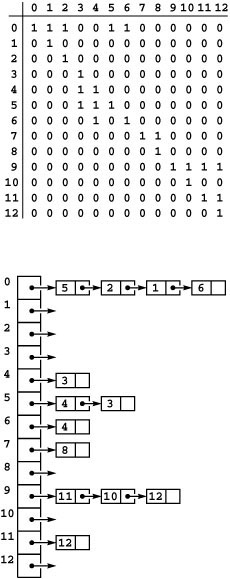
We can draw a graph by marking points for the vertices and drawing lines connecting them for the edges. A drawing gives us intuition about the structure of the graph; but this intuition can be misleading, because the graph is defined independently of the representation. For example, the two drawings in Figure 17.1 and the list of edges represent the same graph, because the graph is only its (unordered) set of vertices and its (unordered) set of edges (pairs of vertices)—nothing more. Although it suffices to consider a graph simply as a set of edges, we examine other representations that are particularly suitable as the basis for graph data structures in Section 17.4.
Figure 17.1 Three different representations of the same graph
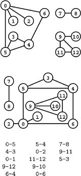
A graph is defined by its vertices and its edges, not by the way that we choose to draw it. These two drawings depict the same graph, as does the list of edges (bottom), given the additional information that the graph has 13 vertices labeled 0 through 12.
Placing the vertices of a given graph on the plane and drawing them and the edges that connect them is known as graph drawing. The possible vertex placements, edge-drawing styles, and aesthetic constraints on the drawing are limitless. Graph-drawing algorithms that respect various natural constraints have been studied heavily and have many successful applications (see reference section). For example, one of the simplest constraints is to insist that edges do not intersect. A planar graph is one that can be drawn in the plane without any edges crossing. Determining whether or not a graph is planar is a fascinating algorithmic problem that we discuss briefly in Section 17.8. Being able to produce a helpful visual representation is a useful goal, and graph drawing is a fascinating field of study, but successful drawings are often difficult to realize. Many graphs that have huge numbers of vertices and edges are abstract objects for which no suitable drawing is feasible.
For some applications, such as graphs that represent maps or circuits, a graph drawing can carry considerable information because the vertices correspond to points in the plane and the distances between them are relevant. We refer to such graphs as Euclidean graphs. For many other applications, such as graphs that represent relationships or schedules, the graphs simply embody connectivity information, and no particular geometric placement of vertices is ever implied. We consider examples of algorithms that exploit the geometric information in Euclidean graphs in Chapters 20 and 21, but we primarily work with algorithms that make no use of any geometric information, and stress that graphs are generally independent of any particular representation in a drawing or in a computer.
Focusing solely on the connections themselves, we might wish to view the vertex labels as merely a notational convenience, and to regard two graphs as being the same if they differ in only the vertex labels. Two graphs are isomorphic if we can change the vertex labels on one to make its set of edges identical to the other. Determining whether or not two graphs are isomorphic is a difficult computational problem (see Figure 17.2 and Exercise 17.5). It is challenging because there are V ! possible ways to label the vertices—far too many for us to try all the possibilities. Therefore, despite the potential appeal of reducing the number of different graph structures that we have to consider by treating isomorphic graphs as identical structures, we rarely do so.
As we saw with trees in Chapter 5, we are often interested in basic structural properties that we can deduce by considering specific sequences of edges in a graph.
Definition 17.2 A path in a graph is a sequence of vertices in which each successive vertex (after the first) is adjacent to its predecessor in the path. In a simple path , the vertices and edges are distinct. A cycle is a path that is simple except that the first and final vertices are the same.
Figure 17.2 Graph isomorphism examples

The top two graphs are isomorphic because we can relabel the vertices to make the two sets of edges identical (to make the middle graph the same as the top graph, change 10 to 4, 7 to 3, 2 to 5, 3 to 1, 12 to 0, 5 to 2, 9 to 11, 0 to 12, 11 to 9, 1 to 7, and 4 to 10). The bottom graph is not isomorphic to the others because there is no way to relabel the vertices to make its set of edges identical to either.
We sometimes use the term cyclic path to refer to a path whose first and final vertices are the same (and is otherwise not necessarily simple); and we use the term tour to refer to a cyclic path that includes every vertex. An equivalent way to define a path is as the sequence of edges that connect the successive vertices. We emphasize this in our notation by connecting vertex names in a path in the same way as we connect them in an edge. For example, the simple paths in Figure 17.1 include 3-4-6-0-2, and 9-12-11, and the cycles in the graph include 0-6-4-3-5-0 and 5-4-3-5. We define the length of a path or a cycle to be its number of edges.
Figure 17.3 Graph terminology
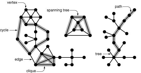
This graph has 55 vertices, 70 edges, and 3 connected components. One of the connected components is a tree (right). The graph has many cycles, one of which is highlighted in the large connected component (left). The diagram also depicts a spanning tree in the small connected component (center). The graph as a whole does not have a spanning tree, because it is not connected.
We adopt the convention that each single vertex is a path of length 0 (a path from the vertex to itself with no edges on it, which is different from a self-loop). Apart from this convention, in a graph with no parallel edges and no self-loops, a pair of vertices uniquely determines an edge, paths must have on them at least two distinct vertices, and cycles must have on them at least three distinct edges and three distinct vertices.
We say that two simple paths are disjoint if they have no vertices in common other than, possibly, their endpoints. Placing this condition is slightly weaker than insisting that the paths have no vertices at all in common, and is useful because we can combine simple disjoint paths from s to t and t to u to get a simple disjoint path from s to u if s and u are different (and to get a cycle if s and u are the same). The term vertex disjoint is sometimes used to distinguish this condition from the stronger condition of edge disjoint, where we require that the paths have no edge in common.
Definition 17.3 A graph is a connected graph if there is a path from every vertex to every other vertex in the graph. A graph that is not connected consists of a set of connected components , which are maximal connected subgraphs.
The term maximal connected subgraph means that there is no path from a subgraph vertex to any vertex in the graph that is not in the subgraph. Intuitively, if the vertices were physical objects, such as knots or beads, and the edges were physical connections, such as strings or wires, a connected graph would stay in one piece if picked up by any vertex, and a graph that is not connected comprises two or more such pieces.
Definition 17.4 An acyclic connected graph is called a tree (see Chapter 4). A set of trees is called a forest . A spanning tree of a connected graph is a subgraph that contains all of that graph’s vertices and is a single tree. A spanning forest of a graph is a subgraph that contains all of that graph’s vertices and is a forest.
For example, the graph illustrated in Figure 17.1 has three connected components, and is spanned by the forest 7-8 9-10 9-11 9-12 0-1 0-2 0-5 5-3 5-4 4-6 (there are many other spanning forests). Figure 17.3 highlights these and other features in a larger graph.
We explore further details about trees in Chapter 4, and look at various equivalent definitions. For example, a graph G with V vertices is a tree if and only if it satisfies any of the following four conditions:
• G has V − 1 edges and no cycles.
• G has V − 1 edges and is connected.
• Exactly one simple path connects each pair of vertices in G.
• G is connected, but removing any edge disconnects it.
Any one of these conditions is necessary and sufficient to prove the other three, and we can develop other combinations of facts about trees from them (see Exercise 17.1). Formally, we should choose one condition to serve as a definition; informally, we let them collectively serve as the definition, and freely engage in usage such as the “acyclic connected graph” choice in Definition 17.4.
Graphs with all edges present are called complete graphs (see Figure 17.4). We define the complement of a graph G by starting with a complete graph that has the same set of vertices as the original graph and then removing the edges of G. The union of two graphs is the graph induced by the union of their sets of edges. The union of a graph and its complement is a complete graph. All graphs that have V vertices are subgraphs of the complete graph that has V vertices. The total number of different graphs that have V vertices is 2V (V −1)/2 (the number of different ways to choose a subset from the V (V - 1)/2 possible edges). A complete subgraph is called a clique.
Figure 17.4 Complete graphs
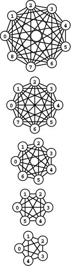
These complete graphs, with every vertex connected to every other vertex, have 10, 15, 21, 28, and 36 edges (bottom to top). Every graph with between 5 and 9 vertices (there are more than 68 billion such graphs) is a subgraph of one of these graphs.
Most graphs that we encounter in practice have relatively few of the possible edges present. To quantify this concept, we define the density of a graph to be the average vertex degree, or 2E/V. A dense graph is a graph whose average vertex degree is proportional to V; a sparse graph is a graph whose complement is dense. In other words, we consider a graph to be dense if E is proportional to V2 and sparse otherwise. This asymptotic definition is not necessarily meaningful for a particular graph, but the distinction is generally clear: A graph that has millions of vertices and tens of millions of edges is certainly sparse, and a graph that has thousands of vertices and millions of edges is certainly dense. We might contemplate processing a sparse graph with billions of vertices, but a dense graph with billions of vertices would have an overwhelming number of edges.
Knowing whether a graph is sparse or dense is generally a key factor in selecting an efficient algorithm to process the graph. For example, for a given problem, we might develop one algorithm that takes about V2 steps and another that takes about E lg E steps. These formulas tell us that the second algorithm would be better for sparse graphs, whereas the first would be preferred for dense graphs. For example, a dense graph with millions of edges might have only thousands of vertices: in this case V2 and E would be comparable in value, and the V2 algorithm would be 20 times faster than the E lg E algorithm. On the other hand, a sparse graph with millions of edges also has millions of vertices, so the E lg E algorithm could be millions of times faster than the V2 algorithm. We could make specific tradeoffs on the basis of analyzing these formulas in more detail, but it generally suffices in practice to use the terms sparse and dense informally to help us understand fundamental performance characteristics.
When analyzing graph algorithms, we assume that V/E is bounded above by a small constant, so that we can abbreviate expressions such as V (V + E ) to V E. This assumption comes into play only when the number of edges is tiny in comparison to the number of vertices—a rare situation. Typically, the number of edges far exceeds the number of vertices (V/E is much less than 1).
A bipartite graph is a graph whose vertices we can divide into two sets such that all edges connect a vertex in one set with a vertex in the other set. Figure 17.5 gives an example of a bipartite graph. Bipartite graphs arise in a natural way in many situations, such as the matching problems described at the beginning of this chapter. Any subgraph of a bipartite graph is bipartite.
Figure 17.5 A bipartite graph
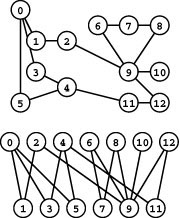
All edges in this graph connect odd-numbered vertices with even-numbered ones, so it is bipartite. The bottom diagram makes the property obvious.
Graphs as defined to this point are called undirected graphs. In directed graphs, also known as digraphs, edges are one-way: we consider the pair of vertices that defines each edge to be an ordered pair that specifies a one-way adjacency where we think about having the ability to get from the first vertex to the second but not from the second vertex to the first. Many applications (for example, graphs that represent the Web, scheduling constraints, or telephone-call transactions) are naturally expressed in terms of digraphs.
We refer to edges in digraphs as directed edges, though that distinction is generally obvious in context (some authors reserve the term arc for directed edges). The first vertex in a directed edge is called the source; the second vertex is called the destination. (Some authors use the terms tail and head, respectively, to distinguish the vertices in directed edges, but we avoid this usage because of overlap with our use of the same terms in data-structure implementations.) We draw directed edges as arrows pointing from source to destination, and often say that the edge points to the destination. When we use the notation v-w in a digraph, we mean it to represent an edge that points from v to w; it is different from w-v, which represents an edge that points from w to v. We speak of the indegree and outdegree of a vertex (the number of edges where it is the destination and the number of edges where it is the source, respectively).
Sometimes, we are justified in thinking of an undirected graph as a digraph that has two directed edges (one in each direction); other times, it is useful to think of undirected graphs simply in terms of connections. Normally, as discussed in detail in Section 17.4, we use the same representation for directed and undirected graphs (see Figure 17.6). That is, we generally maintain two representations of each edge for undirected graphs, one pointing in each direction, so that we can immediately answer questions such as, “Which vertices are connected to vertex v?”
Figure 17.6 Two digraphs
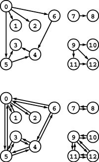
The drawing at the top is a representation of the example graph in Figure 17.1 interpreted as a directed graph, where we take the edges to be ordered pairs and represent them by drawing an arrow from the first vertex to the second. It is also a DAG. The drawing at the bottom is a representation of the undirected graph from Figure 17.1 that indicates the way that we usually represent undirected graphs: as digraphs with two edges corresponding to each connection (one in each direction).
Chapter 19 is devoted to exploring the structural properties of digraphs; they are generally more complicated than the corresponding properties for undirected graphs. A directed cycle in a digraph is a cycle in which all adjacent vertex pairs appear in the order indicated by (directed) graph edges. A directed acyclic graph (DAG) is a digraph that has no directed cycles. A DAG (an acyclic digraph) is not the same as a tree (an acyclic undirected graph). Occasionally, we refer to the underlying undirected graph of a digraph, meaning the undirected graph defined by the same set of edges, but where these edges are not interpreted as directed.
Chapters 20 through 22 are generally concerned with algorithms for solving various computational problems associated with graphs in which other information is associated with the vertices and edges. In weighted graphs, we associate numbers (weights) with each edge, which generally represents a distance or cost. We also might associate a weight with each vertex, or multiple weights with each vertex and edge. In Chapter 20 we work with weighted undirected graphs; in Chapters 21 and 22 we study weighted digraphs, which we also refer to as networks. The algorithms in Chapter 22 solve classic problems that arise from a particular interpretation of networks known as flow networks.
As was evident even in Chapter 1, the combinatorial structure of graphs is extensive. This extent of this structure is all the more remarkable because it springs forth from a simple mathematical abstraction. This underlying simplicity will be reflected in much of the code that we develop for basic graph processing. However, this simplicity sometimes masks complicated dynamic properties that require deep understanding of the combinatorial properties of graphs themselves. It is often far more difficult to convince ourselves that a graph algorithm works as intended than the compact nature of the code might suggest.
Exercises
17.1 Prove that any acyclic connected graph that has V vertices has V - 1 edges.
• 17.2 Give all the connected subgraphs of the graph
0-1 0-2 0-3 1-3 2-3.
• 17.3 Write down a list of the nonisomorphic cycles of the graph in Figure 17.1. For example, if your list contains 3-4-5-3, it should not contain 3-5-4-3, 4-5-3-4, 4-3-5-4, 5-3-4-5, or 5-4-3-5.
17.4 Consider the graph
3-7 1-4 7-8 0-5 5-2 3-8 2-9 0-6 4-9 2-6 6-4.
Determine the number of connected components, give a spanning forest, list all the simple paths with at least three vertices, and list all the nonisomorphic cycles (see Exercise 17.3).
• 17.5 Consider the graphs defined by the following four sets of edges:
0-1 0-2 0-3 1-3 1-4 2-5 2-9 3-6 4-7 4-8 5-8 5-9 6-7 6-9 7-8
0-1 0-2 0-3 0-3 1-4 2-5 2-9 3-6 4-7 4-8 5-8 5-9 6-7 6-9 7-8
0-1 1-2 1-3 0-3 0-4 2-5 2-9 3-6 4-7 4-8 5-8 5-9 6-7 6-9 7-8
4-1 7-9 6-2 7-3 5-0 0-2 0-8 1-6 3-9 6-3 2-8 1-5 9-8 4-5 4-7.
Which of these graphs are isomorphic to one another? Which of them are planar?
17.6 Consider the more than 68 billion graphs referred to in the caption to Figure 17.4. What percentage of them has fewer than nine vertices?
• 17.7 How many different subgraphs are there in a given graph with V vertices and E edges?
• 17.8 Give tight upper and lower bounds on the number of connected components in graphs that have V vertices and E edges.
• 17.9 How many different undirected graphs are there that have V vertices and E edges?
••• 17.10 If we consider two graphs to be different only if they are not isomorphic, how many different graphs are there that have V vertices and E edges?
17.11 How many V -vertex graphs are bipartite?
17.2 Graph ADT
We develop our graph-processing algorithms using an ADT that defines the fundamental tasks, using the standard mechanisms introduced in Chapter 4. Program 17.1 is the ADT interface that we use for this purpose. Basic graph representations and implementations for this ADT are the topic of Sections 17.3 through 17.5. Later in the book, whenever we consider a new graph-processing problem, we consider the algorithms that solve it and their implementations in the context of client programs and ADTs that access graphs through this interface. This scheme allows us to address graph-processing tasks ranging from elementary maintenance functions to sophisticated solutions of difficult problems.
The interface is based on our standard mechanism that hides representations and implementations from client programs (see Section 4.8). It also includes a simple structure type definition that allows our programs to manipulate edges in a uniform way. The interface provides the basic mechanisms that allow clients to build graphs (by constructing the graph and then adding the edges), to maintain the
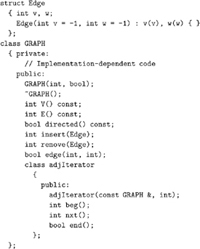
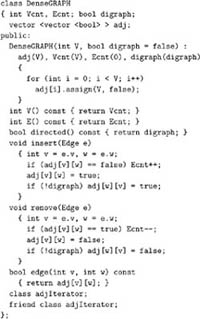
Program 17.1 Graph ADT interface
This interface is a starting point for implementing and testing graph algorithms. It defines two data types: a trivial Edge data type, including a constructor function that creates an Edge from two given vertices; and a GRAPH data type, which is defined with the standard representation-independent ADT interface methodology from Chapter 4.
The GRAPH constructor takes two arguments: an integer giving the number of vertices and a boolean that tells whether the graph is undirected or directed (a digraph), with undirected the default.
The basic operations that we use to process graphs and digraphs are ADT functions to create and destroy them; to report the number of vertices and edges; and to add and delete edges. The iterator class adjIterator allows clients to process each of the vertices adjacent to any given vertex. Programs 17.2 and 17.3 illustrate its use.
graphs (by removing some edges and adding others), and to examine the graphs (using an iterator for processing the vertices adjacent to any given vertex).
The ADT in Program 17.1 is primarily a vehicle to allow us to develop and test algorithms; it is not a general-purpose interface. As usual, we work with the simplest interface that supports the basic graph-processing operations that we wish to consider. Defining such an interface for use in practical applications involves making numerous tradeoffs among simplicity, efficiency, and generality. We consider a few of these tradeoffs next; we address many others in the context of implementations and applications throughout this book.
The graph constructor takes the maximum possible number of vertices in the graph as an argument, so that implementations can allocate memory accordingly. We adopt this convention solely to make the code compact and readable. A more general graph ADT might include in its interface the capability to add and remove vertices as well as edges; this would impose more demanding requirements on the data structures used to implement the ADT. We might also choose to work at an intermediate level of abstraction, and consider the design of interfaces that support higher-level abstract operations on graphs that we can use in implementations. We revisit this idea briefly in Section 17.5, after we consider several concrete representations and implementations.
A general graph ADT needs to take into account parallel edges and self-loops, because nothing prevents a client program from calling insert with an edge that is already present in the graph (parallel edge) or with an edge whose two vertex indices are the same (self-loop). It might be necessary to disallow such edges in some applications, desirable to include them in other applications, and possible to ignore them in still other applications. Self-loops are trivial to handle, but parallel edges can be costly to handle, depending on the graph representation. In certain situations, including a remove parallel edges ADT function might be appropriate; then, implementations can let parallel edges collect, and clients can remove or otherwise process parallel edges when warranted. We will revisit these issues when we examine graph representations in Sections 17.3 and 17.4.
Program 17.2 is a function that illustrates the use of the iterator class in the graph ADT. It is a function that extracts a graph’s
set of edges and returns it in a C++ Standard Template Library (STL) vector. A graph is nothing more nor less than its set of edges, and we often need a way to retrieve a graph in this form, regardless of its internal representation. The order in which the edges appear in the vector is immaterial and will differ from implementation to implementation. We use a template for such functions to allow for using multiple implementations of the graph ADT.
Program 17.3 is another example of the use of the iterator class in the graph ADT, to print out a table of the vertices adjacent to each vertex, as shown in Figure 17.7. The code in these two examples is quite similar and is similar to the code in numerous graph-processing algorithms. Remarkably, we can build all of the algorithms that we consider in this book on this basic abstraction of processing all the vertices adjacent to each vertex (which is equivalent to processing all the edges in the graph), as in these functions.
Figure 17.7 Adjacency lists format
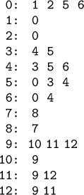
This table illustrates yet another way to represent the graph in Figure 17.1: we associate each vertex with its set of adjacent vertices (those connected to it by a single edge). Each edge affects two sets: for every edge u-v in the graph, u appears in v’s set and v appears in u’s set.
As discussed in Section 17.5, we often package related graph-processing functions into a single class. Program 17.4 is an interface for such a class. It defines the show function of Program 17.3 and two functions for inserting into a graph edges taken from standard input (see Exercise 17.12 and Program 17.14 for implementations of these functions).
Generally, the graph-processing tasks that we consider in this book fall into one of three broad categories:
• Compute the value of some measure of the graph.
• Compute some subset of the edges of the graph.
• Answer queries about some property of the graph.
Examples of the first are the number of connected components and the length of the shortest path between two given vertices in the graph; examples of the second are a spanning tree and the longest cycle containing a given vertex; examples of the third are whether two given vertices are in the same connected component. Indeed, the terms that we defined in Section 17.1 immediately bring to mind a host of computational problems.
Our convention for addressing such tasks will be to build ADTs that are clients of the basic ADT in Program 17.1, but that, in turn, allow us to separate client programs that need to solve the problem from implementations. For example, Program 17.5 is an interface for a graph-connectivity ADT. We can write client programs that use this ADT to create objects that can provide the number of connected components in the graph and that can test whether or not any two vertices are in the same connected component. We describe implementations of this ADT and their performance characteristics in Section 18.5, and we develop similar ADTs throughout the book. Typically, such ADTs include a preprocessing public member function (usually the constructor), private data members that keep information learned during the preprocessing, and query public member functions that use this information to provide clients with information about the graph.
In this book, we generally work with static graphs, which have a fixed number of vertices V and edges E. Generally, we build the graphs by executing E calls to insert, then process them either by calling some ADT function that takes a graph as argument and returns some information about that graph, or by using objects of the kind just described to preprocess the graph so as to be able to efficiently answer queries about it. In either case, changing the graph by calling insert or remove necessitates reprocessing the graph. Dynamic problems,
where we want to intermix graph processing with edge and vertex insertion and removal, take us into the realm of online algorithms (also known as dynamic algorithms ), which present a different set of challenges. For example, the connectivity problem that we solved with union-find algorithms in Chapter 1 is an example of an online algorithm, because we can get information about the connectivity of a graph as we insert edges. The ADT in Program 17.1 supports insert edge and remove edge operations, so clients are free to use them to make changes in graphs, but there may be performance penalties for certain sequences of operations. For example, union-find algorithms may require reprocessing the whole graph if a client uses remove edge. For most of the graph-processing problems that we consider, adding or deleting a few edges can dramatically change the nature of the graph and thus necessitate reprocessing it.
One of our most important challenges in graph processing is to have a clear understanding of performance characteristics of implementations and to make sure that client programs make appropriate use of them. As with the simpler problems that we considered in
Parts 1 through 4, our use of ADTs makes it possible to address such issues in a coherent manner.
Program 17.6 is an example of a graph-processing client program. It uses the basic ADT of Program 17.1, the input-output class of Program 17.4 to read the graph from standard input and print it to standard output, and the connectivity class of Program 17.5 to find its number of connected components. We use similar but more sophisticated clients to generate other types of graphs, to test algorithms, to learn other properties of graphs, and to use graphs to solve other problems. The basic scheme is amenable for use in any graph-processing application.
In Sections 17.3 through 17.5, we examine the primary classical graph representations and implementations of the ADT functions in Program 17.1. These implementations provide a basis for us to expand the interface to include the graph-processing tasks that are our focus for the next several chapters.
The first decision that we face in developing an ADT implementation is which graph representation to use. We have three basic requirements. First, we must be able to accommodate the types of graphs that we are likely to encounter in applications (and we also would prefer not to waste space). Second, we should be able to construct the requisite data structures efficiently. Third, we want to develop efficient algorithms to solve our graph-processing problems without being unduly hampered by any restrictions imposed by the representation. Such requirements are standard ones for any domain that we consider—we emphasize them again them here because, as we shall see, different representations give rise to huge performance differences for even the simplest of problems.
For example, we might consider a vector of edges representation as the basis for an ADT implementation (see Exercise 17.16). That direct representation is simple, but it does not allow us to perform efficiently the basic graph-processing operations that we shall be studying. As we will see, most graph-processing applications can be handled reasonably with one of two straightforward classical representations that are only slightly more complicated than the vector-of-edges representation: the adjacency-matrix or the adjacency-lists representation. These representations, which we consider in detail in Sections 17.3 and 17.4, are based on elementary data structures (indeed, we discussed them both in Chapters 3 and 5 as example applications of sequential and linked allocation). The choice between the two depends primarily on whether the graph is dense or sparse, although, as usual, the nature of the operations to be performed also plays an important role in the decision on which to use.
Exercises
• 17.12 Implement the scanEZ function from Program 17.4: write a function that builds a graph by reading edges (pairs of integers between 0 and V− 1) from standard input.
• 17.13 Write an ADT client that adds all the edges in a given vector to a given graph.
• 17.14 Write a function that calls edges and prints out all the edges in the graph, in the format used in this text (vertex numbers separated by a hyphen).
• 17.15 Develop an implementation for the connectivity ADT of Program 17.5, using a union-find algorithm (see Chapter 1).
• 17.16 Provide an implementation of the ADT functions in Program 17.1 that uses a vector of edges to represent the graph. Use a brute-force implementation of remove that removes an edge v-w by scanning the vector to find v-w or w-v and then exchanges the edge found with the final one in the vector. Use a similar scan to implement the iterator. Note: Reading Section 17.3 first might make this exercise easier.
17.3 Adjacency-Matrix Representation
An adjacency-matrix representation of a graph is a V -by-V matrix of Boolean values, with the entry in row v and column w defined to be 1 if there is an edge connecting vertex v and vertex w in the graph, and to be 0 otherwise. Figure 17.8 depicts an example.
Program 17.7 is an implementation of the graph ADT interface that uses a direct representation of this matrix, built as a vector of vectors, as depicted in Figure 17.9. It is a two-dimensional existence table with the entry adj[v][w] set to true if there is an edge connecting v and w in the graph, and set to false otherwise. Note that maintaining this property in an undirected graph requires that each edge be represented by two entries: the edge v-w is represented by true values in both adj[v][w] and adj[w][v], as is the edge w-v.
The name DenseGRAPH in Program 17.7 emphasizes that the implementation is more suited for dense graphs than for sparse ones, and distinguishes it from other implementations. Clients may use typedef to make this type equivalent to GRAPH or use DenseGRAPH explicitly.
In the adjacency matrix that represents a graph G, row v is a vector that is an existence table whose ith entry is true if vertex i is adjacent to v (the edge v-i is in G). Thus, to provide clients with the capability to process the vertices adjacent to v, we need only provide code that scans through this vector to find true entries, as shown in Program 17.8. We need to be mindful that, with this implementation, processing all of the vertices adjacent to a given vertex requires (at least) time proportional to V, no matter how many such vertices exist.
As mentioned in Section 17.2, our interface requires that the number of vertices is known to the client when the graph is initialized. If desired, we could allow for inserting and deleting vertices (see Exercise 17.21). A key feature of the constructor in Program 17.7 is
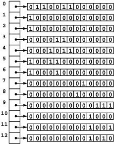
Figure 17.8 Adjacency-matrix graph representation
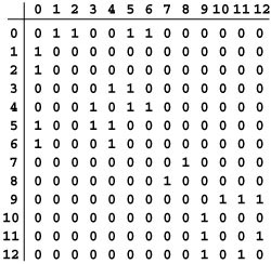
This Boolean matrix is another representation of the graph depicted in Figure 17.1. It has a 1 (true) in row v and column w if there is an edge connecting vertex v and vertex w and a 0 (false) in row v and column w if there is no such edge. The matrix is symmetric about the diagonal. For example, the sixth row (and the sixth column) says that vertex 6 is connected to vertices 0 and 4. For some applications, we will adopt the convention that each vertex is connected to itself, and assign 1s on the main diagonal. The large blocks of 0s in the upper right and lower left corners are artifacts of the way we assigned vertex numbers for this example, not characteristic of the graph (except that they do indicate the graph to be sparse).
Program 17.7 Graph ADT implementation (adjacency matrix)
This class is a straightforward implementation of the interface in Program 17.1 that is based on representing the graph with a vector of boolean vectors (see Figure 17.9). Edges are inserted and removed in constant time. Duplicate edge insert requests are silently ignored, but clients can use edge to test whether an edge exists. Constructing the graph takes time proportional to V2.
that it initializes the graph by setting the matrix entries all to false. We need to be mindful that this operation takes time proportional to V2, no matter how many edges are in the graph. Error checks for insufficient memory are not included in Program 17.7 for brevity—it is prudent programming practice to add them before using this code (see Exercise 17.24).
To add an edge, we set the indicated matrix entries to true (one for digraphs, two for undirected graphs). This representation does not allow parallel edges: If an edge is to be inserted for which the matrix entries are already 1, the code has no effect. In some ADT designs, it might be preferable to inform the client of the attempt to insert a parallel edge, perhaps using a return code from insert. This representation does allow self-loops: An edge v-v is represented by a nonzero entry in a[v][v].
Figure 17.9 Adjacency matrix data structure
This figure depicts the C++ representation of the graph in Figure 17.1, as an vector of vectors.
To remove an edge, we set the indicated matrix entries to false. If a nonexistent edge (one for which the matrix entries are already false) is to be removed, the code has no effect. Again, in some ADT designs, we might wish to arrange to inform the client of such conditions.
If we are processing huge graphs or huge numbers of small graphs, or space is otherwise tight, there are several ways to save space. For example, adjacency matrices that represent undirected graphs are symmetric: a[v][w] is always equal to a[w][v]. Thus, we could save space by storing only one-half of this symmetric matrix (see Exercise 17.22). Another way to save a signigicant amount of space is to use a matrix of bits (assuming that vector<bool> does not do so). In this way, for instance, we could represent graphs of up to about 64,000 vertices in about 64 million 64-bit words (see Exercise 17.23). These implementations have the slight complication that we need to add an ADT operation to test for the existence of an edge (see Exercise 17.20). (We do not use such an operation in our implementations because we can test for the existence of an edge v-w by simply testing a[v][w].) Such space-saving techniques are effective, but come at the cost of extra overhead that may fall in the inner loop in time-critical applications.
Many applications involve associating other information with each edge—in such cases, we can generalize the adjacency matrix to hold any information whatever, not just bools. Whatever data type that we use for the matrix elements, we need to include an indication whether the indicated edge is present or absent. In Chapters 20 and 21, we explore such representations.
Use of adjacency matrices depends on associating vertex names with integers between 0 and V − 1. This assignment might be done in one of many ways—for example, we consider a program that does so in Section 17.6). Therefore, the specific matrix of 0-1 values that we represent with a vector of vectors in C++ is but one possible representation of any given graph as an adjacency matrix, because another program might assign different vertex names to the indices we use to specify rows and columns. Two matrices that appear to be markedly different could represent the same graph (see Exercise 17.17). This observation is a restatement of the graph isomorphism problem: Although we might like to determine whether or not two different matrices represent the same graph, no one has devised an algorithm that can always do so efficiently. This difficulty is fundamental. For example, our ability to find an efficient solution to various important graph-processing problems depends completely on the way in which the vertices are numbered (see, for example, Exercise 17.26).
Program 17.3, which we considered in Section 17.2, prints out a table with the vertices adjacent to each vertex. When used with the implementation in Program 17.7, it prints the vertices in order of their vertex index, as in Figure 17.7. Notice, though, that it is not part of the definition of adjIterator that it visits vertices in index order, so developing an ADT client that prints out the adjacency-matrix representation of a graph is not a trivial task (see Exercise 17.18). The output produced by these programs are themselves graph representations that clearly illustrate a basic performance tradeoff. To print out the matrix, we need room on the page for all V2 entries; to print out the lists, we need room for just V + E numbers. For sparse graphs, when V2 is huge compared to V + E, we prefer the lists; for dense graphs, when E and V2 are comparable, we prefer the matrix. As we shall soon see, we make the same basic tradeoff when we compare the adjacency-matrix representation with its primary alternative: an explicit representation of the lists.
The adjacency-matrix representation is not satisfactory for huge sparse graphs: We need at least V2 bits of storage and V2 steps just to construct the representation. In a dense graph, when the number of edges (the number of 1 bits in the matrix) is proportional to V2, this cost may be acceptable, because time proportional to V2 is required to process the edges no matter what representation we use. In a sparse graph, however, just initializing the matrix could be the dominant factor in the running time of an algorithm. Moreover, we may not even have enough space for the matrix. For example, we may be faced with graphs with millions of vertices and tens of millions of edges, but we may not want—or be able—to pay the price of reserving space for trillions of 0 entries in the adjacency matrix.
On the other hand, when we do need to process a huge dense graph, then the 0-entries that represent absent edges increase our space needs by only a constant factor and provide us with the ability to determine whether any particular edge is present in constant time. For example, disallowing parallel edges is automatic in an adjacency matrix but is costly in some other representations. If we do have space available to hold an adjacency matrix, and either V2 is so small as to represent a negligible amount of time or we will be running a complex algorithm that requires more than V2 steps to complete, the adjacency-matrix representation may be the method of choice, no matter how dense the graph.
Exercises
• 17.17 Give the adjacency-matrix representations of the three graphs depicted in Figure 17.2.
• 17.18 Give an implementation of show for the representation-independent io package of Program 17.4 that prints out a two-dimensional matrix of 0s and 1s like the one illustrated in Figure 17.8. Note: You cannot depend upon the iterator producing vertices in order of their indices.
17.19 Given a graph, consider another graph that is identical to the first, except that the names of (integers corresponding to) two vertices are interchanged. How are the adjacency matrices of these two graphs related?
• 17.20 Add a function edge to the graph ADT that allows clients to test whether there is an edge connecting two given vertices, and provide an implementation for the adjacency-matrix representation.
• 17.21 Add functions to the graph ADT that allow clients to insert and delete vertices, and provide implementations for the adjacency-matrix representation.
• 17.22 Modify Program 17.7, augmented as described in Exercise 17.20, to cut its space requirements about in half by not including array entries a[v][w] for w greater than v.
17.23 Modify Program 17.7, augmented as described in Exercise 17.20, to ensure that, if your computer has B bits per word, a graph with V vertices is represented in about V2/B words (as opposed to V2). Do empirical tests to assess the effect of packing bits into words on the time required for the ADT operations.
17.24 Describe what happens if there is insufficient memory available to represent the matrix when the constructor in Program 17.7 is invoked, and suggest appropriate modifications to the code to handle this situation.
17.25 Develop a version of Program 17.7 that uses a single vector with V2 entries.
• 17.26 Suppose that all k vertices in a group have consecutive indices. How can you determine from the adjacency matrix whether or not that group of vertices constitutes a clique? Write a client ADT function that finds, in time proportional to V2, the largest group of vertices with consecutive indices that constitutes a clique.
17.4 Adjacency-Lists Representation
The standard representation that is preferred for graphs that are not dense is called the adjacency-lists representation, where we keep track of all the vertices connected to each vertex on a linked list that is associated with that vertex. We maintain a vector of lists so that, given a vertex, we can immediately access its list; we use linked lists so that we can add new edges in constant time.
Program 17.9 is an implementation of the ADT interface in Program 17.1 that is based on this approach, and Figure 17.10 depicts an example. To add an edge connecting v and w to this representation of the graph, we add w to v’s adjacency list and v to w’s adjacency list. In this way, we still can add new edges in constant time, but the total amount of space that we use is proportional to the number of vertices plus the number of edges (as opposed to the number of vertices squared, for the adjacency-matrix representation). For undirected graphs, we again represent each edge in two different places: an edge connecting v and w is represented as nodes on both adjacency lists. It is important to include both; otherwise, we could not answer efficiently simple questions such as, “Which vertices are adjacent to vertex v?” Program 17.10 implements the iterator that answers this question for clients, in time proportional to the number of such vertices.
The implementation in Programs 17.9 and 17.10 is a low-level one. An alternative is to use the STL list to implement each linked list (see Exercise 17.30). The disadvantage of doing so is that STL list implementations need to support many more operations than we need and therefore typically carry extra overhead that might affect the performance of all of our algorithms (see Exercise 17.31). Indeed, all of our graph algorithms use the Graph ADT interface, so this implementation is an appropriate place to encapuslate all the low-level operations and concentrate on efficiency without affecting our other code. Another advantage of using the linked-list representation is that it provides a concrete basis for understanding the performance characteristics of our implementations.
But an important factor to consider is that the linked-list–based implementation in Programs 17.9 and 17.10 is incomplete, because it lacks a destructor and a copy constructor. For many applications, this defect could lead to unexpected results or severe performance problems.
Figure 17.10 Adjacency-lists data structure
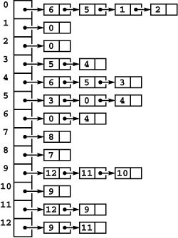
This figure depicts a representation of the graph in Figure 17.1 as an array of linked lists. The space used is proportional to the number of nodes plus the number of edges. To find the indices of the vertices connected to a given vertex v, we look at the v th position in an array, which contains a pointer to a linked list containing one node for each vertex connected to v. The order in which the nodes appear on the lists depends on the method that we use to construct the lists.
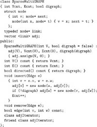
Program 17.9 Graph ADT implementation (adjacency lists)
This implementation of the interface in Program 17.1 uses a vector of linked lists, one corresponding to each vertex. It is equivalent to the representation of Program 3.15, where an edge v-w is represented by a node for w on list v and a node for v on list w.
Implementations of remove and edge are left for exercises, as are the copy constructor and the destructor. The insert code keeps insertion time constant by not checking for duplicate edges, and the total amount of space used is proportional to V + E; hence, this representation is most suitable for sparse multigraphs.
Clients may use typedef to make this type equivalent to GRAPH or use SparseMultiGRAPH explicitly.
These functions are direct extensions of those in the first-class queue implementation of Program 4.22 (see Exercise 17.29). We assume throughout the book that SparseMultiGRAPH objects have them. Using the STL list instead of low-level singly-linked lists has the distinct advantage that this extra code is unnecessary because a proper destructor and copy constructor are automatically defined. For example, DenseGRAPH objects built by Program 17.7 are properly destroyed and copied in client programs that manipulate them, because they are built from STL objects.
By contrast to Program 17.7, Program 17.9 builds multigraphs, because it does not remove parallel edges. Checking for duplicate edges in the adjacency-lists structure would necessitate searching through the lists and could take time proportional to V. Similarly, Program 17.9 does not include an implementation of the remove edge operation or the edge existence test. Adding implementations for these functions is an easy exercise (see Exercise 17.28), but each operation might take time proportional to V, to search through the lists for the nodes that represent the edges. These costs make the basic adjacency-lists representation unsuitable for applications involving huge graphs where parallel edges cannot be tolerated, or applications involving heavy use of remove edge or of edge existence tests. In Section 17.5, we discuss adjacency-list implementations that support constant-time remove edge and edge existence operations.
When a graph’s vertex names are not integers, then (as with adjacency matrices) two different programs might associate vertex names with the integers from 0 to V − 1 in two different ways, leading to two different adjacency-list structures (see, for example, Program 17.15). We cannot expect to be able to tell whether two different structures represent the same graph because of the difficulty of the graph isomorphism problem.
Moreover, with adjacency lists, there are numerous representations of a given graph even for a given vertex numbering. No matter in what order the edges appear on the adjacency lists, the adjacency-list structure represents the same graph (see Exercise 17.33). This characteristic of adjacency lists is important to know because the order in which edges appear on the adjacency lists affects, in turn, the order in which edges are processed by algorithms. That is, the adjacency-list structure determines how our various algorithms see the graph. Although an algorithm should produce a correct answer no matter how the edges are ordered on the adjacency lists, it might get to that answer by different sequences of computations for different orderings. If an algorithm does not need to examine all the graph’s edges, this effect might affect the time that it takes. And, if there is more than one correct answer, different input orderings might lead to different output results.
The primary advantage of the adjacency-lists representation over the adjacency-matrix representation is that it always uses space proportional to E + V, as opposed to V2 in the adjacency matrix. The primary disadvantage is that testing for the existence of specific edges can take time proportional to V, as opposed to constant time in the adjacency matrix. These differences trace, essentially, to the difference between using linked lists and vectors to represent the set of vertices incident on each vertex.
Thus, we see again that an understanding of the basic properties of linked data structures and vectors is critical if we are to develop efficient graph ADT implementations. Our interest in these performance differences is that we want to avoid implementations that are inappropriately inefficient under unexpected circumstances when a wide range of operations is to be demanded of the ADT. In Section 17.5, we discuss the application of basic data structures to realize many of the theoretical benefits of both structures. Nonetheless, Program 17.9 is a simple implementation with the essential characteristics that we need to learn efficient algorithms for processing sparse graphs.
Exercises
• 17.27 Show, in the style of Figure 17.10, the adjacency-lists structure produced when you use Program 17.9 to insert the edges in the graph
3-7 1-4 7-8 0-5 5-2 3-8 2-9 0-6 4-9 2-6 6-4
(in that order) into an initially empty graph.
17.28 Provide implementations of remove and edge for the adjacency-lists graph class (Program 17.9 ). Note: Duplicates may be present, but it suffices to remove any edge connecting the specified vertices.
17.29 Add a copy constructor and a destructor to the adjacency-lists graph class (Program 17.9 ). Hint: See Program 4.22.
• 17.30 Modify the implementation of SparseMultiGRAPH Programs 17.9 and 17.10 to use an STL list instead of a linked list for each adjacency list.
17.31 Run empirical tests to compare your SparseMultiGRAPH implementation of Exercise 17.30 with the implementation in the text. For a well-chosen set of values for V, compare running times for a client program that builds complete graphs with V vertices, then extracts the edges using Program 17.2.
• 17.32 Give a simple example of an adjacency-lists graph representation that could not have been built by repeated insertion of edges by Program 17.9.
17.33 How many different adjacency-lists representations represent the same graph as the one depicted in Figure 17.10?
• 17.34 Add a public member function declaration to the graph ADT (Pro-gram 17.1) that removes self-loops and parallel edges. Provide the trivial implementation of this function for the adjacency-matrix–based class (Pro-gram 17.7), and provide an implementation of the function for the adjacency-list–based class (Program 17.9) that uses time proportional to E and extra space proportional to V.
17.35 Write a version of Program 17.9 that disallows parallel edges (by scanning through the adjacency list to avoid adding a duplicate entry on each edge insertion) and self-loops. Compare your implementation with the implementation described in Exercise 17.34. Which is better for static graphs?Note: See Exercise 17.49 for an efficient implementation.
17.36 Write a client of the graph ADT that returns the result of removing self-loops, parallel edges, and degree-0 (isolated) vertices from a given graph. Note: The running time of your program should be linear in the size of the graph representation.
• 17.37 Write a client of the graph ADT that returns the result of removing self-loops, collapsing paths that consist solely of degree-2 vertices from a given graph. Specifically, every degree-2 vertex in a graph with no parallel edges appears on some path u-…-w where u and w are either equal or not of degree 2. Replace any such path with u-w, and then remove all unused degree-2 vertices as in Exercise 17.36. Note: This operation may introduce self-loops and parallel edges, but it preserves the degrees of vertices that are not removed.
• 17.38 Give a (multi)graph that could result from applying the transformation described in Exercise 17.37 on the sample graph in Figure 17.1.
17.5 Variations, Extensions, and Costs
In this section, we describe a number of options for improving the graph representations discussed in Sections 17.3 and 17.4. The topics fall into one of three categories. First, the basic adjacency-matrix and adjacency-lists mechanisms extend readily to allow us to represent other types of graphs. In the relevant chapters, we consider these extensions in detail and give examples; here, we look at them briefly. Second, we discuss graph ADT designs with more features than our basic one and implementations that use more advanced data structures to efficiently implement them. Third, we discuss our general approach to addressing graph-processing tasks, by developing task-specific classes that use the basic graph ADT.
Our implementations in Programs 17.7 and 17.9 build digraphs if the call to the constructor includes a second argument with value true. We represent each edge just once, as illustrated in Figure 17.11. An edge v-w in a digraph is represented by a 1 in the entry in row v and column w in the adjacency matrix or by the appearance of w on v’s adjacency list in the adjacency-lists representation. These representations are simpler than the corresponding representations that we have been considering for undirected graphs, but the asymmetry makes digraphs more complicated combinatorial objects than undirected graphs, as we see in Chapter 19. For example, the standard adjacency-lists representation gives no direct way to find all edges coming into a vertex in a digraph, so we would need to choose a different representation if that operation needs to be supported.
Figure 17.11 Digraph representations
The adjacency-matrix and adjacency-lists representations of a digraph have only one representation of each edge, as illustrated in the adjacency-matrix (top) and adjacency-lists (bottom) representation of the set of edges in Figure 17.1 interpreted as a digraph (see Figure 17.6, top).
For weighted graphs and networks, we fill the adjacency matrix with structures containing information about edges (including their presence or absence) instead of Boolean values; in the adjacency-lists representation, we include this information in adjacency-list elements.
It is often necessary to associate still more information with the vertices or edges of a graph, to allow that graph to model more complicated objects. We can associate extra information with each edge by extending the Edge type in Program 17.1 as appropriate, then using instances of that type in the adjacency matrix, or in the list nodes in the adjacency lists. Or, since vertex names are integers between 0 and V − 1, we can use vertex-indexed vectors to associate extra information for vertices, perhaps using an appropriate ADT. We consider ADTs of this sort in Chapters 20 through 22. Alternatively, we could use a separate symbol-table ADT to associate extra information with each vertex and edge (see Exercise 17.48 and Program 17.15).
To handle various specialized graph-processing problems, we often define classes that contain specialized auxiliary data structures related to the graph. The most common such data structure is a vertex-indexed vector, as we saw already in Chapter 1, where we used vertex-indexed vectors to answer connectivity queries. We use vertex-indexed vectors in numerous implementations throughout the book.
As an example, suppose that we wish to know whether a vertex v in a graph is isolated. Is v of degree 0? For the adjacency-lists representation, we can find this information immediately, simply by checking whether adj[v] is null. But for the adjacency-matrix representation, we need to check all V entries in the row or column corresponding to v to know that each one is not connected to any other vertex; and for the vector-of-edges representation, we have no better approach than to check all E edges to see whether there are any that involve v. We need to enable clients to avoid these potentially time-consuming computations. As discussed in Section 17.2 one way to do so is to define a client ADT for the problem, such as the example in Program 17.11. This implementation, after preprocessing the graph in time proportional to the size of its representation, allows clients to find the degree of any
vertex in constant time. That is no improvement if the client needs the degree of just one vertex, but it represents a substantial savings for clients that need to know the degrees of many vertices. Such a substantial performance differential for such a simple problem is typical in graph processing.
For each of the graph-processing tasks that we consider in this book, we encapsulate solutions in classes like this one, with private data and function members and public function members specific to the task. Clients create objects whose member functions do the graph processing. This approach amounts to extending the graph ADT interface by defining a cooperating set of classes. Any set of such classes defines a graph-processing interface, but each encapsulates its own private data and function members.
There are many other ways to build upon an interface in C++. One way to proceed is to simply add public function members (and whatever private data and function members we might need) to the basic GRAPH ADT definition. While this approach has all of the virtues extolled in Chapter 4, it also has some serious drawbacks, because the world of graph-processing is significantly more expansive than the kinds of basic data structures that are the subject of Chapter 4. Chief among these drawbacks are the following:
• There are many more graph-processing functions to implement than we can accurately define in a single interface.
• Simple graph-processing tasks have to use the same interface needed by complicated tasks.
• One member function can access a data member intended for use by another member function, contrary to encapsulation principles that we would like to follow.
Interfaces of this kind have come to be known as fat interfaces. In a book filled with graph-processing algorithms, an interface of this sort would be fat indeed.
Another approach is to use inheritance to define various types of graphs that provide clients with various sets of graph-processing tasks. Comparing the intricacies of this approach with the simpler approach that we use is a worthwhile exercise in the study of software engineering, but would take us still further afield from the subject of graph-processing algorithms, our main focus.
Table 17.1 shows the dependence of the cost of various simple graph-processing operations on the representation that we use. This table is worth examining before we consider the implementation of more complicated operations; it will help you to develop an intuition for the difficulty of various primitive operations. Most of the costs listed follow immediately from inspecting the code, with the exception of the bottom row, which we consider in detail at the end of this section.
In several cases, we can modify the representation to make simple operations more efficient, although we have to take care that doing so does not increase costs for other simple operations. For example, the entry for adjacency-matrix destroy is an artifact of our vector-of-vectors
Table 17.1 Worst-case cost of graph-processing operations
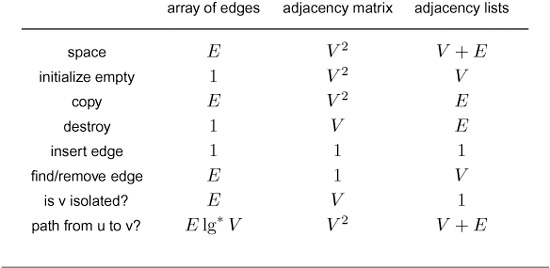
The performance characteristics of basic graph-processing ADT operations for different graph representations vary widely, even for simple tasks, as indicated in this table of the worst-case costs (all within a constant factor for large V and E ). These costs are for the simple implementations we have described in previous sections; various modifications that affect the costs are described in the text of this section.
allocation scheme for two-dimensional matrices (see Section 3.7). It is not difficult to reduce this cost to be constant (see Exercise 17.25). On the other hand, if graph edges are sufficiently complex structures that the matrix entries are pointers, then to destroy an adjacency matrix would take time proportional to V2.
Because of their frequent use in typical applications, we consider the find edge and remove edge operations in detail. In particular, we need a find edge operation to be able to remove or disallow parallel edges. As we saw in Section 17.3, these operations are trivial if we are using an adjacency-matrix representation—we need only to check or set a matrix entry that we can index directly. But how can we implement these operations efficiently in the adjacency-lists representation? In C++, we could use the STL; here we describe underlying mechanisms, to gain perspective on efficiency issues. One approach is described next, and another is described in Exercise 17.50. Both approaches are based on symbol-table implementations. If we use, for example, dynamic hash table implementations (see Section 14.5), both approaches take space proportional to E andallowustoperform either operation in constant time (on the average, amortized).
Specifically, to implement find edge when we are using adjacency lists, we could use an auxiliary symbol table for the edges. We can assign an edge v-w the integer key v*V+w and use an STL map or any of the symbol-table implementations from Part 4. (For undirected graphs, we might assign the same key to v-w and w-v.) We can insert each edge into the symbol table, after first checking whether it has already been inserted. We can choose either to disallow parallel edges (see Exercise 17.49) or to maintain duplicate records in the symbol table for parallel edges (see Exercise 17.50). In the present context, our main interest in this technique is that it provides a constant-time find edge implementation for adjacency lists.
To be able to remove edges, we need a pointer in the symbol-table record for each edge that refers to its representation in the adjacency-lists structure. But even this information is not sufficient to allow us to remove the edge in constant time unless the lists are doubly linked (see Section 3.4). Furthermore, in undirected graphs, it is not sufficient to remove the node from the adjacency list, because each edge appears on two different adjacency lists. One solution to this difficulty is to put both pointers in the symbol table; another is to link together the two list nodes that correspond to a particular edge (see Exercise 17.46). With either of these solutions, we can remove an edge in constant time.
Removing vertices is more expensive. In the adjacency-matrix representation, we essentially need to remove a row and a column from the matrix, which is not much less expensive than starting over again with a smaller matrix (although that cost can be amortized using the same mechanism as for dynamic hash tables). If we are using an adjacency-lists representation, we see immediately that it is not sufficient to remove nodes from the vertex’s adjacency list, because each node on the adjacency list specifies another vertex whose adjacency list we must search to remove the other node that represents the same edge. We need the extra links to support constant-time edge removal as described in the previous paragraph if we are to remove a vertex in time proportional to V.
We omit implementations of these operations here because they are straightforward programming exercises using basic techniques from Part 1, because the STL provides implementations that we could use, because maintaining complex structures with multiple pointers per node is not justified in typical applications that involve static graphs, and because we wish to avoid getting bogged down in layers of abstraction or in low-level details of maintaining multiple pointers when implementing graph-processing algorithms that do not otherwise use them. In Chapter 22, we do consider implementations of a similar structure that play an essential role in the powerful general algorithms that we consider in that chapter.
For clarity in describing and developing implementations of algorithms of interest, we use the simplest appropriate representation. Generally, we strive to use data structures that are directly relevant to the task at hand. Many programmers practice this kind of minimalism as a matter of course, knowing that maintaining the integrity of a data structure with multiple disparate components can be a challenging task, indeed.
We might also consider alternate implementations that modify the basic data structures in a performance-tuning process to save space or time, particularly when processing huge graphs (or huge numbers of small graphs). For example, we can dramatically improve the performance of algorithms that process huge static graphs represented with adjacency lists by stripping down the representation to use vectors of varying length instead of linked lists to represent the set of vertices incident on each vertex. With this technique, we can ultimately represent a graph with just 2E integers less than V and V integers less than V2 (see Exercises 17.52 and 17.54). Such representations are attractive for processing huge static graphs.
The algorithms that we consider adapt readily to all the variations that we have discussed in this section, because they are based on a few high-level abstract operations such as “perform the following operation for each edge adjacent to vertex v” that are supported by our basic ADT.
In some instances, our algorithm-design decisions depend on certain properties of the representation. Working at a higher level of abstraction might obscure our knowledge of that dependence. If we know that one representation would lead to poor performance but another would not, we would be taking an unnecessary risk were we to consider the algorithm at the wrong level of abstraction. As usual, our goal is to craft implementations such that we can make precise statements about performance. For this reason, though both implement the basic graph ADT, we retain separate DenseGRAPH and SparseMultiGRAPH types for the adjacency-matrix and adjacency-lists representations, respectively, to emphasize that clients can use these implementations as appropriate to suit the task at hand.
All of the operations that we have considered so far are simple, albeit necessary, data-processing functions; and the bottom line of the discussion in this section is that basic algorithms and data structures from Parts 1 through 3 are effective for handling them. As we develop more sophisticated graph-processing algorithms, we face more diffi-cult challenges in finding the best implementations for specific practical problems. To illustrate this point, we consider the last row in Table 17.1, which gives the costs of determining whether there is a path connecting two given vertices.
In the worst case, the simple path-finding algorithm in Section 17.7 examines all E edges in the graph (as do several other methods that we consider in Chapter 18). The entries in the center and right column on the bottom row in Table 17.1 indicate, respectively, that the algorithm may examine all V2 entries in an adjacency-matrix representation, and all V list heads and all E nodes on the lists in an adjacency-lists representation. These facts imply that the algorithm’s running time is linear in the size of the graph representation, but they also exhibit two anomalies: The worst-case running time is not linear in the number of edges in the graph if we are using an adjacency-matrix representation for a sparse graph or either representation for an extremely sparse graph (one with a huge number of isolated vertices). To avoid repeatedly considering these anomalies, we assume throughout that the size of the representation that we use is proportional to the number of edges in the graph. This point is moot in the majority of applications because they involve huge sparse graphs and thus require an adjacency-lists representation.
The left column on the bottom row in Table 17.1 derives from the use of the union-find algorithms in Chapter 1 (see Exercise 17.15). This method is attractive because it only requires space proportional to V, but has the drawback that it cannot exhibit the path. This entry highlights the importance of completely and precisely specifying graph-processing problems.
Even after taking all of these factors into consideration, one of the most significant challenges that we face when developing practical graph-processing algorithms is assessing the extent to which the results of worst-case performance analyses, such as those in Table 17.1, over-estimate time and space needs for processing graphs that we encounter in practice. Most of the literature on graph algorithms describes performance in terms of such worst-case guarantees, and, while this information is helpful in identifying algorithms that can have unacceptably poor performance, it may not shed much light on which of several simple, direct programs may be most suitable for a given application. This situation is exacerbated by the difficulty of developing useful models of average-case performance for graph algorithms, leaving us with (perhaps unreliable) benchmark testing and (perhaps overly conservative) worst-case performance guarantees to work with. For example, the graph-search methods that we discuss in Chapter 18 are all effective linear-time algorithms for finding a path between two given vertices, but their performance characteristics differ markedly, depending both upon the graph being processed and its representation. When using graph-processing algorithms in practice, we constantly fight this disparity between the worst-case performance guarantees that we can prove and the actual performance characteristics that we can expect. This theme will recur throughout the book.
Exercises
• 17.39 Develop an adjacency-matrix representation for dense multigraphs, and provide an ADT implementation for Program 17.1 that uses it.
• 17.40 Why not use a direct representation for graphs (a data structure that models the graph exactly, with vertex objects that contain adjacency lists with references to the vertices)?
• 17.41 Why does Program 17.11 not increment both deg[v] and deg[w] when it discovers that w is adjacent to v?
• 17.42 Add to the graph class that uses adjacency matrices (Program 17.7) a vertex-indexed vector that holds the degree of each vertex. Add a public member function degree that returns the degree of a given vertex.
17.43 Do Exercise 17.42 for the adjacency-lists representation.
• 17.44 Add a row to Table 17.1 for the problem of determining the number of isolated vertices in a graph. Support your answer with function implementations for each of the three representations.
• 17.45 Give a row to add to Table 17.1 for the problem of determining whether a given digraph has a vertex with indegree V and outdegree 0. Support your answer with function implementations for each of the three representations. Note: Your entry for the adjacency-matrix representation should be V.
17.46 Use doubly-linked adjacency lists with cross links as described in the text to implement a constant-time remove edge function remove for the graph ADT implementation that uses adjacency lists (Program 17.9).
17.47 Add a remove vertex function remove to the doubly-linked adjacency-lists graph class described in the previous exercise.
• 17.48 Modify your solution to Exercise 17.16 to use a dynamic hash table, as described in the text, such that insert edge and remove edge take constant amortized time.
17.49 Add to the graph class that uses adjacency lists (Program 17.9) a symbol table to ignore duplicate edges, so that it represents graphs instead of multigraphs. Use dynamic hashing for your symbol-table implementation so that your implementation uses space proportional to E and can insert, find, and remove edges in constant time (on the average, amortized).
17.50 Develop a multigraph class based on a vector-of-symbol-tables representation (with one symbol table for each vertex, which contains its list of adjacent edges). Use dynamic hashing for your symbol-table implementation so that your implementation uses space proportional to E and can insert, find, and remove edges in constant time (on the average, amortized).
17.51 Develop a graph ADT intended for static graphs, based upon a constructor that takes a vector of edges as an argument and uses the basic graph ADT to build a graph. (Such an implementation might be useful for performance comparisons with the implementations described in Exercises 17.52 through 17.55.)
17.52 Develop an implementation for the constructor described in Exercise 17.51 that uses a compact representation based on the following data structures:
struct node { int cnt; vector <int> edges; };
struct graph { int V; int E; vector <node> adj; };
A graph is a vertex count, an edge count, and a vector of vertices. A vertex contains an edge count and a vector with one vertex index corresponding to each adjacent edge.
• 17.53 Add to your solution to Exercise 17.52 a function that eliminates self-loops and parallel edges, as in Exercise 17.34.
• 17.54 Develop an implementation for the static-graph ADT described in Exercise 17.51 that uses just two vectors to represent the graph: one vector of E vertices, and another of V indices or pointers into the first vector. Implement io::show for this representation.
• 17.55 Add to your solution to Exercise 17.54 a function that eliminates self-loops and parallel edges, as in Exercise 17.34.
17.56 Develop a graph ADT interface that associates (x, y) coordinates with each vertex, so that you can work with graph drawings. Include functions drawV and drawE to draw a vertex and to draw an edge, respectively.
17.57 Write a client program that uses your interface from Exercise 17.56 to produce drawings of edges that are being added to a small graph.
17.58 Develop an implementation of your interface from Exercise 17.56 that produces a PostScript program with drawings as output (see Section 4.3).
17.59 Find an appropriate graphics interface that allows you to develop an implementation of your interface from Exercise 17.56 that directly draws graphs in a window on your display.
• 17.60 Extend your solution to Exercises 17.56 and 17.59 to include functions to erase vertices and edges and to draw them in different styles, so that you can write client programs that provide dynamic graphical animations of graph algorithms in operation.
17.6 Graph Generators
To develop further appreciation for the diverse nature of graphs as combinatorial structures, we now consider detailed examples of the types of graphs that we use later to test the algorithms that we study. Some of these examples are drawn from applications. Others are drawn from mathematical models that are intended both to have properties that we might find in real graphs and to expand the range of input trials available for testing our algorithms.
To make the examples concrete, we present them as client functions of Program 17.1, so that we can put them to immediate use when we test implementations of the graph algorithms that we consider. In addition, we consider the implementation of io::scan from Program 17.4, which reads a sequence of pairs of arbitrary names from standard input and builds a graph with vertices corresponding to the names and edges corresponding to the pairs.
The implementations that we consider in this section are based upon the interface of Program 17.1, so they function properly, in theory, for any graph representation. In practice, however, some combinations of interface and representation can have unacceptably poor performance, as we shall see.
As usual, we are interested in having “random problem instances,” both to exercise our programs with arbitrary inputs and to get an idea of how the programs might perform in real applications. For graphs, the latter goal is more elusive than for other domains that we have considered, although it is still a worthwhile objective. We shall encounter various different models of randomness, starting with these two.
Random edges This model is simple to implement, as indicated by the generator given in Program 17.12. For a given number of vertices V, we generate random edges by generating pairs of numbers between 0 and V − 1. The result is likely to be a random multigraph with self-loops. A given pair could have two identical numbers (hence, self-loops could occur); and any pair could be repeated multiple times (hence, parallel edges could occur). Program 17.12 generates edges until the graph is known to have E edges, leaving to the implementation the decision of whether to eliminate parallel edges. If parallel edges are eliminated, the number of edges generated is substantially higher than then number of edges used (E) for dense graphs (see Exercise 17.62); so this method is normally used for sparse graphs.
Figure 17.12 Two random graphs
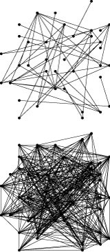
Both of these random graphs have 50 vertices. The sparse graph at the top has 50 edges, while the dense graph at the bottom has 500 edges. The sparse graph is not connected, with each vertex connected only to a few others; the dense graph is certainly connected, with each vertex connected to 20 others, on the average. These diagrams also indicate the difficulty of developing algorithms that can draw arbitrary graphs (the vertices here are placed in random position).
Random graph The classic mathematical model for random graphs is to consider all possible edges and to include each in the graph with a fixed probability p. If we want the expected number of edges in the graph to be E, we can choose p = 2E/V (V − 1). Program 17.13 is a function that uses this model to generate random graphs. This model precludes duplicate edges, but the number of edges in the graph is only equal to E on the average. This implementation is well-suited for dense graphs, but not for sparse graphs, since it runs in time proportional to V (V − 1)/2 to generate just E =pV (V - 1)/2 edges. That is, for sparse graphs, the running time of Program 17.13 is quadratic in the size of the graph (see Exercise 17.68).
These models are well-studied and are not difficult to implement, but they do not necessarily generate graphs with properties similar to the ones that we see in practice. In particular, graphs that model maps, circuits, schedules, transactions, networks, and other practical situations are usually not only sparse but also exhibit a locality property—edges are much more likely to connect a given vertex to vertices in a particular set than to vertices that are not in the set. We might consider many different ways of modeling locality, as illustrated in the following examples.
k-neighbor graph The graph depicted at the top in Figure 17.13 is drawn from a simple modification to a random-edges graph generator, where we randomly pick the first vertex v, then randomly pick the second from among those whose indices are within a fixed constant k of v (wrapping around from V − 1 to 0, when the vertices are arranged in a circle as depicted). Such graphs are easy to generate and certainly exhibit locality not found in random graphs.
Euclidean neighbor graph The graph depicted at the bottom in Figure 17.13 is drawn from a generator that generates V points in the plane with random coordinates between 0 and 1, and then generates edges connecting any two points within distance d of one another. If d is small, the graph is sparse; if d is large, the graph is dense (see Exercise 17.74). This graph models the types of graphs that we might expect when we process graphs from maps, circuits, or other applications where vertices are associated with geometric locations. They are easy to visualize, exhibit properties of algorithms in an intuitive manner, and exhibit many of the structural properties that we find in such applications.
One possible defect in this model is that the graphs are not likely to be connected when they are sparse; other difficulties are that the graphs are unlikely to have high-degree vertices and that they do not have any long edges. We can change the models to handle such situations, if desired, or we can consider numerous similar examples to try to model other situations (see, for example, Exercises 17.72 and 17.73).
Or, we can test our algorithms on real graphs. In many applications, there is no shortage of problem instances drawn from actual data that we can use to test our algorithms. For example, huge graphs drawn from actual geographic data are easy to find; two more examples are listed in the next two paragraphs. The advantage of working with real data instead of a random graph model is that we can see solutions to real problems as algorithms evolve. The disadvantage is that we may lose the benefit of being able to predict the performance of our algorithms through mathematical analysis. We return to this topic when we are ready to compare several algorithms for the same task, at the end of Chapter 18.
Transaction graph Figure 17.14 illustrates a tiny piece of a graph that we might find in a telephone company’s computers. It has a
Figure 17.13 Random neighbor graphs
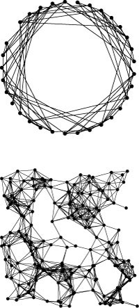
These figures illustrate two models of sparse graphs. The neighbor graph at the top has 33 vertices and 99 edges, with each edge restricted to connect vertices whose indices differ by less than 10 (modulo V ). The Euclidean neighbor graph at the bottom models the types of graphs that we might find in applications where vertices are tied to geometric locations. Vertices are random points in the plane; edges connect any pair of vertices within a specified distance d of each other. This graph is sparse (177 vertices and 1001 edges); by adjusting d, we can generate graphs of any desired density.
Figure 17.14 Transaction graph
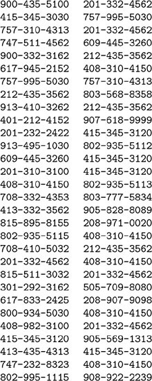
A sequence of pairs of numbers like this one might represent a list of telephone calls in a local exchange, or financial transfers between accounts, or any similar situation involving transactions between entities with unique identifiers. The graphs are hardly random—some phones are far more heavily used than others and some accounts are far more active than others.
vertex defined for each phone number, and an edge for each pair i and j with the property that i made a telephone call to j within some fixed period. This set of edges represents a huge multigraph. It is certainly sparse, since each person places calls to only a tiny fraction of the available telephones. It is representative of many other applications. For example, a financial institution’s credit card and merchant account records might have similar information.
Function call graph We can associate a graph with any computer program with functions as vertices and an edge connecting X and Y whenever function X calls function Y. We can instrument the program to create such a graph (or have a compiler do it). Two completely different graphs are of interest: the static version, where we create edges at compile time corresponding to the function calls that appear in the program text of each function; and a dynamic version, where we create edges at run time when the calls actually happen. We use static function call graphs to study program structure and dynamic ones to study program behavior. These graphs are typically huge and sparse.
In applications such as these, we face massive amounts of data, so we might prefer to study the performance of algorithms on real
Program 17.15 Symbol indexing for vertex names
This implementation of symbol-table indexing for string keys (which is described in the commentary for Program 17.14) accomplishes the task by adding an index field to each node in an existence-table TST (see Program 15.8). The index associated with each key is kept in the index field in the node corresponding to its end-of-string character.
We use the characters in the search key to move down the TST, as usual. When we reach the end of the key, we set its index if necessary and also set the private data member val, which is returned to the caller after all recursive calls to the function have returned.
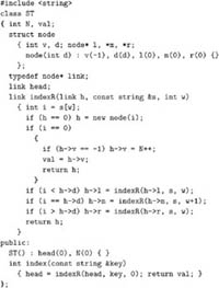
Figure 17.15 Degrees-of-separation graph
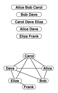
The graph at the bottom is defined by the groups at the top, with one vertex for each person and an edge connecting a pair of people whenever they are in the same group. Shortest path lengths in the graph correspond to degrees of separation. For example, Frank is three degrees of separation from Alice and Bob.
sample data rather than on random models. We might choose to try to avoid degenerate situations by randomly ordering the edges or by introducing randomness in the decision making in our algorithms, but that is a different matter from generating a random graph. Indeed, in many applications, learning the properties of the graph structure is a goal in itself.
In several of these examples, vertices are natural named objects, and edges appear as pairs of named objects. For example, a transaction graph might be built from a sequence of pairs of telephone numbers, and a Euclidean graph might be built from a sequence of pairs of cities or towns. Program 17.14 is an implementation of the scan function in Program 17.4, which we can use to build a graph in this common situation. For the client’s convenience, it takes the set of edges as defining the graph and deduces the set of vertex names from their use in edges. Specifically, the program reads a sequence of pairs of symbols from standard input, uses a symbol table to associate the vertex numbers 0 to V − 1 to the symbols (where V is the number of different symbols in the input), and builds a graph by inserting the edges, as in Programs 17.12 and 17.13. We could adapt any symbol-table implementation to support the needs of Program 17.14; Program 17.15 is an example that uses ternary search trees (TSTs) (see Chapter 14). These programs make it easy for us to test our algorithms on real graphs that may not be characterized accurately by any probabilistic model.
Program 17.14 is also significant because it validates the assumption we have made in all of our algorithms that the vertex names are integers between 0 and V − 1. If we have a graph that has some other set of vertex names, then the first step in representing the graph is to use Program 17.15 to map the vertex names to integers between 0 and V − 1.
Some graphs are based on implicit connections among items. We do not focus on such graphs, but we note their existence in the next few examples and devote a few exercises to them. When faced with processing such a graph, we can certainly write a program to construct explicit graphs by enumerating all the edges; but there also may be solutions to specific problems that do not require that we enumerate all the edges and therefore can run in sublinear time.
Degrees-of-separation graph Consider a collection of subsets drawn from V items. We define a graph with one vertex corresponding to each element in the union of the subsets and edges between two vertices if both vertices appear in some subset (see Figure 17.15). If desired, the graph might be a multigraph, with edge labels naming the appropriate subsets. All items incident on a given item v are said to be 1 degree of separation from v. Otherwise, all items incident on any item that is i degrees of separation from v (that are not already known to be i or fewer degrees of separation from v) are (i+1) degrees of separation from v. This construction has amused people ranging from mathematicians (Erdös number) to movie buffs (separation from Kevin Bacon).
Interval graph Consider a collection of V intervals on the real line (pairs of real numbers). We define a graph with one vertex corresponding to each interval, with edges between vertices if the corresponding intervals intersect (have any points in common).
de Bruijn graph Suppose that V is a power of 2. We define a digraph with one vertex corresponding to each nonnegative integer less than V, with edges from each vertex i to 2i and (2i +1) mod lg V. These graphs are useful in the study of the sequence of values that can occur in a fixed-length shift register for a sequence of operations where we repeatedly shift all the bits one position to the left, throw away the leftmost bit, and fill the rightmost bit with 0 or 1. Figure 17.16 depicts thedeBruijn graphs with 8, 16, 32, and 64 vertices.
The various types of graphs that we have considered in this section have a wide variety of different characteristics. However, they all look the same to our programs: They are simply collections of edges. As we saw in Chapter 1, learning even the simplest facts about them can be a computational challenge. In this book, we consider numerous ingenious algorithms that have been developed for solving practical problems related to many types of graphs.
Based just on the few examples presented in this section, we can see that graphs are complex combinatorial objects, far more complex than those underlying other algorithms that we studied in Parts 1 through 4. In many instances, the graphs that we need to consider in applications are difficult or impossible to characterize. Algorithms that perform well on random graphs are often of limited applicability because it is often difficult to be persuaded that random graphs have
Figure 17.16 de Bruijn graphs
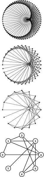
A de Bruijn digraph of order n has 2n vertices with edges from i to 2i mod n and (2i+1) mod 2n, for all i. Pictured here are the underlying undirected de Bruijn graphs of order 6, 5, 4, and 3 (top to bottom).
structural characteristics the same as those of the graphs that arise in applications. The usual approach to overcome this objection is to design algorithms that perform well in the worst case. While this approach is successful in some instances, it falls short (by being too conservative) in others.
While we are often not justified in assuming that performance studies on graphs generated from one of the random graph models that we have discussed will give information sufficiently accurate to allow us to predict performance on real graphs, the graph generators that we have considered in this section are useful in helping us to test implementations and to understand our algorithms’ performance. Before we even attempt to predict performance for applications, we must at least verify any assumptions that we might have made about the relationship between the application’s data and whatever models or sample data we may have used. While such verfication is wise when we are working in any applications domain, it is particularly important when we are processing graphs, because of the broad variety of types of graphs that we encounter.
Exercises
• 17.61 When we use Program 17.12 to generate random graphs of density αV, what fraction of edges produced are self-loops?
• 17.62 Calculate the expected number of parallel edges produced when we use Program 17.12 to generate random graphs with V vertices of density. Use the result of your calculation to draw plots showing the fraction of parallel edges produced as a function of, for V =10, 100, and 1000.
17.63 Use an STL map to develop an alternate implemention of the ST class of Program 17.15.
• 17.64 Find a large undirected graph somewhere online—perhaps based on network-connectivity information, or a separation graph defined by coauthors in a set of bibliographic lists or by actors in movies.
• 17.65 Write a program that generates sparse random graphs for a well-chosen set of values of V and E, and prints the amount of space that it used for the graph representation and the amount of time that it took to build it. Test your program with a sparse-graph class (Program 17.9) and with the random-graph generator (Program 17.12), so that you can do meaningful empirical tests on graphs drawn from this model.
• 17.66 Write a program that generates dense random graphs for a well-chosen set of values of V and E, and prints the amount of space that it used for the graph representation and the amount of time that it took to build it. Test your
program with a dense-graph class (Program 17.7) and with the random-graph generator (Program 17.13), so that you can do meaningful empirical tests on graphs drawn from this model.
• 17.67 Give the standard deviation of the number of edges produced by Program 17.13.
• 17.68 Write a program that produces each possible graph with precisely the same probability as does Program 17.13, but uses time and space proportional to only V + E, not V2. Test your program as described in Exercise 17.65.
• 17.69 Write a program that produces each possible graph with precisely the same probability as does Program 17.12, but uses time proportional to E, even when the density is close to 1. Test your program as described in Exercise 17.66.
• 17.70 Write a program that produces, with equal likelihood, each of the possible graphs with V vertices and E edges (see Exercise 17.9). Test your program as described in Exercise 17.65 (for low densities) and as described in Exercise 17.66 (for high densities).
• 17.71 Write a program that generates random graphs by connecting vertices arranged in a ![]() -by-
-by-![]() grid to their neighbors (see Figure 1.2), with k extra edges connecting each vertex to a randomly chosen destination vertex (each destination vertex equally likely). Determine how to set k such that the expected number of edges is E. Test your program as described in Exercise 17.65.
grid to their neighbors (see Figure 1.2), with k extra edges connecting each vertex to a randomly chosen destination vertex (each destination vertex equally likely). Determine how to set k such that the expected number of edges is E. Test your program as described in Exercise 17.65.
17.72 Write a program that generates random digraphs by randomly connecting vertices arranged in a ![]() -by-
-by-![]() grid to their neighbors, with each of the possible edges occurring with probability p (see Figure 1.2). Determine how to set p such that the expected number of edges is E. Test your program as described in Exercise 17.65.
grid to their neighbors, with each of the possible edges occurring with probability p (see Figure 1.2). Determine how to set p such that the expected number of edges is E. Test your program as described in Exercise 17.65.
• 17.73 Augment your program from Exercise 17.72 to add R extra random edges, computed as in Program 17.12. For large R, shrink the grid so that the total number of edges remains about V.
17.74 Write a program that generates V random points in the plane, then builds a graph consisting of edges connecting all pairs of points within a given distance d of one another (see Figure 17.13 and Program 3.20). Determine how to set d such that the expected number of edges is E. Test your program as described in Exercise 17.65 (for low densities) and as described in Exercise 17.66 (for high densities).
• 17.75 Write a program that generates V random intervals in the unit interval, all of length d, then builds the corresponding interval graph. Determine how to set d such that the expected number of edges is E. Test your program as described in Exercise 17.65 (for low densities) and as described in Exercise 17.66 (for high densities). Hint: Use a BST.
• 17.76 Write a program that chooses V vertices and E edges at random from the real graph that you found for Exercise 17.64. Test your program as described in Exercise 17.65 (for low densities) and as described in Exercise 17.66 (for high densities).
• 17.77 One way to define a transportation system is with a set of sequences of vertices, each sequence defining a path connecting the vertices. For example, the sequence 0-9-3-2 defines the edges 0-9, 9-3, and 3-2. Write a program that builds a graph from an input file consisting of one sequence per line, using symbolic names. Develop input suitable to allow you to use your program to build a graph corresponding to the Paris metro system.
17.78 Extend your solution to Exercise 17.77 to include vertex coordinates, along the lines of Exercise 17.60, so that you can work with graphical representations.
• 17.79 Apply the transformations described in Exercises 17.34 through 17.37 to various graphs (see Exercises 17.63–76), and tabulate the number of vertices and edges removed by each transformation.
• 17.80 Implement a constructor for Program 17.1 that allows clients to build separation graphs without having to call a function for each implied edge. That is, the number of function calls required for a client to build a graph should be proportional to the sum of the sizes of the groups. Develop an efficient implementation of this modified ADT (based on data structures involving groups, not implied edges).
17.81 Give a tight upper bound on the number of edges in any separation graph with N different groups of k people.
• 17.82 Draw graphs in the style of Figure 17.16 that, for V = 8, 16, and 32, have V vertices numbered from 0 to V − 1 and an edge connecting each vertex i with [floorleft]i/ 2[floorright].
17.83 Modify the ADT interface in Program 17.1 to allow clients to use symbolic vertex names and edges to be pairs of instances of a generic Vertex type. Hide the vertex-index representation and the symbol-table ADT usage completely from clients.
17.84 Add a function to the ADT interface from Exercise 17.83 that supports a join operation for graphs, and provide implementations for the adjacency-matrix and adjacency-lists representations. Note: Any vertex or edge in either graph should be in the join, but vertices that are in both graphs appear only once in the join, and you should remove parallel edges.
17.7 Simple, Euler, and Hamilton Paths
Our first nontrivial graph-processing algorithms solve fundamental problems concerning paths in graphs. They introduce the general recursive paradigm that we use throughout the book, and they illustrate
that apparently similar graph-processing problems can range widely in difficulty.
These problems take us from local properties such as the existence of edges or the degrees of vertices to global properties that tell us about a graph’s structure. The most basic such property is whether two vertices are connected. If they are, we are interested in finding a simple path that connects them.
Figure 17.17 Trace for simple path search
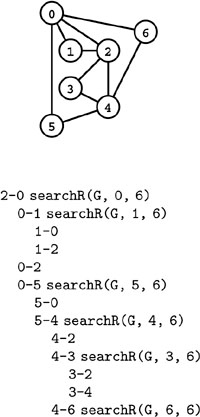
This trace shows the operation of the recursive function in Program 17.16 for the call searchR(G, 2, 6) to find a simple path from 2 to 6 in the graph shown at the top. There is a line in the trace for each edge considered, indented one level for each recursive call. To check 2-0, we call searchR(G, 0, 6). This call causes us to check 0-1, 0-2, and 0-5. To check 0-1, we call searchR(G, 1, 6), which causes us to check 1-0 and 1-2, which do not lead to recursive calls because 0 and 2 are marked. For this example, the function discovers the path 2-0-5-4-6.
Simple path Given two vertices, is there a simple path in the graph that connects them? In some applications, we might be satisfied to know merely whether or not such a path exists, but we are concerned here with the problem of finding a specific path.
Program 17.16 is a direct solution that finds a path. It is based on depth-first search, a fundamental graph-processing paradigm that we considered briefly in Chapters 3 and 5 and shall study in detail in Chapter 18. The algorithm is based on a recursive private function member that determines whether there is a simple path from v to w by checking, for each edge v-t incident on v, whether there is a simple path from t to w that does not go through v. It uses a vertex-indexed vector to mark v so that no path through v will be checked in any recursive call.
The code in Program 17.16 simply tests for the existence of a path. How can we augment it to print the path’s edges? Thinking recursively suggests an easy solution:
• Add a statement to print t-v just after the recursive call in searchR finds a path from t to w.
• Switch w and v in the call on searchR in the constructor.
Alone, the first change would cause the path from v to w to be printed in reverse order: If the call to searchR(t, w) finds a path from t to w (and prints that path’s edges in reverse order), then printing t-v completes the job for the path from v to w. The second change reverses the order: To print the edges on the path from v to w, we print the edges on the path from w to v in reverse order. (This trick only works for undirected graphs.) We could use this same strategy to implement an ADT function that calls a client-supplied function for each of the path’s edges (see Exercise 17.88).
Figure 17.17 gives an example of the dynamics of the recursion. As with any recursive program (indeed, any program with function calls at all), such a trace is easy to produce: To modify Program 17.16 to produce one, we can add a variable depth that is incremented on entry and decremented on exit to keep track of the depth of the recursion, then add code at the beginning of the recursive function to print out depth spaces followed by the appropriate information (see Exercises 17.86 and 17.87).
Property 17.2 We can find a path connecting two given vertices in a graph in linear time.
The recursive depth-first search function in Program 17.16 immediately implies a proof by induction that the ADT function determines whether or not a path exists. Such a proof is easily extended to establish that, in the worst case, Program 17.16 checks all the entries in the adjacency matrix exactly once. Similarly, we can show that the analogous program for adjacency lists checks all of the graph edges exactly twice (once in each direction), in the worst case. •
We use the phrase linear in the context of graph algorithms to mean a quantity whose value is within a constant factor of V + E, the size of the graph. As discussed at the end of Section 17.5, such a value is also normally within a constant factor of the size of the graph representation. Property 17.2 is worded so as to allow for the use of the adjacency-lists representation for sparse graphs and the adjacency-matrix representation for dense graphs, our general practice. It is not appropriate to use the term “linear” to describe an algorithm that uses an adjacency matrix and runs in time proportional to V2 (even though it is linear in the size of the graph representation)unless the graph is dense. Indeed, if we use the adjacency-matrix representation for a sparse graph, we cannot have a linear-time algorithm for any graph-processing problem that could require examination of all the edges.
We study depth-first search in detail in a more general setting in the next chapter, and we consider several other connectivity algorithms there. For example, a slightly more general version of Program 17.16 gives us a way to pass through all the edges in the graph, building a vertex-indexed vector that allows a client to test in constant time whether there exists a path connecting any two vertices.
Property 17.2 can substantially overestimate the actual running time of Program 17.16, because it might find a path after examining only a few edges. For the moment, our interest is in knowing a method that is guaranteed to find in linear time a path connecting any two vertices in any graph. By contrast, other problems that appear similar are much more difficult to solve. For example, consider the following problem, where we seek paths connecting pairs of vertices, but add the restriction that they visit all the other vertices in the graph, as well.
Hamilton path Given two vertices, is there a simple path connecting them that visits every vertex in the graph exactly once? If the path is from a vertex back to itself, this problem is known as the
Figure 17.18 Hamilton tour
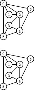
The graph at the top has the Hamilton tour 0-6-4-2-1-3-5-0, which visits each vertex exactly once and returns to the start vertex, but the graph at the bottom has no such tour.
Figure 17.19 Hamilton-tour–search trace
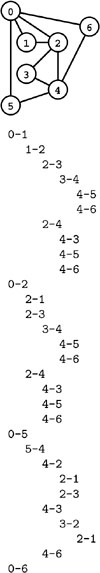
This trace shows the edges checked by Program 17.17 when discovering that the graph shown at the top has no Hamilton tour. For brevity, edges to marked vertices are omitted.
Hamilton tour problem. Is there a cycle that visits every vertex in the graph exactly once?
At first blush, this problem seems to admit a simple solution: We can use the simple modification to the recursive part of the path-finding class that is shown in Program 17.17. But this program is not likely to be useful for many graphs, because its worst-case running time is exponential in the number of vertices in the graph.
Property 17.3 A recursive search for a Hamilton tour could take exponential time.
Proof: Consider a graph where vertex V-1 is isolated and the edges, with the other V − 1 vertices, constitute a complete graph. Program 17.17 will never find a Hamilton path, but it is easy to see by induction that it will examine all of the (V − 1)! paths in the complete graph, all of which involve V − 1 recursive calls. The total number of recursive calls is therefore about V !, or about (V/e) V, which is higher than any constant to the V th power. •
Our implementations Program 17.16 for finding simple paths and Program 17.17 for finding Hamilton paths are extremely similar. If no path exists, both programs terminate when all the elements of the visited vector are set to true. Why are the running times so dramatically different? Program 17.16 is guaranteed to finish quickly because it sets at least one element of the visited vector to 1 each time searchR is called. Program 17.17, on the other hand, can set visited elements back to 0, so we cannot guarantee that it will finish quickly.
When searching for simple paths, in Program 17.16, we know that, if there is a path from v to w, we will find it by taking one of the edges v-t from v, and the same is true for Hamilton paths. But there this similarity ends. If we cannot find a simple path from t to w, then we can conclude that there is no simple path from v to w that goes through t; but the analogous situation for Hamilton paths does not hold. It could be the case that there is no Hamilton path to w that starts with v-t, but there is one that starts with v-x-t for some other vertex x. We have to make a recursive call from t corresponding to every path that leads to it from v. In short, we may have to check every path in the graph.
It is worthwhile to reflect on just how slow a factorial-time algorithm is. If we could process a graph with 15 vertices in 1 second, it would take 1 day to process a graph with 19 vertices, over 1 year for 21 vertices, and over 6 centuries for 23 vertices. Faster computers do not help much, either. A computer that is 200,000 times faster than our original one would still take more than a day to solve that 23-vertex problem. The cost to process graphs with 100 or 1000 vertices is too high to contemplate, let alone graphs of the size that we might encounter in practice. It would take millions of pages in this book just to write down the number of centuries required to process a graph that contained millions of vertices.
In Chapter 5, we examined a number of simple recursive programs that are similar in character to Program 17.17 but that could be drastically improved with top-down dynamic programming. This recursive program is entirely different in character: The number of intermediate results that would have to be saved is exponential. Despite many people doing an extensive amount of work on the problem, no one has been able to find any algorithm that can promise reasonable performance for large (or even medium-sized) graphs.
Figure 17.20 Euler tour and path examples
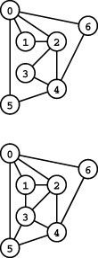
The graph at the top has the Euler tour 0-1-2-0-6-4-3-2-4-5-0, which uses all the edges exactly once. The graph at the bottom no such tour, but it has the Euler path 1-2-0-1-3-4-2-3-5-4-6-0-5.
Now, suppose that we change the restriction from having to visit all the vertices to having to visit all the edges. Is this problem easy, like finding a simple path, or hopelessly difficult, like finding a Hamilton path?
Euler path Is there a path connecting two given vertices that uses each edge in the graph exactly once? The path need not be simple—vertices may be visited multiple times. If the path is from a vertex back to itself, we have the Euler tour problem. Is there a cyclic path that uses each edge in the graph exactly once? We prove in the corollary to Property 17.4 that the path problem is equivalent to the tour problem in a graph formed by adding an edge connecting the two vertices. Figure 17.20 gives two small examples.
This classical problem was first studied by L. Euler in 1736. Indeed, some people trace the origin of the study of graphs and graph theory to Euler’s work on this problem, starting with a special case known as the bridges of Königsberg problem (see Figure 17.21). The Swiss town of Königsberg had seven bridges connecting riverbanks and islands, and people in the town found that they could not seem to cross all the bridges without crossing one of them twice. Their problem amounts to the Euler tour problem.
These problems are familiar to puzzle enthusiasts. They are commonly seen in the form of puzzles where you are to draw a given figure without lifting your pencil from the paper, perhaps under the constraint that you must start and end at particular points. It is natural for us to consider Euler paths when developing graph-processing algorithms, because an Euler path is an efficient representation of the graph (putting the edges in a particular order) that we might consider as the basis for developing efficient algorithms.
Euler showed that it is easy to determine whether or not a path exists, because all that we need to do is to check the degree of each of the vertices. The property is easy to state and apply, but the proof is a tricky exercise in graph theory.
Property 17.4 A graph has an Euler tour if and only if it is connected and all its vertices are of even degree.
Proof: To simplify the proof, we allow self-loops and parallel edges, though it is not difficult to modify the proof to show that this property also holds for simple graphs (see Exercise 17.94).
If a graph has an Euler tour, then it must be connected because the tour defines a path connecting each pair of vertices. Also, any given vertex v must be of even degree because when we traverse the tour (starting anywhere else), we enter v on one edge and leave on a different edge (neither of which appear again on the tour); so the number of edges incident upon v must be twice the number of times we visit v when traversing the tour, an even number.
To prove the converse, we use induction on the number of edges. The claim is certainly true for graphs with no edges. Consider any connected graph that has more than one edge, with all vertices of even degree. Suppose that, starting at any vertex v, we follow and remove any edge, and we continue doing so until arriving at a vertex that has no more edges. This process certainly must terminate, since we delete an edge at every step, but what are the possible outcomes? Figure 17.22 illustrates examples. Immediately, we see that we must end up back at v, because we end at a vertex other than v if and only if that vertex had an odd degree when we started.
One possibility is that we trace the full tour; if so, we are done. Otherwise, all the vertices in the graph that remains have even degree, but it may not be connected. Still, each connected component has an Euler tour by the inductive hypothesis. Moreover, the cyclic path just removed connects those tours together into an Euler tour for the original graph: traverse the cyclic path, taking detours to do the Euler tours for the connected components. Each detour is a proper Euler tour that takes us back to the vertex on the cyclic path where it started. Note that a detour may touch the cyclic path multiple times (see Exercise 17.98). In such a case, we take the detour only once (say, when we first encounter it). •
Corollary A graph has an Euler path if and only if it is connected and exactly two of its vertices are of odd degree.
Proof: This statement is equivalent to Property 17.4 in the graph formed by adding an edge connecting the two vertices of odd degree (the ends of the path).•
Therefore, for example, there is no way for anyone to traverse all the bridges of Königsberg in a continuous path without retracing their steps, since all four vertices in the corresponding graph have odd degree (see Figure 17.21).
Figure 17.21 Bridges of Königsberg
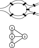
A well-known problem studied by Euler has to do with the town of Königsberg, in which there is an island at the point where the river Pregel forks. There are seven bridges connecting the island with the two banks of the river and the land between the forks, as shown in the diagram at top. Is there a way to cross the seven bridges in a continuous walk through the town, without recrossing any of them? If we label the island 0, the banks 1 and 2, and the land between the forks 3 and define an edge corresponding to each bridge, we get the multigraph shown at the bottom. The problem is to find a path through this graph that uses each edge exactly once.
Figure 17.22 Partial tours
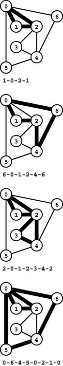
Following edges from any vertex in a graph that has an Euler tour always takes us back to that vertex, as shown in these examples. The cycle does not necessarily use all the edges in the graph.
As discussed in Section 17.5, we can find all the vertex degrees in time proportional to E for the adjacency-lists or set-of-edges representation and in time proportional to V2 for the adjacency-matrix representation, or we can maintain a vertex-indexed vector with vertex degrees as part of the graph representation (see Exercise 17.42). Given the vector, we can check whether Property 17.4 is satisfied in time proportional to V. Program 17.18 implements this strategy and demonstrates that determining whether a given graph has an Euler path is an easy computational problem. This fact is significant because we have little intuition to suggest that the problem should be easier than determining whether a given graph has a Hamilton path.
Now, suppose that we actually wish to find an Euler path. We are treading on thin ice because a direct recursive implementation (find a path by trying an edge and then making a recursive call to find a path for the rest of the graph) will have the same kind of factorial-time performance as Program 17.17. We expect not to have to live with such performance because it is so easy to test whether a path exists, so we seek a better algorithm. It is possible to avoid factorial-time blowup with a fixed-cost test for determining whether or not to use an edge (rather than unknown costs from the recursive call), but we leave this approach as an exercise (see Exercises 17.96 and 17.97).
Another approach is suggested by the proof of Property 17.4. Traverse a cyclic path, deleting the edges encountered and pushing onto a stack the vertices that it encounters, so that (i) we can trace back along that path, printing out its edges, and (ii) we can check each vertex for additional side paths (which can be spliced into the main path). This process is illustrated in Figure 17.23.
Program 17.19 is an implementation along these lines. It assumes that an Euler path exists, and it destroys its local copy of the graph; thus, it is important that the Graph class that this program uses have a copy constructor that creates a completely separate copy of the graph. The code is tricky—novices may wish to postpone trying to understand it until gaining more experience with graph-processing algorithms in the next few chapters. Our purpose in including it here is to illustrate that good algorithms and clever implementations can be very effective for solving some graph-processing problems.
Property 17.5 We can find an Euler tour in a graph, if one exists, in linear time.
We leave a full induction proof as an exercise (see Exercise 17.100). Informally, after the first call on path, the stack contains a path from v to w, and the graph that remains (after removal of isolated vertices) consists of the smaller connected components (sharing at least one vertex with the path so far found) that also have Euler tours. We pop isolated vertices from the stack and use path to find Euler tours that
contain the nonisolated vertices, in the same manner. Each edge in the graph is pushed onto (and popped from) the stack exactly once, so the total running time is proportional to E.•
Despite their appeal as a systematic way to traverse all the edges and vertices, we rarely use Euler tours in practice because few graphs have them. Instead, we typically use depth-first search to explore
Figure 17.23 Euler tour by removing cycles
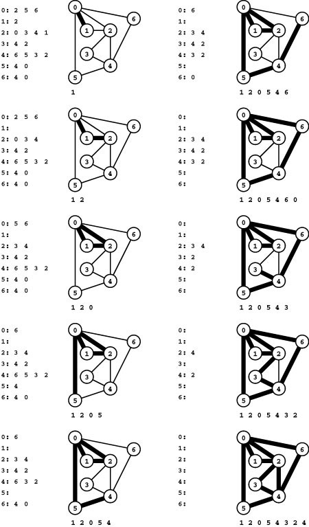
This figure shows how Program 17.19 discovers an Euler tour from 0 back to 0 in a sample graph. Thick black edges are those on the tour, the stack contents are listed below each diagram, and adjacency lists for the non-tour edges are shown at left.
First, the program adds the edge 0-1 to the tour and removes it from the adjacency lists (in two places) (top left, lists at left). Second, it adds 1-2 to the tour in the same way (left, second from top). Next, it winds up back at 0 but continues to do another cycle 0-5-4-6-0, winding up back at 0 with no more edges incident upon 0 (right, second from top). Then it pops the isolated vertices 0 and 6 from the stack until 4 is at the top and starts a tour from 4 (right, third from from top), which takes it to 3, 2, and back to 4, whereupon it pops all the now-isolated vertices 4, 2, 3, and so forth. The sequence of vertices popped from the stack defines the Euler tour 0-6-4-2-3-4-5-0-2-1-0 of the whole graph.
graphs, as described in detail in Chapter 18. Indeed, as we shall see, doing depth-first search in an undirected graph amounts to computing a two-way Euler tour: a path that traverses each edge exactly twice, once in each direction.
In summary, we have seen in this section that it is easy to find simple paths in graphs, that it is even easier to know whether we can tour all the edges of a large graph without revisiting any of them (by just checking that all vertex degrees are even), and that there is even a clever algorithm to find such a tour; but that it is practically impossible to know whether we can tour all the graph’s vertices without revisiting any. We have simple recursive solutions to all these problems, but the potential for exponential growth in the running time renders some of the solutions useless in practice. Others provide insights that lead to fast practical algorithms.
This range of difficulty among apparently similar problems that is illustrated by these examples is typical in graph processing, and is fundamental to the theory of computing. As discussed briefly in Section 17.8 andindetail inPart 8, we must acknowledge what seems to be an insurmountable barrier between problems that seem to require exponential time (such as the Hamilton tour problem and many other commonly encountered problems) and problems for which we know algorithms that can guarantee to find a solution in polynomial time (such as the Euler tour problem and many other commonly encountered problems). In this book, our primary objective is to develop efficient algorithms for problems in the latter class.
Exercises
• 17.85 Show, in the style of Figure 17.17, the trace of recursive calls (and vertices that are skipped) when Program 17.16 finds a path from 0 to 5 in the graph
3-7 1-4 7-8 0-5 5-2 3-8 2-9 0-6 4-9 2-6 6-4.
17.86 Modify the recursive function in Program 17.16 to print out a trace like Figure 17.17, using a global variable as described in the text.
17.87 Do Exercise 17.86 by adding an argument to the recursive function to keep track of the depth.
• 17.88 Using the method described in the text, give an implementation of sPATH that provides a public member function that calls a client-supplied function for each edge on a path from v to w, if any such path exists.
• 17.89 Modify Program 17.16 such that it takes a third argument d and tests the existence of a path connecting u and v of length greater than d. In particular, search(v, v, 2) should be nonzero if and only if v is on a cycle.
• 17.90 Run experiments to determine empirically the probability that Program 17.16 finds a path between two randomly chosen vertices for various graphs (see Exercises 17.63–76) and to calculate the average length of the paths found for each type of graph.
• 17.91 Consider the graphs defined by the following four sets of edges:
0-1 0-2 0-3 1-3 1-4 2-5 2-9 3-6 4-7 4-8 5-8 5-9 6-7 6-9 7-8
0-1 0-2 0-3 1-3 0-3 2-5 5-6 3-6 4-7 4-8 5-8 5-9 6-7 6-9 8-8
0-1 1-2 1-3 0-3 0-4 2-5 2-9 3-6 4-7 4-8 5-8 5-9 6-7 6-9 7-8
4-1 7-9 6-2 7-3 5-0 0-2 0-8 1-6 3-9 6-3 2-8 1-5 9-8 4-5 4-7.
Which of these graphs have Euler tours? Which of them have Hamilton tours?
• 17.92 Give necessary and sufficient conditions for a directed graph to have a (directed) Euler tour.
17.93 Prove that every connected undirected graph has a two-way Euler tour.
17.94 Modify the proof of Property 17.4 to make it work for graphs with parallel edges and self-loops.
• 17.95 Show that adding one more bridge could give a solution to the bridges-of-Königsberg problem.
• 17.96 Prove that a connected graph has an Euler path from v to w only if it has an edge incident on v whose removal does not disconnect the graph (except possibly by isolating v).
• 17.97 Use Exercise 17.96 to develop an efficient recursive method for finding an Euler tour in a graph that has one. Beyond the basic graph ADT functions, you may use the classes from this chapter that can give vertex degrees (see Program 17.11) and test whether a path exists between two given vertices (see Program 17.16). Implement and test your program for both sparse and dense graphs.
• 17.98 Give an example where the graph remaining after the first call to path in Program 17.19 is not connected (in a graph that has an Euler tour).
• 17.99 Describe how to modify Program 17.19 so that it can be used to detect whether or not a given graph has an Euler tour, in linear time.
17.100 Give a complete proof by induction that the linear-time Euler tour algorithm described in the text and implemented in Program 17.19 properly finds an Euler tour.
• 17.101 Find the number of V -vertex graphs that have an Euler tour, for as large a value of V as you can feasibly afford to do the computation.
• 17.102 Run experiments to determine empirically the average length of the path found by the first call to path in Program 17.19 for various graphs (see Exercises 17.63–76). Calculate the probability that this path is cyclic.
• 17.103 Write a program that computes a sequence of 2n + n - 1 bits in which no two pairs of n consecutive bits match. (For example, for n = 3, the sequence 0001110100 has this property.)Hint: Find a Euler tour in a de Bruijn digraph.
• 17.104 Show, in the style of Figure 17.19, the trace of recursive calls (and vertices that are skipped), when Program 17.16 finds a Hamilton tour in the graph
3-7 1-4 7-8 0-5 5-2 3-8 2-9 0-6 4-9 2-6 6-4.
17.105 Modify Program 17.17 to print out the Hamilton tour if it finds one.
• 17.106 Find a Hamilton tour of the graph
1-2 5-2 4-2 2-6 0-8 3-0 1-3 3-6 1-0 1-4 4-0 4-6 6-5 2-6
6-9 9-0 3-1 4-3 9-2 4-9 6-9 7-9 5-0 9-7 7-3 4-5 0-5 7-8
or show that none exists.
••17.107 Determine how many V -vertex graphs have a Hamilton tour, for as large a value of V as you can feasibly afford to do the computation.
17.8 Graph-Processing Problems
Armed with the basic tools developed in this chapter, we consider in Chapters 18 through 22 a broad variety of algorithms for solving graph-processing problems. These algorithms are fundamental ones and are useful in many applications, but they serve as only an introduction to the subject of graph algorithms. Many interesting and useful algorithms have been developed that are beyond the scope of this book, and many interesting problems have been studied for which good algorithms have still not yet been invented.
As is true in any domain, the first challenge that we face in addressing a new graph-processing problem is determining how difficult it is to solve. For graph processing, this decision can be far more difficult than we might imagine, even for problems that appear to be simple to solve. Moreover, our intuition is not always helpful in distinguishing easy problems from difficult or hitherto unsolved ones. In this section, we describe briefly important classical problems and the state of our knowledge of them.
Given a new graph-processing problem, what type of challenge do we face in developing an implementation to solve it? The unfortunate truth is that there is no good method to answer this question for any problem that we might encounter, but we can provide a general description of the difficulty of solving various classical graph-processing problems. To this end, we will roughly categorize the problems according to the difficulty of solving them, as follows:
• Easy
• Tractable
• Intractable
• Unknown
These terms are intended to convey information relative to one another and to the current state of knowledge about graph algorithms.
As indicated by the terminology, our primary reason for categorizing problems in this way is that there are many graph problems, such as the Hamilton tour problem, that no one knows how to solve efficiently. We will eventually see (in Part 8) how to make that statement meaningful in a precise technical sense; at this point, we can at least be warned that we face significant obstacles to writing an efficient program to solve these problems.
We defer full context on many of the graph-processing problems until later in the book. Here, we present brief statements that are easily understood, in order to introduce the general issue of classifying the difficulty of graph-processing problems.
An easy graph-processing problem is one that can be solved by the kind of elegant and efficient short programs to which we have grown accustomed in Parts 1 through 4. We often find the running time to be linear in the worst case, or bounded by a small-degree polynomial in the number of vertices or the number of edges. Generally, as we have done in many other domains, we can establish that a problem is easy by developing a brute-force solution that, although it may be too slow for huge graphs, is useful for small and even intermediate-sized problems. Then, once we know that the problem is easy, we look for efficient solutions that we might use in practice and try to identify the best among those. The Euler tour problem that we considered in Section 17.7 is a prime example of such a problem, and we shall see many others in Chapters 18 through 22 including, most notably, the following.
Simple connectivity Is a given graph connected? That is, is there a path connecting every pair of vertices? Is there a cycle in the graph, or is it a forest? Given two vertices, are they on a cycle? We first considered these basic graph-processing question in Chapter 1. We consider numerous solutions to such problems in Chapter 18. Some are trivial to implement in linear time; others have rather sophisticated linear-time solutions that bear careful study.
Strong connectivity in digraphs Is there a directed path connecting every pair of vertices in a digraph? Given two vertices, are they connected by directed paths in both directions (are they on a directed cycle)? Implementing efficient solutions to these problems is a much more challenging task than for the corresponding simple-connectivity problem in undirected graphs, and much of Chapter 19 is devoted to studying them. Despite the clever intricacies involved in solving them, we classify the problems as easy because we can write a compact, efficient, and useful implementation.
Transitive closure What set of vertices can be reached by following directed edges from each vertex in a digraph? This problem is closely related to strong connectivity and to other fundamental computational problems. We study classical solutions that amount to a few lines of code in Chapter 19.
Minimum spanning tree In a weighted graph, find a minimum-weight set of edges that connects all the vertices. This is one of the oldest and best-studied graph-processing problems; Chapter 20 is devoted to the study of various classical algorithms to solve it. Researchers still seek faster algorithms for this problem.
Single-source shortest paths What are the shortest paths connecting a given vertex v with each other vertex in a weighted digraph (network)? Chapter 21 is devoted to the study of this problem, which is extremely important in numerous applications. The problem is decidedly not easy if edge weights can be negative.
A tractable graph-processing problem is one for which an algorithm is known whose time and space requirements are guaranteed to be bounded by a polynomial function of the size of the graph (V + E ). All easy problems are tractable, but we make a distinction because many tractable problems have the property that developing an efficient practical program to solve is an extremely challenging, if not impossible, task. Solutions may be too complicated to present in this book, because implementations might require hundreds or even thousands of lines of code. The following examples are two of the most important problems in this class.
Planarity Can we draw a given graph without any of the lines that represent edges intersecting? We have the freedom to place the vertices anywhere, so we can solve this problem for many graphs, but it is impossible to solve for many other graphs. A remarkable classical result known as Kuratowski’s theorem provides an easy test for determining whether a graph is planar: it says that the only graphs that cannot be drawn with no edge intersections are those that contain some subgraph that, after removing vertices of degree 2, is isomorphic to one of the graphs in Figure 17.24. A straightforward implementation of that test, even without taking the vertices of degree 2 into consideration, would be too slow for large graphs (see Exercise 17.110), but in 1974 R. Tarjan developed an ingenious (but intricate) algorithm for solving the problem in linear time, using a depth-first search scheme that extends those that we consider in Chapter 18. Tarjan’s algorithm does not necessarily give a practical layout; it just certifies that a layout exists. As discussed in Section 17.1, developing a visually pleasing layout in applications where vertices do not necessarily relate directly to the physical world has turned out to be a challenging research problem.
Matching Given a graph, what is the largest subset of its edges with the property that no two are connected to the same vertex? This classical problem is known to be solvable in time proportional to a polynomial function of V and E, but a fast algorithm that is suitable for huge graphs is still an elusive research goal. The problem is easier to solve when restricted in various ways. For example, the problem of matching students to available positions in selective institutions is an example of bipartite matching: We have two different types of vertices (students and institutions) and we are concerned with only those edges that connect a vertex of one type with a vertex of the other type. We see a solution to this problem in Chapter 22.
The solutions to some tractable problems have never been written down as programs, or have running times so high that we could not contemplate using them in practice. The following example is in this class. It also demonstrates the capricious nature of the mathematical reality of the difficulty of graph processing.
Figure 17.24 Forbidden subgraphs in planar graphs
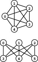
Neither of these graphs can be drawn in the plane without intersecting edges, nor can any graph that contains either of these graphs as a subgraph (after we remove vertices of degree two); but all other graphs can be so drawn.
Even cycles in digraphs Does a given digraph have a cycle of even length? This question would seem simple to resolve because the corresponding question for undirected graphs is easy to solve (see Section 18.4), as is the question of whether a digraph has a cycle of odd length. However, for many years, the problem was not sufficiently well understood for us even to know whether or not there exists an efficient algorithm for solving it (see reference section). A theorem establishing the existence of an efficient algorithm was proved in 1999, but the method is so complicated that no mathematician or programmer would attempt to implement it.
One of the important themes of Chapter 22 is that many tractable graph problems are best handled by algorithms that can solve a whole class of problems in a general setting. The shortest-paths algorithms of Chapter 21, the network-flow algorithms of Chapter 22, and the powerful network-simplex algorithm of Chapter 22 are capable of solving many graph problems that otherwise might present a significant challenge. Examples of such problems include the following.
Assignment This problem, also known as bipartite weighted matching, is to find a perfect matching of minimum weight in a bipartite graph. It is easily solved with network-flow algorithms. Specific methods that attack the problem directly are known, but they have been shown to be essentially equivalent to network-flow solutions.
General connectivity What is the minimum number of edges whose removal will separate a graph into two disjoint parts (edge connectivity)? What is the minimum number of vertices whose removal will separate a graph into two disjoint parts (vertex connectivity)? As we see in Chapter 22, these problems, although difficult to solve directly, can both be solved with network-flow algorithms.
Mail carrier Given a graph, find a tour with a minimal number of edges that uses every edge in the graph at least once (but is allowed to use edges multiple times). This problem is much more difficult than the Euler tour problem but much less difficult than the Hamilton tour problem.
The step from convincing yourself that a problem is tractable to providing software that can be used in practical situations can be a large step, indeed. On the one hand, when proving that a problem is tractable, researchers tend to brush past numerous details that have to be dealt with in an implementation; on the other hand, they have to account for numerous potential situations even though they may not arise in practice. This gap between theory and practice is particularly acute when investigators are considering graph algorithms, both because mathematical research is filled with deep results describing a bewildering variety of structural properties that we may need to take into account when processing graphs, and because the relationships between those results and the properties of graphs that arise in practice are little understood. The development of general schemes such as the network-simplex algorithm has been an extremely effective approach to dealing with such problems.
An intractable graph-processing problem is one for which there is no known algorithm that is guaranteed to solve the problem in a reasonable amount of time. Many such problems have the characteristic that we can use a brute-force method where we can try all possibilities to compute the solution—we consider them to be intractable because there are far too many possibilities to consider. This class of problems is extensive and includes many important problems that we would like to know how to solve. The term NP-hard describes the problems in this class. Most experts believe that no efficient algorithms exist for these problems. We consider the bases for this terminology and this belief in more detail in Part 8. The Hamilton path problem that we discussed in Section 17.7 is a prime example of an NP-hard graph-processing problem, as are those on the following list.
Longest path What is the longest simple path connecting two given vertices in a graph? Despite its apparent similarity to shortest-paths problems, this problem is a version of the Hamilton tour problem, and is NP-hard.
Colorability Is there a way to assign one of k colors to each of the vertices of a graph such that no edge connects two vertices of the same color? This classical problem is easy for k = 2 (see Section 18.4), but it is NP-hard for k =3.
Independent set What is the size of the largest subset of the vertices of a graph with the property that no two are connected by an edge? Just as we saw when contrasting the Euler and Hamilton tour problems, this problem is NP-hard, despite its apparent similarity to the matching problem, which is solvable in polynomial time.
Clique What is size of the largest clique (complete subgraph) in a given graph? This problem generalizes part of the planarity problem, because if the largest clique has more than four nodes, the graph is not planar.
These problems are formulated as existence problems—we are asked to determine whether or not a particular subgraph exists. Some of the problems ask for the size of the largest subgraph of a particular type, which we can do by framing an existence problem where we test for the existence of a subgraph of size k that satisfies the property of interest, then use binary search to find the largest. In practice, we actually often want to find a complete solution, which is potentially much harder to do. Four example, the famous four-color theorem tells us that it is possible use just four colors to color all the vertices of a planar graph such that no edge connects two vertices of the same color. But the theorem does not tell us how to do so for a particular planar graph: knowing that a coloring exists does not help us find a complete solution to the problem. Another famous example is the traveling salesperson problem, which asks us to find the minimum-length tour through all the vertices of a weighted graph. This problem is related to the Hamilton path problem, but it is certainly no easier: if we cannot find an efficient solution to the Hamilton path problem, we cannot expect to find one for the traveling salesperson problem. As a rule, when faced with difficult problems, we work with the simplest version that we cannot solve. Existence problems are within the spirit of this rule, but they also play an essential role in the theory, as we shall see in Part 8.
The problems just listed are but a few of the thousands of NP-hard problems that have been identified. They arise in all types of computational applications, as we shall discuss in Part 8; they are particularly prevalent in graph processing, so we have to be aware of their existence throughout this book.
Note that we are insisting that our algorithms guarantee efficiency, in the worst case. Perhaps we should instead settle for algorithms that are efficient for typical inputs (but not necessarily in the worst case). Similarly, many of the problems involve optimization. Perhaps we should instead settle for a long path (not necessarily the longest) or a large clique (not necessarily the maximum). For graph processing, it might be easy to find a good answer for graphs that arise in practice, and we may not even be interested in looking for an algorithm that could find an optimal solution in fictional graphs that we will never see. Indeed, intractable problems can often be attacked with straightforward or general-purpose algorithms similar to Program 17.17 that, although they have exponential running time in the worst case, can quickly find a solution (or a good approximation) for specific problem instances that arise in practice. We would be reluctant to use a program that will crash or produce a bad answer for certain inputs, but we do sometimes find ourselves using programs that run in exponential time for certain inputs. We consider this situation in Part 8.
There are also many research results proving that various intractable problems remain intractable even when we relax various restrictions. Moreover, there are many specific practical problems that we cannot solve because no one knows a sufficiently fast algorithm. In this part of the book, we will label problems NP-hard when we encounter them and interpret this label as meaning, at the very least, that we are not going to expect to find efficient algorithms to solve them and that we are not going to attack them without using advanced techniques of the type discussed in Part 8 (except perhaps to use brute-force methods to solve tiny problems).
There are some graph-processing problems whose difficulty is unknown. Neither is there an efficient algorithm known for them, nor are they known to be NP-hard. It is possible, as our knowledge of graph-processing algorithms and properties of graphs expands, that some of these problems will turn out to be tractable, or even easy. The following important natural problem, which we have already encountered (see Figure 17.2), is the best-known problem in this class.
Graph isomorphism Can we make two given graphs identical by renaming vertices? Efficient algorithms are known for this problem for many special types of graphs, but the difficulty of the general problem remains open.
The number of significant problems whose intrinsic difficulty is unknown is very small in comparison to the other categories that we have considered, because of intense research in this field over the past several decades. Certain problems in this class, such as graph isomorphism, are of immense practical interest; other problems in this class are of significance primarily by virtue of having resisted classification.
Table 17.2 Difficulty of classical graph-processing problems
This table summarizes the discussion in the text about the relative difficulty of various classical graph-processing problems, comparing them in rough subjective terms. These examples indicate not only the range of difficulty of the problems but also that classifying a given problem can be a challenging task.
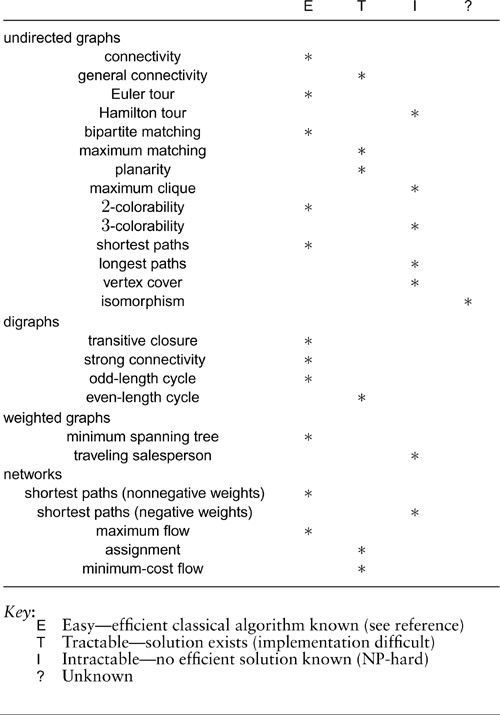
For the class of easy algorithms, we are used to the idea of comparing algorithms with different worst-case performance characteristics and trying to predict performance through analysis and empirical tests. For graph processing, these tasks are particularly challenging because of the difficulty of characterizing the types of graphs that might arise in practice. Fortunately, many of the important classical algorithms have optimal or near-optimal worst-case performance, or have a running time that depends on only the number of vertices and edges, rather than on the graph structure; we thus can concentrate on streamlining implementations and still can predict performance with confidence.
In summary, there is a wide spectrum of problems and algorithms known for graph processing. Table 17.2 summarizes some of the information that we have discussed. Every problem comes in different versions for different types of graphs (directed, weighted, bipartite, planar, sparse, dense), and there are thousands of problems and algorithms to consider. We certainly cannot expect to solve every problem that we might encounter, and some problems that appear to be simple are still baffling the experts. Despite a natural a priori expectation that we should have no problem distinguishing easy problems from intractable ones, the many examples that we have discussed illustrate that placing a problem even into these rough categories can turn into a significant research challenge.
As our knowledge about graphs and graph algorithms expands, given problems may move among these categories. Despite a flurry of research activity in the 1970s and intensive work by many researchers since then, the possibility still remains that all the problems that we are discussing will someday be categorized as “easy” (solvable by an algorithm that is compact, efficient, and possibly ingenious).
Having developed this context, we shall press on to consider numerous useful graph-processing algorithms. Problems that we can solve do arise often, the graph algorithms that we study serve well in a great variety of applications, and these algorithms serve as the basis for attacking numerous other problems that we need to handle even if we cannot guarantee efficient solutions.
Exercises
• 17.108 Prove that neither of the two graphs depicted in Figure 17.24 is planar.
17.109 Write a graph ADT client that determines whether or not a graph contains one of the graphs depicted in Figure 17.24, using a brute-force algorithm where you test all possible subsets of five vertices for the clique and all possible subsets of six vertices for the complete bipartite graph. Note: This test does not suffice to show whether the graph is planar, because it ignores the condition that removing vertices of degree 2 in some subgraph might give one of the two forbidden subgraphs.
17.110 Give a drawing of the graph
3-7 1-4 7-8 0-5 5-2 3-0 2-9 0-6 4-9 2-6
6-4 1-5 8-2 9-0 8-3 4-5 2-3 1-6 3-5 7-6
that has no intersecting edges, or prove that no such drawing exists.
17.111 Find a way to assign three colors to the vertices of the graph
3-7 1-4 7-8 0-5 5-2 3-0 2-9 0-6 4-9 2-6
6-4 1-5 8-2 9-0 8-3 4-5 2-3 1-6 3-5 7-6
such that no edge connects two vertices of the same color, or show that it is not possible to do so.
17.112 Solve the independent-set problem for the graph
3-7 1-4 7-8 0-5 5-2 3-0 2-9 0-6 4-9 2-6
6-4 1-5 8-2 9-0 8-3 4-5 2-3 1-6 3-5 7-6.
17.113 What is the size of the largest clique in a de Bruijn graph of order n?