Chapter 14
Trading Decisions
What Makes Trading So Difficult
In this section I will discuss why one of the most common approaches to trading is dead wrong. I'll also explain what makes it so appealing and why it will continue to be difficult to resist, even after I prove to you that it is irrational.
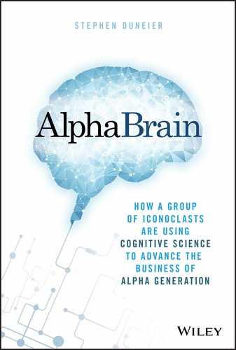
Let's begin with the basics of investing. You form a view and with it come expectations. See Figure 14.1 for an example. In this case the investor is bullish.
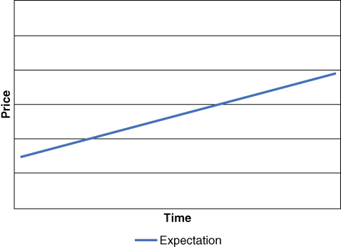
Figure 14.1 A bullish investor
Of course, we aren't so naive as to believe that anything will move in such a straight line, so we have a range within which we expect it to trade (see Figure 14.2).
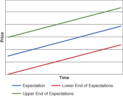
Figure 14.2 Expected trading range
As time goes by the spot price ebbs and flows, sometimes moving higher confirming your view, while other times it moves lower calling your view into question (see Figure 14.3). When we look back on an asset's price action it actually appears to be this clear cut, and the job, with the benefit of hindsight, seems like it really is that simple. The reality, however, is quite different.
Figure 14.3 Price action
Let's examine what happens when the price moves down toward the lower end of your expectations (see Figure 14.4). As long as all the reasons behind your establishment of the view remain in place, the only thing that has changed is the risk/reward. The closer spot gets to the lower end of your expectations, the more attractive the trade becomes from a risk/reward perspective. As a result, it is the point at which the position should be at its maximize size. Think about that for just a moment. I am suggesting that you should max out your position size at the exact moment when your confidence is likely to be at its lowest. Why would it be low? Well, something must have happened to drive the price lower and that something is likely to be what everyone is talking about at that moment. It is also evidence against a bullish view. Why else would it have pushed the price lower?

Figure 14.4 Price moves down
So, in that moment you are likely to be bombarded with all the reasons you should not be bullish. The guy sitting next to you, the talking heads on TV, analysts and salespeople are all essentially telling you why your view and accompanying expectations are wrong.
Assuming your investment process is valid and you have identified up front what the important factors are that affect your view (the signals), then everything else is essentially noise as it relates to this position. Therefore, it shouldn't matter what the guy next to you or anyone else has to say. You should feel as confident in your view and expectations as you did on day 1. As a result, you should take full advantage of the move down and max out your position size.
Why is it that this moment creates so many problems for investors? Well, most don't invite cognitive strain up front during the planning phase of the trade. Most don't put in the effort to identify what represents a signal when they first establish the view and set their expectations. Therefore, when the noise is released, everyone is talking about it and it pushes the price lower, it becomes difficult to determine whether it is, in fact, signal or noise. You begin to question your view. Your confidence wanes. So, instead of sizing up as you should, you sit and wait for confirmation, or even worse, you cut it.
Now let's examine what happens as you approach the upper end of your expectations (see Figure 14.5). Your confidence is at its peak. Everything, especially price action, is supportive of your view. Everyone who told you your view was wrong is now explaining to you not only why it has gone up, but why it will make new highs and break out to the upside. Momentum traders have received confirmation and are beginning to really load up. You are giddy with excitement, knowing that you were right all along. The guy sitting next to you is now singing your praises, patting you on the back for being so amazing. He too has loaded up and is feeding you a constant diet of evidence confirming your view including information that you hadn't identified as signal when you first established the position. (Yes, even confirming evidence can be noise.) With everyone talking about it and so many profiting you begin to worry that others, particularly those who were arguing that it would breakout to the downside just days earlier, will profit more from your idea than you will. That is what makes it so difficult to begin unwinding the position, but that is exactly what you should be doing as the risk/reward has flipped to the opposite extreme. Being so close to the upper end of your expectations and so far from the lower end means your risk is now much greater than your potential reward. As a result your position size should be at or near zero. Take a second to contemplate what I am saying. At the moment your confidence is at its highest, your position size should be at its lowest. It sounds and feels counterintuitive, which is why it is so difficult to make the rational decision.
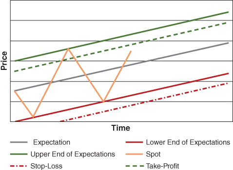
Figure 14.5 Peak confidence
What do most traders do instead of unwinding the position? They move their stop‐loss up, thereby effectively rebalancing the risk/reward. While it may appear rational, it is not. The reason is that the upper and lower expectation bands represent discrete moments. What that means is the probability of spot trading just above the upper band is disproportionately lower than the probability of it trading just below it (see Figure 14.6). So, if you want a high probability that your take‐profit will be hit, you should set it below the upper band.
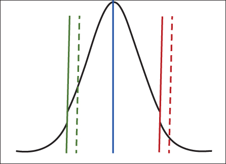
Figure 14.6 Spot trading probability
On the other hand, the probability of spot trading just below the lower end of your expectations is disproportionately lower than the probability of it trading just above the lower end. Therefore, if you don't want to be stopped out while your view is still in effect, you should set your stop‐loss just below the lower end of your expectations. If you were to raise your stop‐loss with the objective of rebalancing the risk/reward, you are shifting the probability of triggering that stop‐loss from very low to very high (see Figure 14.7). So, while you are reducing the magnitude of your potential downside, you are significantly increasing the likelihood of actually realizing that loss.

Figure 14.7 The effect of changing a stop‐loss
What I am saying is that the rational decision would have you reduce your position when momentum traders are loading up, and loading up when they are stopping out. If you are an investor who expresses a view based on fundamentals, momentum trading is incompatible with your approach. In fact, it is downright corrosive. Do it often enough and you'll find yourself saying, “I got my view right, I just didn't make any money on it.”
The Freedom of a Straightjacket
I often hear investors talk about wanting to remain agile, not wanting to be straightjacketed. They believe it's important to be able to react to new information as it becomes available, to reassess the situation as it unfolds and adapt. Very often what they're really saying is they don't want to have to contemplate all of the likely future events, variables, and outcomes that can affect their investments today. They'd rather deal with them as they occur. However, decades of studies in the cognitive sciences suggest that this is a bad idea. By delaying the hard decisions you are avoiding cognitive strain in favor of maintaining cognitive ease. Factors such as losses, gains, and a whole host of emotional triggers are likely to skew your objectivity in that future moment, leaving you with the task of making difficult decisions at a time when extraneous factors, the kind that tend to create bias and result in mistakes, come to the fore.
In the typical “agile” process, decisions are made with the benefit of new information, but also under heightened emotions, increased time constraints, and bias‐inducing influences, like P&L. This reduces the weighting that the new information itself can have on the decision (see Figure 14.8). If instead, we can identify the important information ahead of time, its possible effects, and the resulting adjustment you should make to your forward expectations, then there is no decision to be made in that future moment. It can be made ahead of time in a moment of greater objectivity and lucidity thereby increasing the odds of a better decision.

Figure 14.8 Factors in a decision
Let's use a decision tree to see how this works. Imagine you are contemplating going long in XYZ stock. The catalyst for your potential investment is an impending court ruling. Having done your research you believe the probability of a favorable ruling is 80%. If the ruling does turn out to be favorable, you believe the stock has an 80% chance of trading to $30 and a 20% chance of dropping to $10. If it turns out to be unfavorable, the odds flip (see Figure 14.9). Based on the probabilities you have assigned as a result of your research, and the expected profit/loss in each scenario, when you fold back your decision tree, you come to the conclusion that you should purchase XYZ stock.

Figure 14.9 Initial decision tree (left) compared with probability‐guided decision tree (right)
It's likely that the analysis to this point isn't very different from what goes on in your own head. You've done it so many times over your career you probably don't see the need to take the time to lay out your thoughts on a decision tree or write down your expectations as they exist today. You believe that your expectations (i.e. probabilities assigned) today will remain constant, requiring adjustment only when new information is produced. You will reassess the situation after the ruling comes out.
If you read that last sentence without skipping a beat you've already made a mistake. You see, in your initial analysis, the one that led you to purchase XYZ ahead of the ruling, you set your expectations for the valuation of XYZ given that the ruling was favorable. Therefore, any adjustment to your “post‐ruling expectations” after the ruling is announced will be the result of bias, not the ruling itself.
Prior to the announcement, you believed there was a 68% chance that the stock would trade at $30 (80% chance in the case of a favorable ruling + 20% chance if it were unfavorable.) See Table 14.1. Once the ruling is announced, the only thing in your decision tree that should change is the odds of a favorable versus unfavorable ruling (see Figure 14.10). Strictly as a result of that adjustment your expectation of achieving a loss on the investment has dropped from 32% down to just 20%. No flexibility or adjustment in the moment is necessary. The decision you made initially is the only one you need to make. If you raise your price expectation based solely on the fact that the ruling was favorable you're making a mistake, likely the result of a cognitive bias.
Table 14.1 Prior to court ruling
| Stock Price | Expected Return | Prob of Upper Tgt | Rtn at Upper Tgt | Prob of Lower Expec | Rtn at Lower Expec | Max Downside | Notional |
| 30 | −21.33% | 68% | 0.0% | 32% | −66.7% | −1,000,000 | 1,500,000 |
| 29 | −18.00% | 68% | 3.3% | 32% | −63.3% | −1,000,000 | 1,578,947 |
| 28 | −14.67% | 68% | 6.7% | 32% | −60.0% | −1,000,000 | 1,666,667 |
| 27 | −11.33% | 68% | 10.0% | 32% | −56.7% | −1,000,000 | 1,764,706 |
| 26 | −8.00% | 68% | 13.3% | 32% | −53.3% | −1,000,000 | 1,875,000 |
| 25 | −4.67% | 68% | 16.7% | 32% | −50.0% | −1,000,000 | 2,000,000 |
| 24 | −1.33% | 68% | 20.0% | 32% | −46.7% | −1,000,000 | 2,142,857 |
| 23 | 2.00% | 68% | 23.3% | 32% | −43.3% | −1,000,000 | 2,307,692 |
| 22 | 5.33% | 68% | 26.7% | 32% | −40.0% | −1,000,000 | 2,500,000 |
| 21 | 8.67% | 68% | 30.0% | 32% | −36.7% | −1,000,000 | 2,727,273 |
| 20 | 12.00% | 68% | 33.3% | 32% | −33.3% | −1,000,000 | 3,000,000 |
| 19 | 15.33% | 68% | 36.7% | 32% | −30.0% | −1,000,000 | 3,333,333 |
| 18 | 18.67% | 68% | 40.0% | 32% | −26.7% | −1,000,000 | 3,750,000 |
| 17 | 22.00% | 68% | 43.3% | 32% | −23.3% | −1,000,000 | 4,285,714 |
| 16 | 25.33% | 68% | 46.7% | 32% | −20.0% | −1,000,000 | 5,000,000 |
| 15 | 28.67% | 68% | 50.0% | 32% | −16.7% | −1,000,000 | 6,000,000 |
| 14 | 32.00% | 68% | 53.3% | 32% | −13.3% | −1,000,000 | 7,500,000 |
| 13 | 35.33% | 68% | 56.7% | 32% | −10.0% | −1,000,000 | 10,000,000 |
| 12 | 38.67% | 68% | 60.0% | 32% | −6.7% | −1,000,000 | 15,000,000 |
| 11 | 42.00% | 68% | 63.3% | 32% | −3.3% | −1,000,000 | 30,000,000 |
| 10 | 45.33% | 68% | 66.7% | 32% | 0.0% | −1,000,000 | 0 |
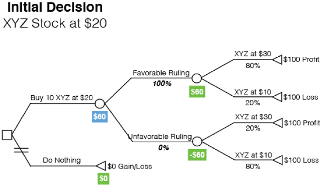
Figure 14.10 Post‐announcement decision tree
Of course, given that a great amount of uncertainty has been removed the expected return on the investment has changed (even though the price target hasn't). Therefore, it makes sense to reassess the investment from this point forward. Perhaps, it is wise to double down. I know what some of you are thinking. So you do have to make a decision in the moment! Actually, no. This decision can and should be made prior to the initial investment as well. Leaving only the execution for today.
In Figure 14.11 you will find the tree for the post‐ruling decision to sell, hold, or double down. Based on your expectations and the current stock price of $23, the expected return is positive, and doubly so if you were to double down from here. (Note: The original price paid is no longer relevant.)
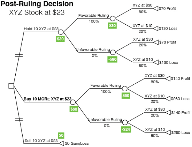
Figure 14.11 Post‐ruling decision tree
There is a difference, though, between simply making the decision to be long and the decision about how long you should be. Let's say you want your expected upside to be twice your expected downside. Initially that required an entry price below $20.30, which is why you had purchased it when it dropped to $20. Now, the decision is whether to hold, double down or sell it all. Again, you decide that you will double down after the ruling if the expected upside is at least 2x the expected downside. If the ratio is below that you'll stick with what you have, and if it's at $30 you'll sell it all. Therefore, given your post‐ruling probabilities, you should double down if the stock is below $23.33.
Note that those parameters can, and should, all be set prior to entering the initial trade. Since those parameters are the decisions as they relate to this investment, no actual decision needs to be made as new information becomes available, only execution of those made in a moment of maximum objectivity.
The Natural Beauty of (Decision) Trees
Table 14.2 shows a decision matrix created to assess the expected returns for a hedge fund manager that an allocator is considering for an investment. In the second column are the returns projected by an analyst for the seven mutually exclusive potential outcomes as he has defined them. The next column contains the probability that each of those scenarios will occur. We know these outcomes are both exhaustive and mutually exclusive because the sum of the probabilities of the seven scenarios totals 100%. As you know, the total expected return is a function of the expected returns for each scenario and their respective probabilities. If the first four columns were all we knew it would be difficult to find a flaw in the analysis. However, the content of column five calls everything that came before it into question. Let's explore why that is and what can be done to avoid this mistake going forward.
Table 14.2 Decision matrix
| Expected Return | Probability | Weighted Expected Return | Reason | |
| Scenario 1 | −5.0% | 3% | −0.2% | 2008 occurs again, xxxx performs better due to high quality focus of portfolio. |
| Scenario 2 | −2.5% | 7% | −0.2% | Market declines 7.5%, xxxx creates no alpha. |
| Scenario 3 | 6.0% | 10% | 0.6% | Market is relatively flat, xxxx creates 6% annualized alpha. |
| Scenario 4 | 8.4% | 20% | 1.7% | Markets hits historical return profile of 8%, xxxx creates 300bps of alpha. |
| Scenario 5 | 13.1% | 40% | 5.2% | xxxx matches historical return profile. |
| Scenario 6 | 24.1% | 15% | 3.6% | xxxx is able to benefit from volatile market and generate material alpha on both sides of the portfolio. |
| Scenario 7 | 33.7% | 5% | 1.7% | US economy outperforms, benefiting small and midcap companies, allowing xxxx to materially outperform broad market strength. |
| Total Expected Return | 12.5% | |||
One factor mentioned in several of the scenario “reasons” comments on the performance of the “markets,” thereby implying that there is a beta component to this fund manager's returns. In other words, there is a correlation between market returns and this fund's returns. Based on the description in Scenario 1, that correlation is thought to be positive. According to this analyst there are three other key variables that contribute to the fund's returns – alpha, market volatility and the US economy.
In order for the probabilities of all seven possible scenarios to add up to 100% they must be mutually exclusive. Scenario 1 is very specific, calling for –35% returns for the Russell 2000 (very negative) over the next 12 months. Scenario 2 calls for a 7.5% decline (slightly negative) in R2K without any alpha generation. Scenario 3 calls for zero return in R2K, but positive alpha. Scenario 4 calls for R2K to rally 8% (slightly positive), plus 300 bps of alpha. The remaining scenarios make no mention of market returns, which means they could occur under any or all market outcomes, including those previously defined. Scenario 5 mentions only the fund's future returns in isolation so we know nothing about any of the variables on which the fund's returns are dependent. Scenario 6 anticipates volatile markets and positive alpha leading to a 24.1% return. Scenario 7 expects a strong economy and market returns, resulting in a 33.7% return for the fund. Even reading through the reasons one at a time, it's difficult to see that there is a problem with the analysis, but there is a flaw, and it's significant.
Table 14.3 shows a summary of the information provided so far.
Table 14.3 Seven scenarios: probability
| Market Returns | Alpha | Market Volatility | US Economy | Fund Returns | |
| Scenario 1 | Very Negative | –5% | |||
| Scenario 2 | Slightly Negative | None | –2.5% | ||
| Scenario 3 | Flat | Positive | 6.0% | ||
| Scenario 4 | Slightly Positive | Positive | 8.4% | ||
| Scenario 5 | 13.1% | ||||
| Scenario 6 | Positive | High | 24.1% | ||
| Scenario 7 | Strong | 33.7% |
Even seeing it in this table format doesn't really help us see the problem. To make it leap off the page, rather than using a matrix, let's review the information one scenario at a time using decision trees (Figure 14.12–14.17).

Figure 14.12 Scenario 1 decision tree
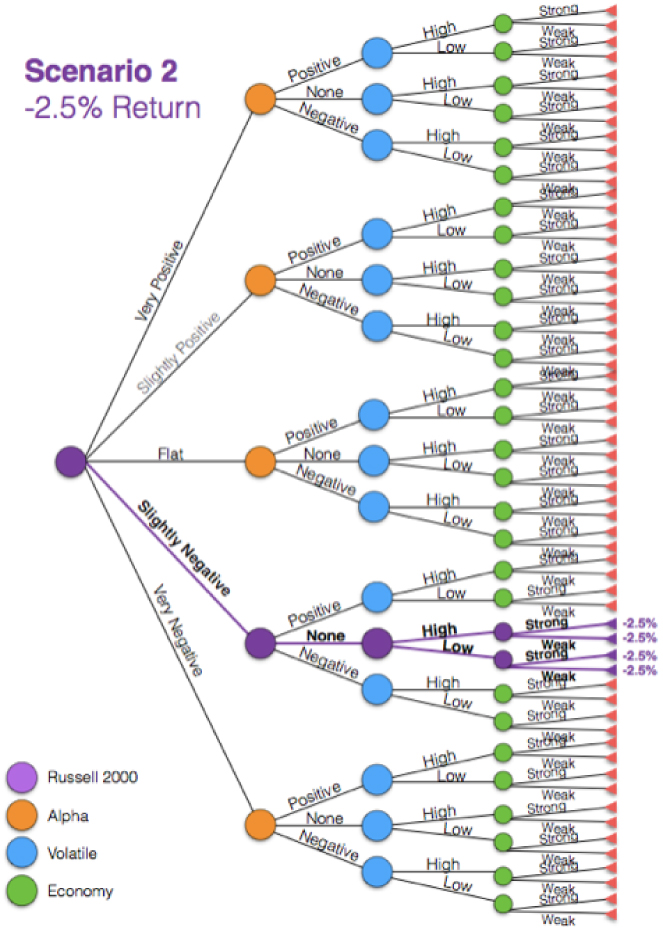
Figure 14.13 Scenario 2 decision tree

Figure 14.14 Scenario 3 decision tree

Figure 14.15 Scenario 4 decision tree
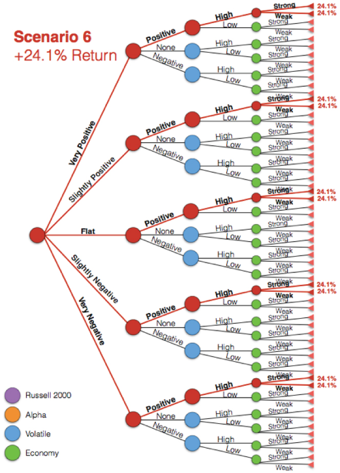
Figure 14.16 Scenario 6 decision tree
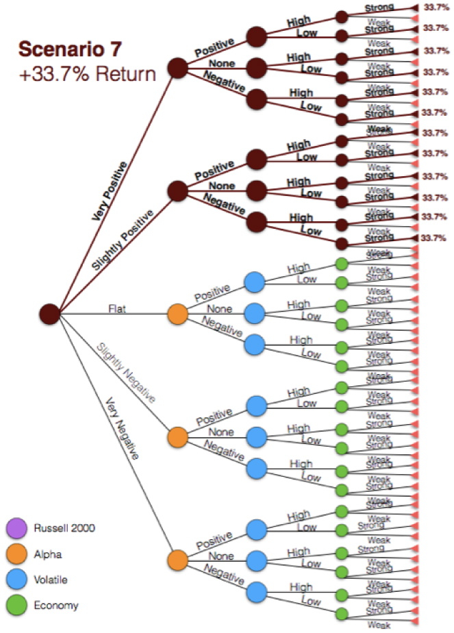
Figure 14.17 Scenario 7 decision tree
If done correctly, every branch should be represented by one, and only one, mutually exclusive scenario. When added together, they will total 100%. As you can see in the Figure 14.18, quite a few branches are part of more than one scenario, and we haven't even included Scenario 5, because it isn't defined according to the variables chosen by the analyst.
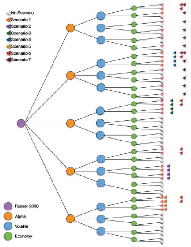
Figure 14.18 Decision tree for Scenarios 1–7
The point I'm attempting to make here is that based upon the way these scenarios have been defined they are neither mutually exclusive nor are they likely exhaustive. That's important, because it means the +12.5% expected return spit out at the end of his analysis is incomplete, incorrect, and essentially useless.
The correct way to carry out such a complex expected return analysis begins by laying out the relevant variables (Figure 14.19). The analyst must then set his expectations for each and every branch segment (Figure 14.20). You'll notice that each choice node (represented by circles) has a set of branches that add up to 100%.
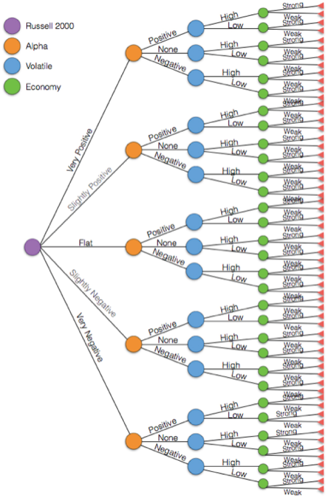
Figure 14.19 Relevant variables only
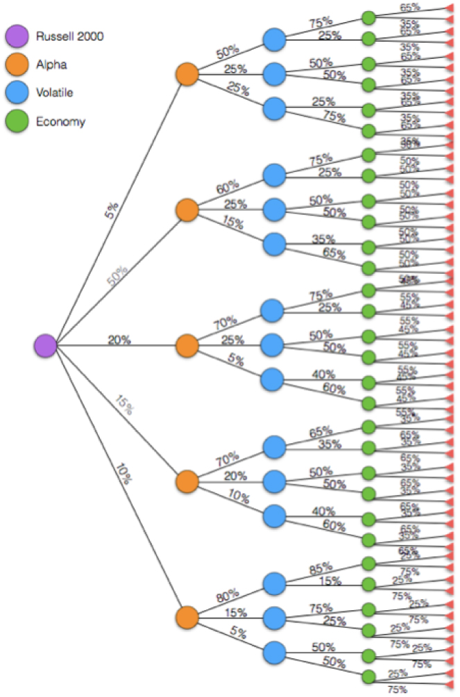
Figure 14.20 Expectations for each branch segment
The only things left to do then are set return expectations for each scenario and multiply each of them by the relevant probability. It requires time, effort, and cognitive strain to produce this analysis which is why so few do it, and so many struggle with trade management decisions during an investment's lifecycle.
The decision tree is not only an excellent tool for unearthing mistakes in an analysis, it may be the most valuable tool available for those looking to shift from a reactive decision making process to a proactive one.
Valuing Liquidity
Let's explore one final situation in which investors could benefit from the use of decision trees. This one helps us to truly appreciate one of the great advantages of liquidity.
Assume you are choosing between a private equity deal (Figure 14.21) in which you are locked in for three years versus an allocation to a global macro hedge fund that allows for monthly liquidity. You've done a significant amount of analysis on the history of returns on your allocation decisions and it turns out that the two funds you are considering for an allocation share the same three year expected return profile as the average investment in your “Moderately Aggressive” risk bucket. Therefore, the decision tree for both investments should look identical, right? Of course, you recognize that there is a tangible benefit to the hedge fund's liquidity terms, but how can you quantify that benefit so that it is appropriately and consistently assessed?
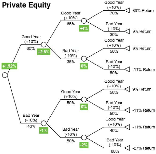
Figure 14.21 Private equity deal
Just because the expected return profiles for both investments are identical doesn't mean that the decision trees will be the same. They will differ for this investor for two reasons. First, she has recognized a trend in the investments she makes. Year 1 returns provide predictive value regarding year 2 returns, and the combo of year 1 plus year 2 returns offers valuable information about the likelihood of profitability in year 3. Although this is true for both the private equity fund and the hedge fund, liquidity terms only allow the investor to capitalize on it in the hedge fund allocation. The ability to potentially act on that new information is the second reason the decisions trees will differ.
Let's look at the decision facing the investor in the hedge fund at the end of a bad 1st year (Figure 14.22). The choice she faces is whether to redeem from the current hedge fund and invest the proceeds in something else or stick with the current hedge fund manager. Based on the investor's data, the rational choice is to redeem and invest elsewhere. (After a good year 1, the rational choice is to stay with the current manager.) The same analysis should be done after a bad year 2 (Figure 14.23). Based on her data, she decides ahead of time that she will redeem and invest elsewhere whenever a hedge fund manager has a bad year. Given that information, we can create the full decision tree, and expected return, for an investment in the hedge fund (Figure 14.24).
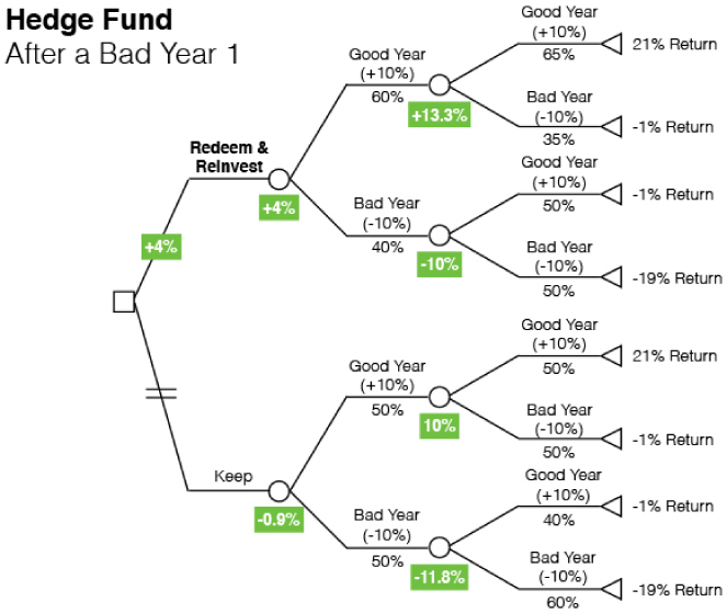
Figure 14.22 Bad year 1

Figure 14.23 Bad year 2

Figure 14.24 Full expected returns in year 1
Turns out the expected return for the hedge fund is +2.6% versus +1.52% for the private equity investment with the only difference being the ability to make an adjustment to the investment as more information becomes available.
(Notice, again, the decision is made ahead of time. Only the execution occurs in the moment the new information becomes available.)
In the first section of this chapter, “What Makes Trading So Difficult,” I made a seemingly controversial claim that your maximum position size should be at the bottom of an upward sloping trend channel while gradually reducing the position until there is nothing left just below the top of it. The alternative is the approach most investors take. Wait until it bounces back up to $20, thereby “confirming” your view, which gives you confidence to size up the position, but at a far less attractive level.
Now I know many of you will argue that you should move the stop‐loss up along the way to reduce the potential maximum downside. And yes, it does reduce the maximum potential downside, allowing you to size up the position, but when you do that, you must also shift the probability of triggering that stop‐loss significantly higher (Figure 14.25). Because in this trade we have binary expectations, meaning that these probabilities are a function of hitting the take‐profit level prior to the stop‐loss level and vice‐versa, if we raise the probability of triggering the stop‐loss, we must also reduce the probability of triggering the take‐profit by a commensurate amount, the combination of which will have a negative impact on your expected return. So, although moving the stop‐loss up will reduce the likelihood of a maximum drawdown, it doesn't make it a more attractive investment, and certainly nowhere near as attractive as it is near the bottom of the range.

Figure 14.25 Shifting stop‐loss higher (left) compared with proper stop‐loss placement (right)
There is a way to make it a more attractive investment opportunity, though. Given that technical support (i.e. the bottom of the range) represents a discrete moment where the odds of spot trading below that point drop disproportionately, moving the stop‐loss to a level just below the support line will have a disproportionate impact on the attractiveness of the trade.
Now let's assume the court ruling came out as you expected. Does it change anything? Do we need to make any adjustments? Absolutely. The expected returns change, even if the maximum potential drawdown doesn't. Table 14.4 reflects the updated expectations. As you can see, your take‐profit should be raised to $26.
Table 14.4 After court ruling
| Stock Price | Expected Return | Prob of Upper Tgt | Rtn at Upper Tgt | Prob of Lower Expec | Rtn at Lower Expec | Max Downside | Notional |
| 30 | −13.33% | 80% | 0.0% | 20% | −66.7% | −1,000,000 | 1,500,000 |
| 29 | −10.00% | 80% | 3.3% | 20% | −63.3% | −1,000,000 | 1,578,947 |
| 28 | −6.67% | 80% | 6.7% | 20% | −60.0% | −1,000,000 | 1,666,667 |
| 27 | −3.33% | 80% | 10.0% | 20% | −56.7% | −1,000,000 | 1,764,706 |
| 26 | 0.00% | 80% | 13.3% | 20% | −53.3% | −1,000,000 | 1,875,000 |
| 25 | 3.33% | 80% | 16.7% | 20% | −50.0% | −1,000,000 | 2,000,000 |
| 24 | 6.67% | 80% | 20.0% | 20% | −46.7% | −1,000,000 | 2,142,857 |
| 23 | 10.00% | 80% | 23.3% | 20% | −43.3% | −1,000,000 | 2,307,692 |
| 22 | 13.33% | 80% | 26.7% | 20% | −40.0% | −1,000,000 | 2,500,000 |
| 21 | 16.67% | 80% | 30.0% | 20% | −36.7% | −1,000,000 | 2,727,273 |
| 20 | 20.00% | 80% | 33.3% | 20% | −33.3% | −1,000,000 | 3,000,000 |
| 19 | 23.33% | 80% | 36.7% | 20% | −30.0% | −1,000,000 | 3,333,333 |
| 18 | 26.67% | 80% | 40.0% | 20% | −26.7% | −1,000,000 | 3,750,000 |
| 17 | 30.00% | 80% | 43.3% | 20% | −23.3% | −1,000,000 | 4,285,714 |
| 16 | 33.33% | 80% | 46.7% | 20% | −20.0% | −1,000,000 | 5,000,000 |
| 15 | 36.67% | 80% | 50.0% | 20% | −16.7% | −1,000,000 | 6,000,000 |
| 14 | 40.00% | 80% | 53.3% | 20% | −13.3% | −1,000,000 | 7,500,000 |
| 13 | 43.33% | 80% | 56.7% | 20% | −10.0% | −1,000,000 | 10,000,000 |
| 12 | 46.67% | 80% | 60.0% | 20% | −6.7% | −1,000,000 | 15,000,000 |
| 11 | 50.00% | 80% | 63.3% | 20% | −3.3% | −1,000,000 | 30,000,000 |
| 10 | 53.33% | 80% | 66.7% | 20% | 0.0% | −1,000,000 | 0 |
As I stated at the beginning I have purposely kept this example simple. However, the approach can be expanded to accommodate all of your expectations no matter how detailed they may be. In order for any of this to work you must properly define all of your expectations ahead of time. I believe you will be impressed with the benefits of shifting from the standard reactive approach to decision making to a proactive one. Yes, it requires a significant amount of work and cognitive strain to be invested up front, but it dramatically reduces the number of decisions that need to be made throughout the life of the trade. Most importantly, it reduces the number of decisions that will need to be made under emotional distress and time constraints, thereby improving the odds of more rational choices being made throughout. In the end, that is the key to better returns.