
Chapter 6
ASSET AND LIABILITY MANAGEMENT II
In our second ALM chapter, we delve deeper – or more accurately wider – into the topic. The art of asset and liability management is essentially one of risk management and capital management, and although day-to-day activities are run at the desk level, overall direction is given at the highest level of a banking institution. Risk exposures in a banking environment are multi-dimensional; as we have seen, they encompass interest rate risk, liquidity risk, credit risk and operational risk. Interest rate risk is one type of market risk. Risks associated with moves in interest rates and levels of liquidity1 are those that result in adverse fluctuations in earnings levels due to changes in market rates and bank funding costs. By definition, banks’ earnings levels are highly sensitive to moves in interest rates and the cost of funds in the wholesale market. Asset and liability management covers the set of techniques used to manage interest rate and liquidity risks; it also deals with the structure of the bank’s balance sheet, which is heavily influenced by funding and regulatory constraints and profitability targets.
In this chapter we review the concept of balance sheet management, the role of the ALM desk, liquidity risk and maturity gap risk. We also review a basic gap report. The increasing use of securitization and the responsibility of the ALM desk in enhancing the return on assets on the balance sheet is also introduced. For readers who are interested in developing their knowledge further, we list a selection of articles and publications in the Bibliography at the end of the chapter.
INTRODUCTION
For newcomers to the subject, an excellent introduction to the primary activity of banking is contained in an article in The Economist entitled ‘The business of banking’.2 Those who are complete beginners may wish to refer to this article. In this section we provide an overview of the main business of banking before considering the subject of ALM.
One of the major areas of decision-making in a bank involves the maturity of assets and liabilities. Typically, longer term interest rates are higher than shorter term rates; that is, it is common for the yield curve in the short term (say 0-to-3-year range) to be positively sloping. To take advantage of this banks usually raise a large proportion of their funds from the short-dated end of the yield curve and lend out these funds for longer maturities at higher rates. The spread between borrowing and lending rates is in principle the bank’s profit. The obvious risk from such a strategy is that the level of short-term rates rises during the term of the loan, so that when the loan is refinanced the bank makes a lower profit or a net loss. Managing this risk exposure is the key function of an ALM desk. As well as managing the interest rate risk itself, banks also match assets with liabilities – thus locking in a profit – and diversify their loan book, to reduce exposure to one sector of the economy.
Another risk factor is liquidity. From a banking and Treasury point of view the term liquidity means funding liquidity, or the ‘nearness’ of money. The most liquid asset is cash money. Banks bear several interrelated liquidity risks, including the risk of being unable to pay depositors on demand, an inability to raise funds in the market at reasonable rates and an insufficient level of funds available with which to make loans. Banks keep only a small portion of their assets in the form of cash, because this earns no return for them. In fact, once they have met the minimum cash level requirement, which is something set down by international regulation (reviewed in the previous chapter), they will hold assets in the form of other instruments. Therefore, the ability to meet deposit withdrawals depends on a bank’s ability to raise funds in the market. The market and the public’s perception of a bank’s financial position heavily influences liquidity. If this view is very negative, the bank may be unable to raise funds and consequently be unable to meet withdrawals or loan demand. Thus, liquidity management is running a bank in a way that maintains confidence in its financial position. The assets of the banks that are held in near-cash instruments, such as Treasury bills and clearing bank CDs, must be managed with liquidity considerations in mind. The asset book on which these instruments are held is sometimes called the liquidity book.
Basic concepts
In the era of stable interest rates that preceded the breakdown of the Bretton Woods agreement, ALM was a more straightforward process, constrained by regulatory restrictions and the saving and borrowing pattern of bank customers.3 The introduction of the negotiable certificate of deposit by Citibank in the 1960s enabled banks to diversify both their investment and funding sources. With this there developed the concept of interest margin, which is the spread between the interest earned on assets and that paid on liabilities. This led to the concept of interest gap and management of the gap, which is the cornerstone of modern-day ALM. The increasing volatility of interest rates, and the rise in absolute levels of rates themselves, made gap management a vital part of running the banking book. This development meant that banks could no longer rely permanently on the traditional approach of borrowing short (funding short) to lend long, as a rise in the level of short-term rates would result in funding losses. The introduction of derivative instruments such as FRAs and swaps in the early 1980s removed the previous uncertainty and allowed banks to continue the traditional approach while hedging against medium-term uncertainty.
Foundations of ALM
The general term asset and liability management entered common usage from the mid-1970s onwards. Under a changing-interest-rate environment, it became imperative for banks to manage both assets and liabilities simultaneously, in order to minimize interest rate and liquidity risk and maximize interest income. ALM is a key component of any financial institution’s overall operating strategy. As described in previous texts (Marshall and Bansal, 1992, pp. 498–501) ALM is defined in terms of four key concepts, which are described below.
The first is liquidity, which in an ALM context does not refer to the ease with which an asset can be bought or sold in the secondary market, but the ease with which assets can be converted into cash.4 A banking book is required by the regulatory authorities to hold a specified minimum share of its assets in the form of very liquid instruments. Liquidity is very important to any institution that accepts deposits because of the need to meet customer demand for instant access funds. In terms of a banking book the most liquid assets are overnight funds, while the least liquid are medium-term bonds. Short-term assets such as T-bills and CDs are also considered to be very liquid.
The second key concept is the money market term structure of interest rates. The shape of the yield curve at any one time, and expectations as to its shape in the short term and medium term, significantly impact the ALM strategy employed by a bank. Market risk in the form of interest rate sensitivity, in the form of the present value sensitivity of specific instruments to changes in the level of interest rates, and in the form of the sensitivity of floating rate assets and liabilities to changes in rates are all significant. Another key factor is the maturity profile of the book. The maturities of assets and liabilities can be matched or unmatched; although the latter is more common the former is not uncommon depending on the specific strategies that are being employed. Matched assets and liabilities lock in return in the form of the spread between the funding rate and the return on assets. The maturity profile, the absence of a locked-in spread and the yield curve combine to determine the total interest rate risk of the banking book.
The fourth key concept is default risk: the risk exposure that borrowers will default on interest or principal payments that are due to the banking institution.
These issues are placed in context in the simple hypothetical situation described in Box 6.1.
Box 6.1 ALM considerations
Assume that a bank wants to access the markets for 3-month and 6-month funds, whether for funding or investment purposes. The rates for these terms are shown in Table 6.1. Assume there are no bid–offer spreads. The ALM manager also expects the 3-month Libor rate in 3 months’ time to be 5.10%. The bank can usually fund its book at Libor while it is able to lend at Libor plus 1%.
Table 6.1 Hypothetical money market rates
| Term | Libor | Bank rate |
| 90-day | 5.50% | 6.50% |
| 180-day | 5.75% | 6.75% |
| Expected 90-day rate in 90 days' time | 5.10% | 6.10% |
| 3v6 FRA | 6.60% |
The bank could adopt any of the following strategies or a combination of them:
- Borrow 3-month funds at 5.50% and lend them for a 3-month period at 6.50%. This locks in a return of 1% for a 3-month period.
- Borrow 6-month funds at 5.75% and lend them for a 6-month period at 6.75%; again this earns a locked-in spread of 1%.
- Borrow 3-month funds at 5.50% and lend them for a 6-month period at 6.75%. This approach would require the bank to refund the loan in 3 months’ time, which it expects to be able to do at 5.10%. This approach locks in a return of 1.25% in the first 3-month period and an expected return of 1.65% in the second 3-month period. The risk of this tactic is that the 3-month rate in 3 months’ time does not fall as expected by the ALM manager, reducing profits and possibly leading to loss.
- Borrow 6-month funds at 5.75% and lend them for a 3-month period at 6.50%. After this period, lend the funds for a 3-month or 6-month period. This strategy does not tally with the ALM manager’s view, however, who expects a fall in rates and so should not wish to be long of funds in 3 months’ time.
- Borrow 3-month funds at 5.50% and again lend them for a 6-month period at 6.75%. To hedge the gap risk, the ALM manager simultaneously buys a 3v6 FRA to lock in the 3-month rate in 3 months’ time. The first period spread of 1.25% is guaranteed, but the FRA guarantees only a spread of 15 basis points in the second period. This is the cost of the hedge (and also suggests that the market does not agree with the ALM manager’s assessment of where rates will be 3 months from now!); the price the bank must pay for reducing uncertainty is lower spread return. Alternatively, the bank could lend for a 6-month period, funding initially for a 3-month period, and buy an interest rate cap with a ceiling rate of 6.60% that is pegged to Libor, the rate at which the bank can actually fund its book.
Although simplistic, these scenarios serve to illustrate what is possible; indeed, there are many other strategies that could be adopted. The approaches described in the last option show how derivative instruments can actively be used to manage the banking book and the cost associated with employing them.
Liquidity and gap management
We have noted that the simplest approach to ALM is to match assets with liabilities. For a number of reasons – including the need to meet client demand and to maximize return on capital – this is not practical and banks must adopt more active ALM strategies. One of the most important of these is the role of the gap and gap management. This term describes the practice of varying the asset and liability gap in response to expectations about the future course of interest rates and the shape of the yield curve. Simply put, this means increasing the gap when interest rates are expected to rise and decreasing it when rates are expected to decline. The gap here is the difference between floating rate assets and liabilities, but gap management must also be pursued when one of these elements is fixed rate.
Such a discipline is of course as much an art as a science. Gap management assumes that the ALM manager is proved to be correct in his prediction of the future direction of rates and the yield curve.5 Views that turn out to be incorrect can lead to unexpected widening or narrowing of the gap spread and losses. The ALM manager must choose the level of tradeoff between risk and return.
Gap management also assumes that the profile of the banking book can be altered with relative ease. This was not always the case, and even today may still present problems, although evaluation of a liquid market in off-balance-sheet interest rate derivatives has eased this problem somewhat. Historically, it has always been difficult to change the structure of the book, as many loans cannot be liquidated instantly and fixed rate assets and liabilities cannot be changed to floating rate ones. Client relationships must also be observed and maintained – a key banking issue. For this reason it is much more common for ALM managers to use off-balance-sheet products when dynamically managing the book. For example, FRAs can be used to hedge gap exposure, while interest rate swaps are used to alter an interest basis from fixed to floating – or vice versa. The last strategy presented in Box 6.1 presented, albeit simplistically, the use that could be made of derivatives. The widespread use of derivatives has enhanced the opportunities available to ALM managers, as well as the flexibility with which the banking book can be managed, but it has also contributed to an increase in competition and a reduction in margins and bid–offer spreads.
Interest rate risk and source
Interest rate risk
Put simply, interest rate risk is defined as the potential impact – adverse or otherwise – on the net asset value of a financial institution’s balance sheet and earnings resulting from a change in interest rates. Risk exposure exists whenever there is a maturity date mismatch between assets and liabilities, or between principal and interest cashflows. Interest rate risk is not necessarily a negative thing; for instance, changes in interest rates that increase the net asset value of a banking institution would be regarded as positive. For this reason, active ALM seeks to position a banking book to gain from changes in rates. The Bank for International Settlements splits interest rate risk into two elements: investment risk and income risk. The first risk type is the term for potential risk exposure arising from changes in the market value of fixed-interest-rate cash instruments and off-balance-sheet instruments, and is also known as price risk. Investment risk is perhaps best exemplified by the change in value of a plain vanilla bond following a change in interest rates, and from Chapter 2 we know that there is an inverse relationship between changes in rates and the value of such bonds (see Example 2.2). Income risk is the risk of loss of income when there is a non-synchronous change in deposit and funding rates – it is this risk that is known as gap risk.
ALM covering the formulation of interest rate risk policy is usually the responsibility of what is known as the asset–liability committee (ALCO), which is made up of senior management personnel including the finance director and the heads of Treasury and risk management. The ALCO sets bank policy for balance sheet management and the likely impact on revenue of various scenarios that it considers may occur. The number of people who sit on the ALCO will depend on the complexity of the balance sheet and products traded, as well as the amount of management information available on individual products and desks.
The process employed by the ALCO for ALM will vary according to the particular internal arrangement of the institution. A common procedure involves a monthly presentation to the ALCO of the impact of different interest rate scenarios on the balance sheet. This presentation may include
- Analysis of the difference between actual net interest income (NII) for the previous month and the amount that was forecast at the previous ALCO meeting. This is usually presented as a gap report, broken by maturity buckets and individual products.
- The result of discussion with business unit heads on the basis of the assumptions used in calculating forecasts and the impact of interest rate changes; scenario analysis usually assumes an unchanging book position between now and 1 month later, which is essentially unrealistic.
- A number of interest rate scenarios, based on assumptions of (a) what is expected to happen to the shape and level of the yield curve, and (b) what could conceivably happen to it – for example, extreme scenarios. Essentially, this exercise produces a value for forecast NII due to changes in interest rates.
- Update of the latest actual revenue numbers.
Specific new or one-off topics may be introduced at the ALCO as circumstances dictate; for example, presentation of an approval process for the introduction of a new product.
Sources of interest rate risk
Assets on the balance sheet are affected by absolute changes in interest rates as well as increases in the volatility of interest rates. For instance, fixed rate assets will fall in value in the event of a rise in rates, while funding costs will rise. This decreases the margins available. We noted that the way to remove this risk was to lock in assets with matching liabilities; however, this is not only not always possible, but also sometimes undesirable, as it prevents the ALM manager from taking a view on the yield curve. In a falling interest rate environment, deposit-taking institutions may experience a decline in available funds, requiring new funding sources that may be accessed at less favourable terms. Liabilities are also impacted by a changing interest rate environment.
There are five primary sources of interest rate risk inherent in an ALM book:
- Gap risk is the risk that revenue and earnings decline as a result of changes in interest rates, due to differences between the maturity profiles of assets, liabilities and off-balance-sheet instruments. Another term for gap risk is mismatch risk. An institution with gap risk is exposed to changes in the level of the yield curve – so-called parallel shift – or change in the shape of the yield curve – so-called pivotal shift. Gap risk is measured in terms of short-term or long-term risk, which is a function of the impact of rate changes on earnings for a short or long period. Therefore, the maturity profile of the book and the time to maturity of instruments held on the book will influence whether the bank is exposed to short-term or long-term gap risk.
- Yield curve risk is the risk that non-parallel or pivotal shifts in the yield curve cause a reduction in NII. The ALM manager will change the structure of the book to take into account his views on the yield curve. For example, a book with a combination of short-term and long-term asset or liability maturity structures6 is at risk from yield curve inversion, sometimes known as a twist in the curve.
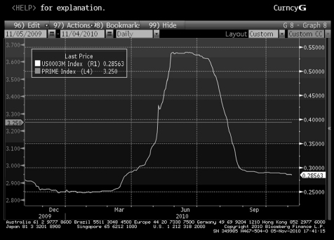
- Basis risk arises from the fact that assets are often priced off one interest rate, while funding is priced off another interest rate. Taken one step further, hedge instruments are often linked to a different interest rate from that of the product they are hedging. In the US market the best example of basis risk is the difference between the Prime rate and Libor. Term loans in the US are often set at Prime, or a relationship to Prime, while bank funding is usually based on the Eurodollar market and linked to Libor. However, the Prime rate is what is known as an ‘administered’ rate and does not change on a daily basis – unlike Libor. While changes in the two rates are positively correlated, they do not change by the same amount, which means that the spread between them changes regularly. This results in spread earning on a loan product changing over time. Figure 6.1 illustrates the change in spread during 2009–2010.
- Another risk for deposit-taking institutions such as clearing banks is runoff risk, associated with the non-interest-bearing liabilities (NIBLs) of such banks. The level of interest rates at any one time represents an opportunity cost to depositors who have funds in such facilities. However, in a rising-interest-rate environment, this opportunity cost rises and depositors will withdraw these funds, available at immediate notice, resulting in an outflow of funds from the bank. The funds may be taken out of the banking system completely; for example, for investment in the stock market. This risk is significant and therefore sufficient funds must be maintained at short notice, which is an opportunity cost for the bank itself.
- Many banking products entitle the customer to terminate contractual arrangements ahead of the stated maturity term; this is sometimes referred to as option risk. This is another significant risk as products – such as CDs, cheque account balances and demand deposits – can be withdrawn or liquidated at no notice, which is a risk to the level of NII should the option inherent in the products be exercised.
Figure 6.1 Change in spread between Prime rate and USD 3-month Libor 20092010.
© Bloomberg L.P. Used with permission. Visit www.bloomberg.com.
Gap and net interest income
We noted earlier that gap is a measure of the difference between the interest rate sensitivity of assets and liabilities that revalue at a particular date, expressed as a cash value. Put simply it is
(6.1) ![]()
where and are interest-rate-sensitive assets and interest-rate-sensitive liabilities. Where the banking book is described as being positively gapped, and when the book is said to be negatively gapped. The change in NII is given by
(6.2) ![]()
where is the relevant interest rate used for valuation. The NII of a bank that is positively gapped will increase as interest rates rise and decrease as rates decline. This describes a banking book that is asset sensitive; the opposite, when a book is negatively gapped, is known as liability sensitive. The NII of a negatively gapped book will increase when interest rates decline. The value of a book with zero gap is immune to changes in the level of interest rates. The shape of the banking book at any one time is a function of customer demand, the Treasury manager’s operating strategy, as well as a view of future interest rates.
Gap analysis is used to measure the difference between interest-rate-sensitive assets and liabilities over specified time periods. Another term for this analysis is periodic gap, and the common expression for each time period is a maturity bucket. For a commercial bank typical maturity buckets are:
0–3 months;
3–12 months;
1–5 years;
5 years.
Another common approach is to group assets and liabilities by the buckets or grid points of the Riskmetrics value-at-risk methodology. Moreover, any combination of time periods may be used. For instance, certain US commercial banks place assets, liabilities and off-balance-sheet items in terms of known maturities, judgemental maturities and market-driven maturities:
- known maturities are fixed rate loans and CDs;
- judgemental maturities are passbook savings accounts, demand deposits, credit cards and non-performing loans;
- market-driven maturities are option-based instruments such as mortgages and other interest-rate-sensitive assets.
The other key measure is cumulative gap, defined as the sum of individual gaps up to 1-year maturity. Banks traditionally use cumulative gap to estimate the impact of a change in interest rates on NII.
Assumptions of gap analysis
A number of assumptions are made when using gap analysis, but they may not reflect reality in practice. These include
- The key assumption that interest rate changes manifest themselves as a parallel shift in the yield curve; in practice, changes do not occur as a parallel shift, giving rise to basis risk between short-term and long-term assets.
- The expectation that contractual repayment schedules are met; if there is a fall in interest rates, prepayments of loans by borrowers who wish to refinance their loans at lower rates will have an impact on NII. Certain assets and liabilities have option features that are exercised as interest rates change, such as letters of credit and variable rate deposits; early repayment will impact a bank’s cashflow.
- The expectation that repricing of assets and liabilities takes place at the midpoint of the time bucket.
- The expectation that all loan payments will occur on schedule; in practice, certain borrowers will repay the loan earlier.
Recognized weaknesses of the gap approach include
- no incorporation of future growth, or changes in the asset/liability mix;
- no consideration of the time value of money;
- arbitrary setting of time periods.
Limitations notwithstanding, gap analysis is used extensively. Gup and Brooks (1993, p. 59) give the following reasons for the continued popularity of gap analysis:
- it was the first approach introduced to handle interest rate risk – it provides reasonable accuracy;
- the data required to perform the analysis have already been compiled for the purposes of regulatory reporting;
- gaps can be calculated using simple spreadsheet software;
- it is easier (and cheaper) to implement than more sophisticated techniques;
- it is straightforward to demonstrate and explain to senior management and shareholders.
Although there are more sophisticated methods available, gap analysis remains in widespread use.
THE BANKING BOOK
Traditionally, ALM has been concerned with the banking book. The conventional techniques of ALM were developed for application to a bank’s banking book – that is, its lending and deposit-taking transactions. The core banking activity will generate either an excess of funds (when the receipt of deposits outweighs the volume of lending the bank has undertaken) or a shortage of funds (when the reverse occurs). This mismatch is balanced via financial transactions in the wholesale market. The banking book generates both interest rate and liquidity risks, which are then monitored and managed by the ALM desk. Interest rate risk is the risk that the bank suffers losses due to adverse movements in market interest rates. Liquidity risk is the risk that the bank cannot generate sufficient funds when required; the most extreme version of this is when there is a run on the bank and the bank cannot raise the funds required when depositors withdraw their cash.
Note that the asset side of the banking book – that is, the loan portfolio – also generates credit risk.
The ALM desk will be concerned with risk management that focuses on the quantitative management of liquidity and interest rate risks inherent in a banking book. The major areas of ALM include
- Measurement and monitoring of liquidity and interest rate risk. This includes setting up targets for earnings and the volume of transactions, as well as setting up and monitoring interest rate risk limits.
- Funding and control of any constraints on the balance sheet. This includes liquidity constraints and debt policy as well as the capital adequacy ratio and solvency.
- Hedging of liquidity and interest-rate risk.
THE ALM DESK
The ALM desk or unit is a specialized business unit that fulfils a range of functions. Its precise remit is a function of the type of activities of the financial institution it is a part of. Let us consider the main types of activities that are carried out.
If an ALM unit has a profit target of zero, it will act as a cost centre with a responsibility to minimize operating costs. This would be consistent with a strategy that emphasizes commercial banking as the core business of the firm, and where ALM policy is concerned purely with hedging interest rate and liquidity risk.
The next stage of development is where the ALM unit is responsible for minimizing the cost of funding. This would allow the unit to maintain an element of exposure to interest rate risk, depending on the view that was held as to the future level of interest rates. As we noted above, the core banking activity generates either an excess or shortage of funds. To hedge away all the excess or shortage, while removing interest rate exposure, has an opportunity cost associated with it since it eliminates any potential gain that might arise from movements in market rates. Of course, without a complete hedge, there is exposure to interest rate risk. The ALM desk is responsible for monitoring and managing this risk and, of course, is credited with any cost savings in the cost of funds that arise from exposure. Savings may be measured as the difference between the funding costs of a full hedging policy and the actual policy that the ALM desk adopts. Under this policy, interest rate risk limits are set which the ALM desk ensures the bank’s operations do not breach.
The final stage of development is to turn the ALM unit into a profit centre, with responsibility for optimizing the funding policy within specified limits. The limits may be set as gap limits, value-at-risk limits or by another measure – such as the level of earnings volatility. Under this scenario the ALM desk is responsible for managing all financial risk.
The final development of the ALM function has resulted in it taking on a more active role. The previous paragraphs described the three stages of development that ALM has undergone, although all three versions are part of the ‘traditional’ approach. Practitioners are now beginning to think of ALM as extending beyond the risk management field and being responsible for adding value to the net worth of the bank, through proactive positioning of the book and, hence, the balance sheet. That is, in addition to the traditional function of managing liquidity risk and interest rate risk, ALM should be concerned with managing the regulatory capital of the bank and with actively positioning the balance sheet to maximize profit. The latest developments mean that there are now financial institutions that run a much more sophisticated ALM operation than that associated with a traditional banking book.
Let us review the traditional and developed elements of an ALM function.
Traditional ALM
Generally, in the past a bank’s ALM function has been concerned with managing the risk associated with the banking book. This does not mean that this function is now obsolete, rather that additional functions have now been added to the ALM role. There are a large number of financial institutions that adopt the traditional approach; indeed, the nature of their operations would not lend themselves to anything more. We can summarize the role of the traditional ALM desk as follows:
- Interest rate risk management. This is the interest rate risk arising from operation of the banking book. It includes net interest income sensitivity analysis – typified by maturity gap and duration gap analysis – and sensitivity of the book to parallel changes in the yield curve. The ALM desk will monitor the exposure and position the book in accordance with its limits as well as its market view. Smaller banks, or subsidiaries of banks that are based overseas, often run no interest rate risk – that is, there is no short gap in their book. Apart from this, the ALM desk is responsible for hedging interest rate risk or positioning the book in accordance with its view.
- Liquidity and funding management. There are regulatory requirements that dictate the proportion of banking assets that must be held as short-term instruments. The liquidity book in a bank is responsible for running the portfolio of short-term instruments. The exact makeup of the book is, however, the responsibility of the ALM desk and will be a function of the desk’s view of market interest rates, as well as its opinion on the relative value of one asset over another. For example, it may decide to move some assets into short-dated government bonds, in excess of what it normally holds, at the expense of high-quality CDs, or vice versa.
- Reporting on hedging of risks. The ALM fulfils a senior management information function by regularly reporting on the extent of the bank’s risk exposure. This may be in the form of a weekly hardcopy report or via some other medium.
- Setting up risk limits. The ALM unit will set limits, implement them and enforce them, although it is common for an independent ‘middle office’ risk function to monitor compliance with limits.
- Capital requirement reporting. This function involves the compilation of reports on capital usage and position limits as a percentage of capital allowed, as well as reporting to regulatory authorities.
All financial institutions carry out these activities.
Example 6.1 Gap analysis
Maturity gap analysis measures the cash difference or gap between the absolute values of assets and liabilities that are sensitive to movements in interest rates. Therefore, the analysis measures the relative interest rate sensitivities of assets and liabilities, and thus determines the risk profile of the bank with respect to changes in rates. The gap ratio is given as:
![]()
It measures whether there are more interest-rate-sensitive assets than liabilities. A gap ratio higher than 1, for example, indicates that a rise in interest rates will increase the net present value of the book, thus raising the return on assets at a rate higher than the rise in the cost of funding. This also results in a higher income spread.
A gap ratio lower than 1 indicates a rising funding cost. Duration gap analysis measures impact on the net worth of the bank due to changes in interest rates by focusing on changes in the market value of either assets or liabilities. This is because the duration gap measures the percentage change in the market value of a single security for a 1% change in the underlying yield of the security (strictly speaking, this is modified duration but the term for the original ‘duration’ is now almost universally used to refer to modified duration). The duration gap is defined as:
![]()
where is the percentage of assets funded by liabilities. Hence, the duration gap measures the effects of change on the net worth of the bank. A higher duration gap indicates higher interest rate exposure. As the duration gap only measures the effects of a linear change in interest rate – that is, a parallel shift in yield curve change – banks with portfolios that include a significant amount of instruments with elements of optionality (such as callable bonds, asset-backed securities and convertibles) also use the convexity measure of risk exposure to adjust for inaccuracies that arise in the duration gap over large yield changes.
DEVELOPMENTS IN ALM
An increasing number of financial institutions have been enhancing their risk management function by adding to the responsibilities of the ALM function. These have included enhancing the role of the head of Treasury and the ALCO – by using such other risk exposure measures as option-adjusted spread and value-at-risk (VaR) – and integrating traditional interest rate risk management with credit risk and operational risk. The increasing use of credit derivatives has facilitated this integrated approach to risk management.
Additional roles played by the ALM desk may include
- using the VaR tool to assess risk exposure;
- integrating market risk and credit risk;
- using new risk-adjusted measures of return;
- optimizing portfolio return;
- proactively managing the balance sheet – this includes giving direction on the securitization of assets (removing them from the balance sheet), hedging credit exposure using credit derivatives and actively enhancing returns from the liquidity book, such as entering into stock lending and repo.
An enhanced ALM function will by definition expand the role of the Treasury function and the ALCO. This may see the Treasury function becoming active ‘portfolio managers’ of the bank’s book. The ALCO – traditionally composed of risk managers from across the bank as well as the senior member of the ALM desk or liquidity desk – is responsible for assisting the head of Treasury and the finance director in the risk management process. In order to fulfil the new enhanced function the treasurer will require a more strategic approach to his function, as many of the decisions about running the bank’s entire portfolio will be closely connected with the overall direction that the bank wishes to take – these are board-level decisions.
LIQUIDITY AND INTEREST RATE RISK
The liquidity gap
Liquidity risk arises because a bank’s portfolio consists of assets and liabilities with different sizes and maturities. When assets exceed the resources from operations, a funding gap will exist which needs to be sourced in the wholesale market. When the opposite occurs, excess resources must be invested in the market. The difference between assets and liabilities is called the liquidity gap. For example, if a bank has long-term commitments that have arisen from its dealings – and its resources are exceeded by these commitments and have a shorter maturity – there is both an immediate and a future deficit. The liquidity risk for the bank is that there are not enough resources or funds available in the market to balance the assets at any time.
Liquidity management has several objectives; possibly the most important is to ensure that deficits can be funded under all foreseen circumstances and without incurring prohibitive costs. In addition, there are regulatory requirements that force a bank to operate certain limits; these requirements state that short-term assets must be in excess of short-run liabilities in order to provide a safety net of highly liquid assets. Liquidity management is also concerned with funding deficits and investing surpluses, with managing and growing the balance sheet and with ensuring that the bank operates within regulatory and in-house limits. In this section we review the main issues concerned with liquidity and interest rate risk.
The liquidity gap is the difference at all future dates between the assets and liabilities of the banking portfolio. Gaps generate liquidity risk. When liabilities exceed assets, there is an excess of funds. An excess does not of course generate liquidity risk, but it does generate interest rate risk, because the present value of the book is sensitive to changes in market rates. When assets exceed liabilities, there is a funding deficit and the bank has long-term commitments that are not currently funded by existing operations. The liquidity risk is that the bank requires funds at a future date to match the assets. The bank is able to remove any liquidity risk by locking in maturities, but there is of course a cost involved as it will be dealing at longer maturities.7
Gap risk and limits
Liquidity gaps are measured by taking the difference between the outstanding balances of assets and liabilities over time. At any point a positive gap between assets and liabilities is equivalent to a deficit, and this is measured as a cash amount. Marginal gap is the difference between changes in assets and liabilities over a given period. A positive marginal gap means that variation in the value of assets exceeds variation in the value of liabilities. As new assets and liabilities are added over time – as part of the ordinary course of business – the gap profile changes.
The gap profile is tabulated or charted (or both) during and at the end of each day as a primary measure of risk. For illustrative purposes, a tabulated gap report is shown in Table 6.2; this is an actual example from a UK banking institution. It shows assets and liabilities grouped into maturity buckets and the net position for each bucket. It is a snapshot today of the exposure – and hence funding requirement – of the bank for future maturity periods.
Table 6.2 Example gap profile
Table 6.2 is very much a summary figure, because the maturity gaps are very wide. For risk management purposes the buckets would be much narrower; for instance, the period between 0 and 12 months might be split into 12 different maturity buckets. An example of a more detailed gap report is shown in Figure 6.2, which is from another UK banking institution. Note that the overall net position is zero, because this is a balance sheet and therefore, not surprisingly, it balances. However, along the maturity buckets or grid points there are net positions which are the gaps that need to be managed. A full gap report is shown at Table 6.3.
Figure 6.2 Gap limit report.
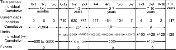
Table 6.3 Detailed gap profile.

Limits on a banking book can be set in terms of gap limits. For example, a bank may set a 6-month gap limit of 10 million. The net position of assets and maturities expiring in 6 months’ time would not then exceed 10 million. An example of a gap limit report is shown at Figure 6.2, with actual net gap positions shown against the gap limits for each maturity. Again this is an actual limit report from a UK banking institution.
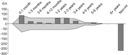
The maturity gap can be charted to provide an illustration of net exposure. An example is shown in Figure 6.3, which is from yet another UK banking institution. In some firms’ reports both assets and liabilities are shown for each maturity point, but in our example only the net position is shown. This net position is the gap exposure for that maturity point. A second example, used by the overseas subsidiary of a middle eastern commercial bank, which has no funding lines in the interbank market and so does not run short positions, is shown at Figure 6.4, while the gap report for a UK high-street bank is shown in Figure 6.5. Note the large short gap under the maturity labelled ‘non-int’; this stands for non-interest-bearing liabilities and represents the balance of current accounts (cheque or ‘checking’ accounts) which are funds that attract no interest and are in theory very short-dated (because they are demand deposits and may be called at instant notice).
Figure 6.3 Gap maturity profile in graphical form.

Figure 6.4 Gap maturity profile of a bank where short funding is not allowed.
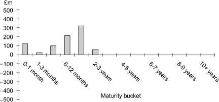
Figure 6.5 Gap maturity profile of a UK high-street bank.
Gaps represent the cumulative funding required at all dates. Cumulative funding is not necessarily identical to the new funding required at each period, because the debt issued in previous periods is not necessarily amortized at subsequent periods. The new funding between, for example, Months 3 and 4 is not the accumulated deficit between Months 2 and 4 because the debt contracted at Month 3 is not necessarily amortized at Month 4. Marginal gaps may be identified as the new funding required or the new excess funds of the period that should be invested in the market. Note that all the reports are snapshots at a fixed point in time and the picture is, of course, continuously moving. In practice, the liquidity position of a bank cannot be characterized by one gap at any given date; the entire gap profile must be used to gauge the extent of the book’s profile.
The liquidity book may decide to match its assets with its liabilities. This is known as cash matching and occurs when the time profiles of assets and liabilities are identical. By following such a course the bank can lock in the spread between its funding rate and the rate at which it lends cash, and run a guaranteed profit. Under cash matching the liquidity gaps will be zero. Matching the profile of both legs of the book is done at the overall level; that is, cash matching does not mean that deposits should always match loans. This would be difficult as both result from customer demand, although an individual purchase of, say, a CD can be matched with an identical loan. Nevertheless, the bank can elect to match assets and liabilities once the net position is known, and keep the book matched at all times. However, it is highly unusual for a bank to adopt a cash-matching strategy.
Liquidity management
The continuous process of raising new funds or investing surplus funds is known as liquidity management. If we consider that the gap today is funded – thus balancing assets and liabilities and squaring off the book – the next day a new deficit or surplus is generated which also has to be funded. The liquidity management decision must cover the amount required to bridge the gap that exists the following day and to position the book across future dates in line with the bank’s view on interest rates. Usually, in order to ascertain the maturity structure of debt a target profile of resources is defined. This may be done in several ways. If the objective of ALM is to replicate the asset profile with resources, the new funding should contribute to bringing the resources profile closer to that of the assets; that is, more of a matched book looking forward. This is the lowest risk option. Another target profile may be imposed on the bank by liquidity constraints. This may arise if, for example, the bank has a limit on borrowing lines in the market such that it could not raise a certain amount each week or month. For instance, if the maximum that could be raised in one week by a bank is 10 million, the maximum period liquidity gap is constrained by that limit. The ALM desk will manage the book in line with the target profile that has been adopted, which requires it to try to reach the required profile over a given time horizon.
Managing the liquidity of the banking book is a dynamic process, as loans and deposits are known at any given point, but new business will be taking place continuously and the profile of the book looking forward must be constantly rebalanced to keep it within the target profile. There are several factors that influence this dynamic process, the most important of which are reviewed below.
Demand deposits
Deposits placed on demand at the bank – such as current accounts (known in the US as ‘checking accounts’) – have no stated maturity and are available on demand at the bank. Technically, they are referred to as ‘non-interest-bearing liabilities’ because the bank pays no or very low rates of interest on them, so they are effectively free funds. The balance of these funds can increase or decrease throughout the day without any warning, although in practice the balance is quite stable. There are a number of ways that a bank can choose to deal with these balances:
- By grouping all outstanding balances into one maturity bucket at a future date chosen to be the preferred time horizon of the bank, or a date beyond this. This would then exclude them from the gap profile. Although this is considered unrealistic because it excludes current account balances from the gap profile, it is nevertheless a fairly common approach.
- By relying on an assumed rate of amortization for the balances – say, 5% or 10% each year.
- By dividing deposits into stable and unstable balances, the core deposits of which are set as a permanent balance. The amount of the core balance is set by the bank based on a study of the total balance volatility pattern over time. The excess over the core balance is then viewed as very short-term debt. This method is reasonably close to reality as it is based on historical observations.
- By making projections based on observable variables that are correlated with the outstanding balances of deposits. For instance, such variables could be based on the level of economic growth plus an error factor based on short-term fluctuations in the growth pattern.
Preset contingencies
A bank will have committed lines of credit, the utilization of which will depend on customer demand. Contingencies generate outflows of funds that are by definition uncertain, as they are contingent upon some event – for example, the willingness of the borrower to use a committed line of credit. The usual way for a bank to deal with these unforeseen fluctuations is to use statistical data based on past observations to project a future level of activity.
Prepayment options of existing assets
Where the maturity schedule is stated in terms of a loan, it may still be subject to uncertainty because of prepayment options. This is similar to the prepayment risk associated with a mortgage-backed bond. An element of prepayment risk renders the actual maturity profile of a loan book as uncertain; banks often calculate an ‘effective maturity schedule’ based on prepayment statistics instead of the theoretical schedule. There are also a range of prepayment models that may be used, the simplest of which use constant prepayment ratios to assess the average life of the portfolio. More sophisticated models incorporate more parameters, like basing the prepayment rate on the interest rate differential between the loan rate and the current market rate or on the time elapsed since the loan was taken out.
Interest cashflows
Assets and liabilities generate interest cash inflows and outflows, in addition to amortization of principal. Interest payments must be included in the gap profile as well.
Interest rate gap
The interest rate gap is the standard measure of the exposure of the banking book to interest rate risk. The interest rate gap for a given period is defined as the difference between fixed rate assets and fixed rate liabilities. It can also be calculated as the difference between interest-rate-sensitive assets and interest rate liabilities. Both differences are identical in value when total assets equal total liabilities, but will differ when the balance sheet is not balanced. This only occurs intra-day when, for example, a short position has yet to be funded. The general market practice is to calculate the interest rate gap as the difference between assets and liabilities. The gap is defined in terms of the maturity period that has been specified for it.
The convention used to calculate gaps is important for their interpretation. A ‘fixed rate’ gap is the opposite of a ‘variable rate’ gap when assets and liabilities are equal. They differ when assets and liabilities do not match and there are many reference rates. When there is a deficit, a ‘fixed rate gap’ is consistent with the assumption that it will be funded through liabilities whose rate is unknown. This funding is then a variable rate liability and is the bank’s risk, unless the rate has been locked in beforehand. The same assumption applies when the bank runs a cash surplus position and the interest rate for any period in the future is unknown. The gap position at a given time bucket is sensitive to the interest rate that applies to that period.
The gap is calculated for each discrete time bucket, so there is a net exposure for, say, 0–1 month, 1–3 months and so on. Loans and deposits do not – except at the time they are undertaken – have such precise maturities, so they are ‘mapped’ to a time bucket in terms of their relative weighting. For example, a 100 million deposit that matures in 20 days’ time will have most of its balance mapped to the 3-week time bucket, but a smaller amount will also be allocated to the 2-week bucket. Interest rate risk is measured as the change in present value of the deposit at each grid point given a 1bp change in the interest rate. So, a 10 million 1-month CD that was bought at 6.50% will have its present value move upwards if on the next day the 1-month rate moves down by 1bp.
The net change in present value for a 1bp move is the key measure of interest rate risk for a banking book; this is what is usually referred to as a ‘gap report’, although strictly speaking it is not. Such a report is called a PVBP (present value of a basis point) report or a DV01 (dollar value of a 01, or 1bp) report. The calculation of interest rate sensitivity assumes a parallel shift in the yield curve – that is, that every maturity point along the term structure moves by the same amount (here 1bp) and in the same direction. An example of a PVBP report is given in Table 6.4, split by different currency books, but with all values converted to sterling.
Table 6.4 Banking book PVBP grid report
The basic concept of a gap report is the net present value (NPV) of the banking book (introduced in Chapter 2). A PVBP report measures the difference between the market values of assets and liabilities in the banking book. To calculate NPV we require a discount rate which represents the mark to market of the book. The rates used are always zero-coupon rates derived from the government bond yield curve, although some adjustment should be made to allow for individual instruments.
Gaps may be calculated as differences between outstanding balances at a given date, or as differences in the variation of those balances over a time period. The gap number calculated from such variation is known as a margin gap. Cumulative margin gaps over a period of time – plus the initial difference in assets and liabilities at the beginning of the period – are identical to gaps between assets and liabilities at the end of the period.
The interest rate gap differs from the liquidity gap in a number of ways:
- only those assets and liabilities that have a fixed rate are used for the interest rate gap, whereas the liquidity gap accounts for all assets and liabilities;
- an interest rate gap cannot be calculated unless a period has been defined, because of the fixed-rate/variable-rate distinction – the interest rate gap is dependent on a maturity period and an original date.
The primary purpose in compiling the gap report is to determine the sensitivity of the interest margin to changes in interest rates. Measurement of the gap is always ‘behind the curve’ as it is an historical snapshot; the actual gap is a dynamic value as the banking book continuously undertakes day-to-day business.
Portfolio-modified duration gap
Modified duration measures the change in market price of a financial instrument that results from a given change in market interest rates. The duration gap of a net portfolio value is a measure of the interest rate sensitivity of a portfolio of financial instruments and is the difference between the weighted average duration of assets and liabilities, adjusted for the net duration of any off-balance-sheet instruments. Hence, it measures the percentage change in net portfolio value that is expected to occur if interest rates change by 1%.
Net portfolio value, given by the NPV of the book, is the market value of assets minus the market value of liabilities, plus or minus the market value OBS of off-balance-sheet instruments, shown as:
(6.3) ![]()
To calculate the duration gap of NPV, we obtain the modified duration of each instrument in the portfolio and weight this by the ratio of its market value to the net value of the portfolio. This is done for assets, liabilities and off-balance-sheet instruments. The modified duration of the portfolio is:
(6.4) ![]()
The modified duration of NPV may be used to estimate expected change in the market value of the portfolio for a given change in interest rates:
(6.5) ![]()
It is often problematic to obtain an accurate value for the market value of every instrument in a banking book. In practice, book values are often used to calculate the duration gap when market values are not available. This may result in inaccurate results when actual market values differ from book values by a material amount.
Other points to note about duration gap analysis are
- The analysis uses modified duration to calculate the change in NPV and therefore provides an accurate estimate of the price sensitivity of instruments for only small changes in interest rates. For a change in rates of more than, say, 50 basis points the sensitivity measure given by modified duration will be significantly incorrect.
- Duration gap analysis, like the maturity gap model, assumes that interest rates change by means of parallel shift, which is clearly unrealistic.
As with maturity gap analysis, the duration gap is favoured in ALM application because it is easily understood and summarizes a banking book’s interest rate exposure in one convenient number.
CRITIQUE OF THE TRADITIONAL APPROACH
Traditionally, the main approach of ALM concentrates on the interest sensitivity and net present value sensitivity of a bank’s loan/deposit book. The usual interest sensitivity report is the maturity gap report, which we reviewed briefly earlier. However, the maturity gap report is not perfect and can be said to have the following drawbacks:
- The repricing intervals chosen for gap analysis are ultimately arbitrary, and there may be significant mismatches within a repricing interval. For instance, a common repricing interval is the 1-year gap and the 1-to-3-year gap; there are (albeit extreme) circumstances when mismatches would go undetected by the model. Consider a banking book that is composed solely of liabilities that reprice in 1 month’s time, and an equal cash value of assets that reprice in 11 months’ time. The 1-year gap of the book (assuming no other positions) would be zero, implying no risk to net interest income. In fact, under our scenario net interest income is significantly at risk from a rise in interest rates.
- Maturity gap models assume that interest rates change by a uniform magnitude and direction. However, for any given change in the general level of interest rates it is more realistic for different maturity interest rates to change by different amounts – this is known as non-parallel shift.
- Maturity gap models assume that principal cashflows do not change when interest rates change. Therefore, it is not possible to incorporate the impact of options embedded in certain financial instruments effectively. Instruments such as mortgage-backed bonds and convertibles do not fall accurately into gap analysis, as only their first-order risk exposure is captured.
Notwithstanding these drawbacks, the gap model is widely used, as it is easily understood in the commercial banking and mortgage industry; moreover, its application does not require a knowledge of sophisticated financial modelling techniques.
The cost of funding
Banks can choose to set up their Treasury function as either a cost centre or a profit centre. Most of the discussion up to now has assumed a profit centre arrangement, with the Treasury desk responsible for the market-making of money market instruments and for positioning the bank’s ALM requirement and trade money markets to profit. Some institutions set the Treasury function up simply to arrange the firm’s funding requirement such that it is not expected to generate profit.
In such an arrangement, the question arises as to what the Treasury desk should charge the firm’s lines of business for their funds. Consider a broker-dealer firm that operated the following lines of business:
- a corporate bond market-making desk;
- an equity derivatives trading desk;
- an investment portfolio that holds ABS, MBS and CDO securities for the medium term;
- a business that offers structured derivatives products, on a leveraged basis, to clients that wish to invest in a hedge fund of funds.
Each of these lines of business will have a different funding requirement; for example, the market-making desk would expect to have a frequent turnover of its portfolio and so its liquidity profile would be fairly short dated. It could be funded using short-term borrowing – no more than 1 week to 1 month – with much funding on an overnight to 1-week basis. The client business would have a longer dated asset profile, and so should really be funded using a mixture of short-dated, medium-dated and long-dated funds. Assuming a positive-sloping yield curve, the term structure effect means that the client business would have a higher cost of funds. However, the Treasury desk would not fund each desk separately – it could, but that would be inefficient and wasteful of resources. So, what charge should be made to the desks for their funds?
In practice, banks use either a weighted average cost of funds – sometimes called a ‘blended’ or ‘pooled’ rate – which is passed on to the whole firm, or they apply a form of internal funds pricing – sometimes called ‘transfer pricing’ or ‘transfer liquidity pricing’ (TLP) – in which a spread is added to the Libor-based funding cost, determined by the extent of liquidity stress put onto the bank’s balance sheet by the individual business line. This is discussed further in Chapter 8.
The cost of borrowing
There are two approaches to ascertaining the transfer price for loans. The first approach refers to existing assets and liabilities, and charges a cost for each loan as a proportion of the total. The second, and more common approach, is to define an optimum funding solution and use this as the cost of funds. In practice, this will be the blended rate.
Using existing resources has the appeal of simplicity. However, it raises the problems we encountered at the start of this section; each type of resource has a different cost. We could define a maturity term for all assets and match each term loan to assets of identical maturity. But this is not effective in practice. For instance, if an asset can be identified that has a precise maturity profile, then one can fund it to matching dates either with one loan or a set of loans that all roll off in sequence until the final maturity date. To do this for every asset would be impractical, however.
Hence, a ‘weighted average cost of capital’ (WACC) is used.
The blended cost of funds
For fixed rate loans the cost of funds is explicit, but when more than one loan is taken out the funding cost will depend on the combination of amounts borrowed and their respective maturity dates. For instance, consider a funding arrangement for USD100 that is comprised of:
- USD40 borrowed for 2 years;
- USD60 borrowed for 1 year.
The relevant interest rates are the zero-coupon interest rates for 1-year and 2-year loans. The transfer price to use for overall funding of 100 in the first 12 months is the average cost of the funds of these two loans. It is in fact given by the discount rate that would equate the present value of the future values of each loan to the original amount borrowed. The future value is of course the maturity amount, which is the original principal plus interest. To be strictly accurate, we assume that the loans are zero-coupon loans and the interest rates charged are zero-coupon interest rates.
Future cashflows on the above arrangement are:
- 60 in Year 1, and
- 40 in Year 1 and Year 2.
So, WACC is given by the rate such that
![]()
This discount rate will obviously lie somewhere between and. A ‘back of the envelope’ solution could be done by calculating the linear approximation of the above formula, namely
![]()
The rate is the weighted average of the two rates and, which we took to be the 1-year and 2-year zero-coupon rates, respectively. The weighting used refers to the size of the loan in proportion to the total and its maturity. As a rough rule of thumb, a 1-year rate rolled over in a 2-year period would be weighed at twice the 2-year rate. If we imagine that is 4.00% and is 5.00%, then in this case will be nearer to, because it is the longest dated loan, but the fact that the 1-year loan in our example was for a larger sum compensates for this.
In practice, even very large commercial banks and investment banks calculate their WACC as the sum of daily interest payments on every loan outstanding divided by the total nominal amount of all loans.
We illustrate the concept of WACC in a practical fashion in Figure 6.7. This shows a USD500 million funding requirement that has been arranged as three loans, namely,
Figure 6.6 Liquidity analysis for a UK retail bank.
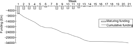
Figure 6.7 USD500 million funding requirement that has been arranged as three loans.
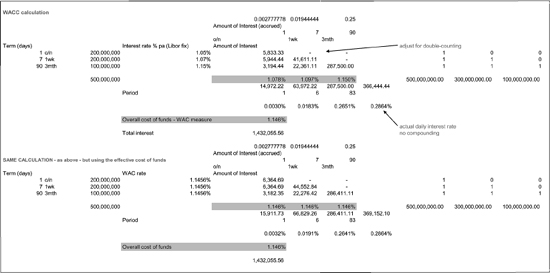
- overnight loan of USD200 million at 1.05%;
- 1-week loan of USD200 million at 1.07%;
- 3-month loan of USD100 million at 1.15%.
The spreadsheet shows the calculation of WACC on a more scientific basis than the ‘back of the envelope’ approach, as it takes into account the term structure effect of the loans (as we go further out along the term structure, we pay a higher rate of interest). However, the result is very close to the simple approach. The WACC for these three loans is shown to be 1.146%.
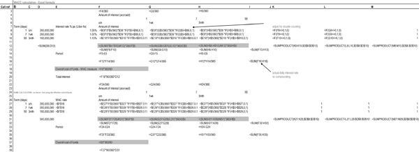
We repeat the spreadsheet at Figure 6.8 with the formulae used in each cell shown instead of the value.
Figure 6.8 Formulae used to calculate the USD500 million funding requirement that has been arranged as three loans.
SECURITIZATION
It is common for the ALM units in banks to take responsibility for a more proactive balance sheet management role; securitization is a good example of this. Securitization is a process undertaken by banks to both realize additional value from assets held on the balance sheet and to remove them from the balance sheet entirely, thus freeing up lending lines. Essentially, it involves selling assets on the balance sheet to third-party investors. In principle, the process is straightforward, as assets that are sold generate cashflows in the future, which provides return to investors who have purchased the securitized assets. To control risk exposure for investors, the uncertainty associated with certain asset cashflows is controlled or re-engineered – there are a range of ways in which this may be done.
For balance sheet management one of the principal benefits of securitisation is to save or reduce capital charges by the sale of assets. The other added benefit, of course, is that the process generates additional return for the issuing bank; therefore, securitization is not only a method by which capital charges may be saved, but an instrument in its own right that enables a bank to increase its return on capital.
The securitization process
For an introduction to asset-backed instruments see Fabozzi and Choudhry (2004). In this section we consider the implications of securitization from the point of view of asset and liability management. The subject is considered in greater detail in Choudhry (2007).
The basic principle of securitization is to sell assets to investors – usually through a medium known as a special purpose vehicle or some other intermediate structure – and to provide investors with a fixed or floating rate return on the assets they have purchased; the cashflows from the original assets are used to provide this return. It is rare, though not totally unknown, for investors to buy the assets directly; to avoid this, a class of securities is created to represent the assets and investors then purchase these securities. The most common types of assets securitized include mortgages, car loans and credit card loans. However, in theory, virtually any asset that generates a cashflow that can be predicted or modelled may be securitized. The vehicle used is constructed such that securities issued against the asset base have a risk return profile that is attractive to the investors being targeted.
To benefit from diversification, asset types are usually pooled and this pool then generates a range of interest payments, principal repayments and principal prepayments. The precise nature of cashflows is unclear not only because of the uncertainty of payment and prepayment patterns, but also because of the occurrence of loan defaults and delays in payment. However, pooling of a large number of loans means that cashflow fluctuation can be ironed out to a large extent, sufficient to issue notes against. The cashflows generated by the pool of assets are re-routed to investors by means of a dedicated structure, and a credit rating for the issue is usually requested from one or more private credit agencies. Most asset-backed securities carry investment-grade credit ratings – often triple A or double A – mainly because of various credit insurance facilities that are set up to guarantee the bonds. The securitization structure disassociates the quality of original cashflows from that of flows accruing to investors. In many cases, original borrowers are not aware that the process has occurred and notice no difference in the way their loan is handled. The credit rating on the securitization issue has no bearing on the rating of the selling bank and often will be different.
Benefits of securitization
Securitizing assets produces a double benefit for the issuing bank. Assets that are sold to investors generate a saving in the cost of required capital for the bank, as they are no longer on the balance sheet, so the bank’s capital requirement is reduced. Second, if the credit rating of the issued securities is higher than that of the originating bank, there is a potential gain in the funding costs of the bank. For example, if the securities issued are triple A rated, a double-A-rated bank will have lower funding costs for those securities. The bank benefits from paying a lower rate on the borrowed funds than if it had borrowed those funds directly in the market. This has led to strong growth in, for example, the specialized ‘credit card’ banks in the US, where banks such as Capital One, First USA and MBNA Bank have benefited from triple-A-rated funding levels and low capital charges. It is doubtful whether such banks could have grown as rapidly as they did without securitization. Although there is a cost associated with securitizing assets – which include direct issue transaction costs and the cost of running the payment structure – these are outweighed by the benefits obtained from the process.
The major benefit of securitization is reduced funding costs. Several factors influence such costs. These include
- Lower cost of funds due to the enhanced credit rating of the bonds issued. The extent of this gain is a function of current spreads in the market and the current rating of the originating bank. It will fluctuate in line with market conditions.
- Saving the capital charges that result from reducing the size of assets on the balance sheet. This decreases the minimum earnings required to ensure adequate return for shareholders, in effect improving return on capital at a stroke.
The costs of the process include
- Costs associated with setting up the issuing structure and, subsequently, the payment mechanism that channels cashflows to investors. These costs are a function of the structure and risk of the original assets; the higher the risk of the original assets, the higher the cost of ensuring cashflows for investors.
- The legal costs of origination, plus operating costs and servicing costs.
However, the reduction in funding cost obtained as a result of securitization should significantly outweigh the cost of the process itself. In order to determine whether securitization is feasible, as well as how it impacts return on capital, the originating bank will conduct a cost-and-benefit analysis prior to embarking on the process. This is frequently the responsibility of the ALM unit.
Example 6.1 Securitization transaction
We illustrate the impact of securitizing the balance sheet by an example from our hypothetical bank – ABC Bank plc.
The bank has a mortgage book of 100 million; the regulatory weight for this asset is 50%. The capital requirement is therefore 4 million – that is, 8%×0.5%×100 million. The capital is comprised of equity (estimated to cost 25%) and subordinated debt (which has a cost of 10.2%). The cost of straight debt is 10%. The ALM desk reviews a securitization of 10% of the asset book, or 10 million. The loan book has a fixed duration of 20 years, but its effective duration is estimated at 7 years, due to refinancings and early repayments. Net return from the loan book is 10.2%.
The ALM desk decides on a securitized structure that is made up of two classes of security: subordinated notes and senior notes. Subordinated notes will be granted a single A rating due to their higher risk, while senior notes are rated triple A. Given such ratings the required rate of return for subordinated notes is 10.61% and that of senior notes is 9.80%. Senior notes have a lower costthan current balance sheet debt, which has a cost of 10%. To
Table 6.5 ABC Bank plc mortgage loan book and securitization proposal
| Current funding | |
| Cost of equity | 25% |
| Cost of subordinated debt | 10.20% |
| Cost of debt | 10% |
| Mortgage book | |
| Net yield | 10.20% |
| Duration | 7 years |
| Balance outstanding | 100 million |
| Proposed structure | |
| Securitized amount | 10 million |
| Senior securities: | |
| Cost | 9.80% |
| Weighting | 90% |
| Maturity | 10 years |
| Subordinated notes: | |
| Cost | 10.61% |
| Weighting | 10% |
| Maturity | 10 years |
| Servicing costs | 0.20% |
obtain a single A rating, subordinated notes need to represent at least 10% of the securitized amount. The costs associated with the transaction are the initial cost of issue and the yearly servicing cost, estimated at 0.20% of the securitized amount. Summary information is given in Table 6.5.
A bank’s cost of funding is the average cost of all funds employed. The funding structure in our example is capital 4% – which is further split up as 2% equity at 25%, 2% subordinated debt at 10.20% and 96% debt at 10%. The weighted funding cost therefore is:

This average rate is consistent with the 25% before-tax return on equity given at the start. If the assets do not generate this return, the return received will change accordingly, since it is the end result of the bank’s profitability. As the assets only generate 10.20%, they are currently performing below shareholder expectations. The return actually obtained by shareholders is such that the average cost of funds is identical to the 10.20% return on assets. We may calculate this return to be:

Solving this relationship we obtain a return on equity (ROE) of 19.80%, which is lower than shareholder expectations. In theory, the bank would find it impossible to raise new equity in the market because its performance would not compensate shareholders for the risk they are incurring by holding the bank’s paper. Therefore, any asset that is originated by the bank would not only have to be securitized, but also be expected to raise shareholder return.
The ALM desk proceeds with securitization, issuing 9 million in senior securities and 1 million in subordinated notes. The bonds are placed by an investment bank with institutional investors. The outstanding balance of the loan book decreases from 100 million to 90 million. Weighted assets are therefore 45 million. Therefore, the capital requirement for the loan book is now 3.6 million, a reduction from the original capital requirement of 400,000, which can be used for expansion in another area (see Table 6.6).
Table 6.6 Impact of securitization on balance sheet
| Outstanding balances | Value (m) | Capital required (m) |
| Initial loan book | 100 | 4 |
| Securitized amount | 10 | 0.4 |
| Senior securities | 9 | Sold |
| Subordinated notes | 1 | Sold |
| New loan book | 90 | 3.6 |
| Total asset | 90 | |
| Total weighted assets | 45 | 3.6 |
The benefit of securitization is reduction in the cost of funding. Funding cost as a result of securitization is the weighted cost of senior notes and subordinated notes, together with the annual servicing cost. The cost of senior securities is 9.80%, while subordinated notes have a cost of 10.61% (for simplicity we ignore any differences in the duration and amortization profiles of the two bonds). This is calculated as:
![]()
This overall cost is lower than the target funding cost obtained directly from the balance sheet, which was 10.30%. This is the quantified benefit of the securitization process. Note that the funding cost obtained through securitization is lower than the yield on the loan book. Therefore, the original loan can be sold to the structure issuing the securities for a gain.
Example 6.2 Position management
Starting the day with a flat position, a money market interbank desk transacts the following deals:
1. 100 million borrowing from 16/9/09 to 7/10/09 (3 weeks) at 6.375%.
2. 60 million borrowing from 16/9/09 to 16/10/09 (1 month) at 6.25%.
3. 110 million loan from 16/9/09 to 18/10/09 (32 days) at 6.45%.
The desk reviews its cash position and the implications for refunding and interest rate risk, bearing in mind the following:
- There is an internal overnight rollover limit of 40 million (net).
- The bank’s economist feels more pessimistic about a rise in interest rates than most others in the market, and has recently given an internal seminar on the dangers of inflation in the UK as a result of recent increases in the level of average earnings.
- Today, some important figures are being released including inflation (RPI) data. If today’s RPI figures exceed market expectations, the dealer expects a tightening of monetary policy by at least 0.50% almost immediately.
- Brokers estimate daily market liquidity for the next few weeks to be one of low shortage, with little central bank intervention required, and hence low volatilities and low rates in the overnight rate.
- Brokers’ screens indicate the following term repo rates:
| O/N | 6.350%–6.300% |
| 1 week | 6.390%–6.340% |
| 2 week | 6.400%–6.350% |
| 1 month | 6.410%–6.375% |
| 2 month | 6.500%–6.450% |
| 3 month | 6.670%–6.620%. |
- The indication for a 1v2 FRA is:
| 1v2 FRA | 6.680%–6.630%. |
- The quote for an 11-day forward borrowing in 3 weeks’ time (the ‘21v32 rate’) is 6.50% bid.
The book’s exposure looks like this:

What courses of action are open to the desk, bearing in mind that the book needs to be squared off such that the position is flat each night?
Possible solutions
Investing early surplus
From a cash management point of view, the desk has a 50 million surplus from 16/9 up to 7/10. This needs to be invested. It may be able to negotiate a 6.31% loan with the market for overnight, or a 6.35% term deposit for 1 week or 6.38% for 1 month.
An overnight roll is the most flexible but offers the worst rate. If the desk expects the overnight rate to remain both low and stable (due to forecasts of low market shortages), it may not opt for this course of action.
However, it may make sense from an interest rate risk point of view. If the desk agrees with the bank’s economist, it should be able to benefit from rolling at higher rates soon – possibly in the next 3 weeks. Therefore, it may not want to lock in a term rate now, and the overnight roll would match this view. However, it exposes them to lower rates, if their view is wrong, which will limit the extent of the positive funding spread. The market itself appears neutral about rate changes in the next month, but appears to factor in a rise thereafter.
The forward ‘gap’
Looking forward, the book is currently on course to exceed the 40 million overnight position limit on 7/10, when the refunding requirement is 50 million. The situation gets worse on 16/10 (for 2 days) when the refunding requirement is 110 million. The desk needs to fix a term deal before those dates to carry it over until 18/10 when the funding position reverts to zero. A borrowing from 7/10 to 18/10 of 50 million will bring the rollover requirement back to within limits.
However, given that interest rates will rise, should the desk wait until the 7th to deal in the cash? Not if it has a firm view. It may end up paying as much as 6.91% or higher for the funding (after the 0.50% rate rise). So, it would be better to transact a forward-starting repo now to cover the period, thus locking in the benefits obtainable from today’s yield curve. The market rate for a 21×32-day repo is quoted at 6.50%. This reflects the market’s consensus that rates may rise in about a month’s time. However, the desk’s own expectation is of a larger rise – hence, its own logic suggests trading in the forward loan. This strategy will pay dividends if its view is right, as it limits the extent of funding loss.
An alternative means of protecting interest rate risk is to buy a 1v2-month FRA for 6.68%. This does not exactly match the gap, but should act as an effective hedge. If there is a rate rise, the book gains from the FRA profit. Note that the cash position still needs to be squared off. Should the desk deal before or after the inflation announcement? That is, of course, down to its own intuition, but most dealers like to sit tight ahead of releases of key economic data, if at all possible.
Generic ALM policy for different-sized banks
The management of interest rate risk is a fundamental ingredient of commercial banking. Bank shareholders take comfort from interest rate risk being measured and managed satisfactorily. A common approach to risk management involves the following:
- Preparation and adoption of a high-level interest rate risk policy at board level. This sets general guidelines on the type and extent of risk exposure that can be taken on by the bank.
- Setting limits on the risk exposure levels of the banking book. This can be by product type, desk, geographic area and so on, and will be along the maturity spectrum.
- Actively measuring the level of interest rate risk exposure at regular, specified intervals.
- Reporting to senior management on general aspects of risk management, risk exposure levels, limit breaches and so on.
- Monitoring risk management policies and procedures by an independent ‘middle office’ risk function.
The risk management approach adopted by banks will vary according to their specific markets and appetite for risk. Certain institutions have their activities set out or prescribed for them under regulatory rules. For instance, building societies in the UK are prohibited from trading in certain instruments by the regulator. In this section we present for illustrative purposes the ALM policies of three hypothetical banks: Bank S, Bank M and Bank L. These banks are, respectively, a small banking entity with assets of 500 million, a medium-sized bank with assets of 2.5 billion and a large bank with assets of 10 billion. In the following we demonstrate the differing approaches that can be taken according to the environment that a financial institution operates in.
ALM policy for Bank S (assets500 million)
The aim of the ALM policy for Bank S is to provide guidelines on risk appetite, revenue targets and rates of return, in addition to providing a risk management policy. Areas that may be covered include capital ratios, liquidity, asset mix, rate-setting policy for loans and deposits, as well as investment guidelines for the banking portfolio. The key objectives should include
- maintaining capital ratios at the planned minimum and ensuring the safety of the deposit base;
- generating a satisfactory revenue stream, both for income purposes and to further protect the deposit base.
The responsibility for overseeing the operations of the bank to ensure that these objectives are achieved is lodged with the ALCO. This body monitors the volume and mix of the bank’s assets and funding (liabilities), and ensures that this asset mix follows internal guidelines with regard to banking liquidity, capital adequacy, asset base growth targets, risk exposure and return on capital. The norm is for the committee to meet on a monthly basis; membership of the committee will include the finance director, the head of Treasury and the risk manager at the very least. For a bank the size of Bank S the ALCO membership will possibly be extended to the chief executive, the head of the loans business and the chief operating officer.
As a matter of course the committee will wish to discuss and review the following on a regular basis:
- Overall macroeconomic conditions.
- Financial results and key management ratios – such as share price analysis and rates of return on capital and equity.
- House view on the likely direction of short-term interest rates.
- Current lending strategy – and any suggestions for changes – and current funding strategy.
- Anticipated changes to the volume and mix of the loan book, and to that of the main sources of funding.
- Appropriateness or otherwise of alternative sources of funding.
- Suggestions for any alterations to the bank’s ALM policy.
- Maturity gap profile as well as anticipated and suggested changes to it.
The committee will also wish to consider interest rates currently offered on loans and deposits, and whether they are still appropriate.
Interest rate sensitivity is monitored and confirmed as lying within specified parameters; these parameters are regularly reviewed and adjusted if deemed necessary according to changes in the business cycle and economic conditions. Interest rate sensitivity is measured using the following ratio:
![]()
Typical risk levels would be expected to lie between 90% and 120% for the maturity period 0–90 days, and between 80% and 110% for the maturity period over 90 days but less than 365 days.
Put simply, the objective of Bank S is to remain within specified risk parameters at all times, and to maintain as consistent a level of earnings as possible (and one that is immune to changes in the business cycle).
ALM policy for Bank M (assets2.5 billion)
Bank M is our hypothetical ‘medium-sized’ banking institution. Its ALM policy would be overseen by the ALCO. Typically, the committee would consist of the following members of senior management:
- deputy chief executive
- finance director
- head of retail banking
- head of corporate banking
- head of Treasury
- head of risk management
- head of internal audit.
Others – such as product specialists – would be called to attend as and when required. The finance director often chairs the meeting.
The primary responsibilities of the ALCO are detailed below.
Objectives
The ALCO is tasked with reviewing the bank’s overall funding strategy. Decisions taken are recorded in the minutes and circulated to attendees and designated key staff. ALCO members are responsible for undertaking regular reviews of the following:
- minutes of the previous meeting;
- the ratio of interest-rate-sensitive assets to liabilities, gap reports, risk reports and the funding position;
- the bank’s view on the expected level of interest rates and how the book should be positioned in light of this;
- the ALCO view on anticipated funding costs in the short term and medium term – this is closely related to the previous item;
- stress-testing in the form of ‘what if?’ scenarios, to check the effect on the banking book of specified changes in market conditions;
- change in parameters that may be required if there is a change in market conditions or risk tolerance;
- current interest rates for loans and deposits, to ensure that they are in accordance with the overall lending and funding strategy;
- maturity distribution of the liquidity book (expected to be comprised of T-bills, CDs and very short-dated government bonds);
- current liquidity position and expected position in the short term and medium term.
As the ALCO meets on a regular monthly basis, it is usual for only a few of these aspects to be discussed at every meeting; the agenda is set by the chair of the meeting in consultation with committee members. The policies adopted by the ALCO should be dynamic and flexible, and capable of adaptation to changes in operating conditions. Any changes to policy can only be made by the committee itself and any exceptions to agreed policy can only be made with the approval of the CEO or the ALCO itself.
Interest rate risk policy
The objective will be to keep earnings volatility resulting from an upward or downward move in interest rates to a minimum. To this end, at each ALCO meeting members will review risk and position reports and discuss them in light of the risk policy. Generally, the 6-month and 12-month cumulative ratio will lie in the range 90% to 110%. A significant move outside this range will most likely be subject to corrective action. The committee will also consider the results of various scenario analyses on the book, and if these tests indicate a potential earnings impact of greater than, say, 10%, instructions may be given to alter the shape and maturity profile of the book.
Liquidity policy
A primary responsibility of the ALCO is to ensure that an adequate level of liquidity is maintained at all times. Gup and Brooks (1993, p. 238) define liquidity as the ability to meet anticipated and unanticipated operating cash needs, loan demand, and deposit withdrawals, without incurring a sustained negative impact on profitability.’
Generally, a Bank-M-type operation would expect to have a target level for loans to deposits of around 75% to 85%, and a loans-to-core-deposits ratio of 85% to 95%. The loan/deposit ratio is reported to the ALCO and reviewed on a monthly basis, and any reported figure significantly outside these ranges (say, by 5% or more) will be reviewed and asked to be adjusted to bring it back into line with ALCO policy.
ALM policy for Bank L (assets10 billion)
The policy for ALM at a larger entity will build on that described for a medium-sized financial institution. If Bank L is a group company, the policy will cover the consolidated balance sheet as well as individual subsidiary balance sheets; the committee will provide direction on the management of assets and liabilities as well as on the off-balance-sheet instruments used to manage interest rate and credit risk. A well-functioning management process will be proactive and concentrate on direction in response to anticipated changes in operating conditions, rather than reactive responses to changes that have already taken place. Primary objectives will be to maximize shareholder value, with target returns on capital of 15% to 22%.
The responsibility for implementing and overseeing ALM policy will reside with the ALCO. The committee will establish operating guidelines for ALM and review them periodically. It will meet on a more frequent basis than is the case for Bank M – usually fortnightly. In addition to this, it will set policies governing liquidity and funding objectives, investment activities and interest rate risk. It will also oversee the activities of the investment-banking division. The head of the ALM desk will prepare the interest rate risk sensitivity report and present it to the ALCO.
Interest rate risk management
The ALCO will establish an interest rate risk policy that sets the direction for acceptable levels of interest rate risk. This risk policy is designed to help management evaluate the impact of interest rate risk on the bank’s earnings. The extent of risk exposure is a function of the maturity profile of the balance sheet, as well as the frequency of repricing, the level of loan prepayments and funding costs. Managing interest rate risk is, in effect, the adjustment of risk exposure upwards or downwards in response to the ALCO’s views on the future direction of interest rates. As part of the risk management process the committee will monitor current risk exposure and the duration gap, using rate sensitivity analysis and simulation modelling to assess whether the current level of risk is satisfactory.
Measuring interest rate risk
Notwithstanding the widespread adoption of value-at-risk as the key market risk measurement tool, funding books such as repo books continue to use the gap report as a key measure of interest rate risk exposure. This enables the ALCO to view risk sensitivity along the maturity structure. Cumulative gap positions and the ratio of asset revaluation to liability revaluation are calculated and compared with earnings levels on the current asset/liability position. Generally, the 90-day, 6-month and 1-year gap positions are the most significant points along the term structure at which interest rate risk exposure is calculated. The ratio of gap to earnings assets is set at the 15% to 20% level.
As it is a traditional duration-based approach, gap reporting is a static measure for risk sensitivity at one specific point in time. It is for this reason that banks combine a value-at-risk measure as well, or use it exclusively. It is outside the scope of this book to consider VaR – we cite a useful introductory reference at the end of this chapter (Butler, 1998).
Simulation modelling
Simulation modelling is a procedure that measures potential impact on the banking book – and hence earnings levels – of a user-specified change in interest rates and/or a change in the shape of the book itself. This process enables senior management to gauge the risk associated with particular strategies. Put simply the process involves
- Constructing a ‘base’ balance sheet and income statement as the starting point (this is derived from the current shape of the banking book and any changes expected from current growth trends that have been projected forward).
- Assessing the impact on the balance sheet of changes under selected scenarios: say, no change in rates; a 100bp and 250bp upward parallel shift in the yield curve; a 100bp and 250bp downward parallel shift; a 25bp steepening and flattening of the yield curve between the 5-month and the 3-year maturity points; a combination of parallel shift with pivotal shift at a selected point; an increase or decrease in 3-month T-bill yield volatility levels; and a 20bp change in swap spreads.
- Comparing the difference in earnings resulting from any of the scenarios to the anticipated earnings stream under the current environment.
Generally, the committee sets guidelines about the significance of simulation results; for example, there may be a rule that for a 100bp change in interest rates the impact on NII should be no more than 10%. If results indicate such an impact, the ALCO will determine whether the current risk strategy is satisfactory or whether adjustments are necessary.
NPV AND VALUE-AT-RISK
The NPV of a banking book is an appropriate target of interest rate policy because it captures all future cashflows and is equal to the discounted value of future margins when the discount rate is the cost of all debt. The sensitivity of NPV is derived from the duration of assets and liabilities. Therefore, we may write the change in NPV as:
where is the duration of assets and is the market value of assets. Equation (6.6) is applicable when only one interest rate is used for reference. Sensitivity with respect to interest rate is known. It is then possible to derive value-at-risk (VaR) from these simple relationships. With one interest rate we are interested in the maximum variation of NPV that results from a change in the reference interest rate. NPV volatility can be derived from its sensitivity and from interest rate volatility. If we set as the sensitivity of NPV to interest rate, NPV volatility is given by:
(6.7) ![]()
Once volatility is known, maximum change at a given confidence level is obtained as a multiple of volatility. The multiple is based on assumptions with respect to the shape of the distribution of interest rates. Under a curve with normal distribution, a multiple of 1.96 provides maximum expected change at a 2.5% two-tailed confidence level, so that we are able to say that the VaR of the book is as given by:
(6.8) ![]()
Where there is more than one interest rate, variation in NPV can be approximated as a linear combination of variations due to the change in each interest rate. This is written as:
(6.9) ![]()
where, and are the different interest rates. Since all interest rate changes are uncertain, NPV volatility is the volatility of a sum of random variables. Deriving the volatility of this sum requires assumptions on correlations between interest rates.
This problem is identical to the general problem of measuring the market risk of a portfolio when mindful that its change in market value arises as a result of changes generated by random variations of market parameters. The main concern is to calculate the volatility of the mark-to-market value of the portfolio, expressed as the sum of random changes of mark-to-market values of the various individual transactions. These random changes can be interdependent, in the same way that underlying market parameters are. Volatility in the value of the portfolio depends upon the sensitivities of individual transactions, upon the volatilities of individual market parameters and upon their interdependency, if any exists. The methodology that calculates this volatility is known as delta-VaR. This is based on the delta sensitivity of the portfolio to changes in market interest rates.
BIBLIOGRAPHY
Anon. (1998) Asset and Liability Management, RISK Publications.
Bitner, J. (1992) Successful Bank Asset–Liability Management, John Wiley & Sons.
Butler, C. (1998) Mastering Value-at-Risk, FT/Prentice Hall.
Choudhry, M. (2007) Bank Asset and Liability Management, Singapore: John Wiley & Sons.
Cornyn, A. and Mays, E. (Eds.) (1997) Interest Rate Risk Models: Theory and Practice, Glenlake Publishing/Fitzroy Dearborn Publishers, Chapters 6 and 15
Fabozzi, F. and Choudhry, M. (2004) Handbook of European Structured Financial Products, John Wiley & Sons.
Fabozzi, F. and Konishi, A. (1996) The Handbook of Asset/Liability Management, Revised Edition, Irwin McGraw-Hill, Chapters 3, 6–8, 12.
Greenbaum, S. and Thakor, A. (1995) Contemporary Financial Intermediation, Dryden Press.
Gup, B. and Brooks, R. (1993) Interest Rate Risk Management, Irwin Professional Publishing.
Howe, D. (1992) A Guide to Managing Interest-Rate Risk, New York Institute of Finance.
Johnson, H. (1994) Bank Asset/Liability Management, Probus Publishing.
Kamakura Corporation (1998) Asset & Liability Management: A Synthesis of New Methodologies, Risk Publications.
Koch, T. (1988) Bank Management, Dryden Press.
Marshall, J. and Bansal, V.K. (1992) Financial Engineering, New York Institute of Finance, Chapter 20
Schaffer, S. (1991) ‘Interest Rate Risk,’ Business Review, Federal Reserve Bank of Philadelphia, May/June, 17–27
Sinkey, J. (1992) Commercial Bank Financial Management, Fourth Edition, Macmillan.
Stevenson, B. and Fadil, M. (1995) ‘M#odern Portfolio Theory: Can it work for commercial loans?’ Commercial Lending Review, 10(2), Spring, 4–12.
Toevs, A. and Haney, W. (1984) Measuring and Managing Interest Rate Risk, Morgan Stanley.
Toevs, A. and Haney, W. (1986) ‘Measuring and managing interest rate risk: A guide to asset/liability models used in banks and thrifts,’ in R. Platt (Ed.), Controlling Interest Rate Risk: New Techniques and Applications for Money Management, John Wiley & Sons.
Wilson, J.S.G. (Ed.) (1988) Managing Banks’ Assets and Liabilities, Euromoney Publications.
1 In this chapter the term liquidity is used to refer to funding liquidity.
2 The Economist, 30 October 1999.
3 For instance, in the US banking sector terms on deposit accounts were fixed by regulation, and there were restrictions on the geographic base of customers and the interest rates that could be offered. Interest rate volatility was also low. In this environment ALM consisted primarily of asset management, in which the bank would use depositors’ funds to arrange the asset portfolio that was most appropriate for the liability portfolio. This involved little more than setting aside some of the assets in non-interest reserves at the central bank and investing the balance in short-term securities, while any surplus would be lent out at very-short-term maturities.
4 The marketability definition of liquidity is also important in ALM. Less liquid financial instruments must offer a yield premium that can be compared with liquid instruments.
5 Or is proved to be correct at least three times out of five!
6 This describes a barbell structure, but this is really a bond market term.
7 This assumes a conventional upward-sloping yield curve.