
Chapter 4
INTRODUCTION TO TRADING AND HEDGING
In this chapter we introduce the basics of trading and hedging as employed by a bank asset–liability management (ALM) desk. The instruments and techniques used form the fundamental building blocks of ALM, so the reader can imagine that a full and comprehensive treatment of this subject would require a book in its own right.1 Our purpose here is to acquaint the newcomer to the market with the essentials, with further recommended reading suggested in the Bibliography.
The ALM and money market desk has a vital function in a bank, funding all the business lines in the bank. In some banks and securities houses it will be placed within the Treasury or money market areas, whereas other firms will organize it as an entirely separate function. Wherever it is organized, the need for clear and constant communication between the ALM desk and the other operating areas of the bank is paramount. We present an overview of ALM, liquidity and interest rate strategy in the next chapter; here we look at specific uses of money market products like deposits and repo in the context of yield enhancement and market-making.
TRADING APPROACH
The yield curve and interest rate expectations
When the yield curve is positively sloped, the conventional approach is to fund the book at the short end of the curve and lend at the long end. In essence, therefore, if the yield curve resembled that shown in Figure 4.1 a bank would borrow, say, 1-week funds while simultaneously lending out at, say, 3-month maturity. This is known as funding short. A bank can effect the economic equivalent of borrowing at the short end of the yield curve and lending at the longer end through repo transactions – in our example, a 1-week repo and a 3-month reverse repo. The bank then continuously rolls over its funding at 1-week intervals for the 3-month period. This is also known as creating a tail; here the ‘tail’ is the gap between 1 week and 3 months – the interest rate ‘gap’ that the bank is exposed to. During the course of the trade – as the reverse repo has locked in a loan for 6 months – the bank is exposed to interest rate risk should the slope or shape of the yield curve change. In this case the bank may see its profit margin shrink or turn into a funding loss if short-dated interest rates rise.
Figure 4.1 Positive yield curve funding.
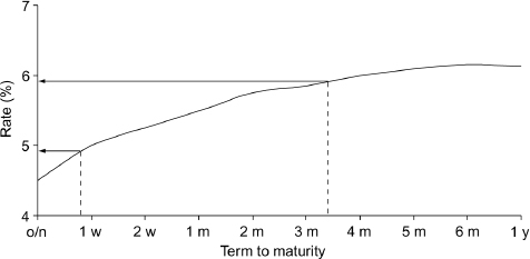
As we noted in Chapter 3, a number of hypotheses have been advanced to explain the shape of the yield curve at any particular time. A steep positive-shaped curve may indicate that the market expects interest rates to rise over the longer term, although this is also sometimes given as the reason for an inverted curve with regard to shorter term rates. Generally speaking, trading volumes are higher in a positive-sloping yield curve environment, compared with a flat or negative-shaped curve.
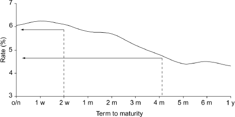
In the case of an inverted yield curve, a bank will (all else being equal) lend at the short end of the curve and borrow at the longer end. This is known as funding long and is shown in Figure 4.2.
The example in Figure 4.2 shows a short cash position of 2-week maturity against a long cash position of 4-month maturity. The interest rate gap of 10 weeks is the book’s interest rate exposure. The inverted shape of the yield curve may indicate market expectations of a rise in short-term interest rates. Further along the yield curve, the market may expect a benign inflationary environment, which is why the premium on longer term returns is lower than normal.
Figure 4.2 Negative yield curve funding.
Credit intermediation by the repo desk
The government bond repo market will trade at a lower rate than other money market instruments, reflecting its status as a secured instrument with the best credit. This allows spreads between markets of different credits to be exploited. The following are examples of credit intermediation trades:
- a repo dealer lends general collateral currently trading at a spread below Libor and uses the cash to buy CDs trading at a smaller spread below Libor;
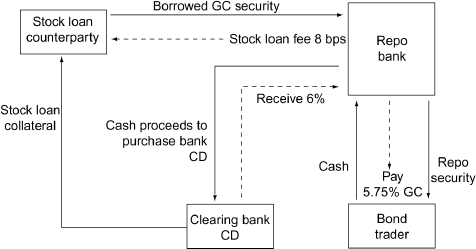
- a repo dealer borrows specific collateral in the stock-lending market – paying a fee – and sells the stock in the repo market at the GC rate; the cash is then lent in the interbank market at a higher rate – for instance, through the purchase of a clearing bank certificate of deposit. The CD is used as collateral in the stock loan transaction. A bank must have dealing relationships with both the stock loan and repo markets to effect this trade. An example of the trade that could be put on using this type of intermediation is shown in Figure 4.3 for the UK gilt market. The details are given below and show that the bank would stand to gain 17 basis points over the course of the 3-month trade;
- a repo dealer trades repo in the GC market, and using the cash from this repo invests in emerging market collateral at a spread, say, 400 basis points higher.
Figure 4.3 Intermediation between stock loan and repo markets; an example using UK gilts.
These are but three examples of the way that repo can be used to exploit the interest rate differentials that exist between markets of varying credit qualities and between secured and unsecured markets.
Figure 4.3 shows potential gains that can be made by a repo-dealing bank (market-maker) that has access to both the stock loan and general collateral repo market. It illustrates the rates available in the gilt market on 31 October 2000 for 3-month maturities, which were
| 3-month GC repo | 5.83–5.75% |
| 3-month clearing bank CD | 6–6.00% |
The stock loan fee for this term was quoted at 5?10 basis points, with the actual fee paid being 8 basis points. Therefore, the repo trader borrows GC stock for 3 months and offers this in repo at 5.75%;2 the cash proceeds are then used to purchase a clearing bank CD at 6.00%. This CD is used as collateral in the stock loan. The profit is market risk-free as the terms are locked, although there is an element of credit risk in holding the CD. On these terms, the profit in 100 million stock for the 3-month period is approximately 170,000.
The main consideration for the dealing bank is the capital requirements of the trade. Gilt repo is zero-weighted for capital purposes; indeed, clearing bank CDs are accepted by the Bank of England for liquidity purposes, so the capital cost is not onerous. The bank will need to ensure that it has sufficient credit lines for the repo and CD counterparties.
SPECIALS TRADING
The existence of an open repo market allows the demand for borrowing and lending stocks to be cleared by the price mechanism – in this case the repo rate. This facility also measures supply and demand for stocks more efficiently than traditional stock lending. It is to be expected that – when specific stocks are in demand – the premium on obtaining them rises for a number of reasons. This is reflected in the repo rate associated with the specific stock in demand, which falls below the same maturity GC repo rate. The repo rate falls because the entity repoing out stock – that is, borrowing cash – is in possession of the desired asset: the specific bond. So, the interest rate payable by this counterparty falls as compensation for lending out the desired bond.
The factors contributing to individual securities becoming special include
- government bond auctions; the bond to be issued is shorted by market-makers in anticipation of a new supply of stock and due to client demand;
- outright short-selling, whether deliberate position-taking on the trader’s view, or market-makers selling stock on client demand;
- hedging, including bond underwriters who will short the benchmark government bond that the corporate bond is priced against;
- derivatives trading such as basis (‘cash-and-carry’) trading creating demand for a specific stock.
Natural holders of government bonds can benefit from issues going special, which is when the demand for specific stocks is such that the rate for borrowing them is reduced. The lower repo rate reflects the premium for borrowing the stock. Note that the party borrowing the special stock is lending cash; it is the rate payable on the cash that they have lent which is depressed.
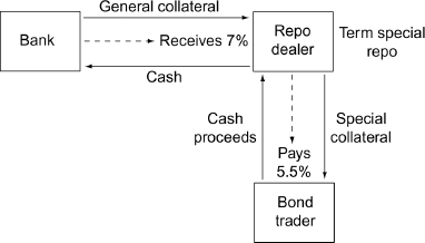
The holder of a stock that has gone special can obtain cheap funding for the issue itself by lending it out. Alternatively, the holder can lend the stock and obtain cash in exchange in a repo, for which the rate payable is lower than the interbank rate. These funds can then be lent out as either secured funding (in a repo), or as unsecured funding, enabling the specials holder to lock in a funding profit. For example, consider a situation where a repo dealer holds an issue that is trading at 5.5% in 1-week repo. The equivalent GC rate is 7%, making the specific issue very special. By lending the stock out the dealer can lock in the profit by lending 1-week cash at 7% or at a higher rate in the interbank market. This is illustrated in Figure 4.4.
Figure 4.4 Funding gain from repo of a special stock.
There is a positive correlation between changes in a stock trading expensive to the yield curve and changes in the degree to which it trades special. Theory would predict this, since traders will maintain short positions for bonds with high funding (repo) costs only if the anticipated fall in the price of the bond is large enough to cover this funding premium. When stock is perceived as being expensive – for example, after an auction announcement – this creates a demand for short positions and hence greater demand for the paper in a repo. At other times the stock may go tight in the repo market, following which it will tend to be bid higher in the cash market as traders close out existing shorts (which had become expensive to finance). At the same time traders and investors may attempt to buy the stock outright since it will now be cheap to finance in a repo. The link between dearness in the cash market and special status in the repo market flows both ways.
MATCHED BOOK TRADING
The growth and development of repo markets has led to repo matched-book-trading desks. Essentially, this is market-making in repo; dealers make two-way trading prices in various securities, irrespective of their underlying positions. The term ‘matched book’ is in fact a misnomer; most matched books are deliberately mismatched as part of a view on the short-term yield curve. Another commonly encountered definition of the term is of a bank that trades repo solely to cover its long and short bond positions and does not enter into trades for other reasons.3 However, it is not matching cash lent and borrowed, nor trading to profit from the bid–offer spread, nor any of the sundry other definitions that have been given in previous texts.
Traders running a matched book put on positions to take advantage of (i) short-term interest rate movements and (ii) anticipated supply and demand in the underlying stock. Many of the trading ideas and strategies described in this book are examples of matched book trading. It can involve the following types of trade:
- taking a view on interest rates – for example, the dealer bids for 1-month GC and offers 3-month GC, expecting the yield curve to invert;
- taking a view on specials – for example, the trader borrows stock in the stock-lending market for use in repo once it goes special (as the trader expects);
- credit intermediation – for example, a dealer reverses in Brady bonds from a Latin American bank, at a rate of Libor200 and offers this stock to a US money market investor at a rate of Libor20.
Principals and principal intermediaries with large volumes of repos and reverse repos, such as the market-makers mentioned above, are said to be running matched books. An undertaking to provide two-way prices is made to provide customers with a continuous financing service for long and short positions and also as part of proprietary trading. Traders will mismatch positions in order to take advantage of a combination of two factors: short-term interest rate movements and anticipated supply/demand in the underlying bond.
INTEREST-RATE-HEDGING TOOLS
For bank dealers who are not looking to trade around term mismatch or other spreads, but who will run a tenor mismatch between assets and liabilities (which is, after all, what banking is: the practice of maturity transformation), there are a number of instruments we can use to hedge the resulting interest rate risk exposure. We briefly consider them here. They are covered in greater depth in Choudhry (2007).
Interest rate futures
A forward term interest rate gap exposure can be hedged using interest rate futures. These are standardized exchange-traded derivative contracts, and represent a forward-starting 90-day time deposit. In the sterling market the instrument will be typically the 90-day short sterling future traded on the LIFFE futures exchange. A strip of futures can be used to hedge the term gap. The trader buys futures contracts to the value of the exposure and for the term of the gap. Any change in cash rates should be hedged by offsetting moves in futures prices.
Description
A futures contract is a transaction that fixes the price today for a commodity that will be delivered at some point in the future. Financial futures fix the price for interest rates, bonds, equities and so on, but trade in the same manner as commodity futures. Contracts for futures are standardized and traded on recognized exchanges. In London the main futures exchange is LIFFE, although other futures are also traded on, for example, the International Petroleum Exchange and the London Metal Exchange. Money markets trade short-term interest rate futures that fix the rate of interest on a notional fixed term deposit of money (usually for 90 days or 3 months) for a specified period in the future. The sum is notional because no actual sum of money is deposited when buying or selling futures – the instrument being off balance sheet. Buying such a contract is equivalent to making a notional deposit, while selling a contract is equivalent to borrowing a notional sum.
The 3-month interest rate future is the most widely used instrument for hedging interest rate risk.
The LIFFE exchange in London trades short-term interest rate futures for major currencies including sterling, euros, yen and the Swiss franc. Table 4.1 summarizes the terms for the short sterling contract as traded on LIFFE.
Table 4.1 Description of LIFFE short sterling future contract
| Name | 90-day sterling Libor interest rate future |
| Contract size | 500,000 |
| Delivery months | March, June, September, December |
| Delivery date | First business day after the last trading day |
| Last trading day | Third Wednesday of delivery month |
| Price | 100 minus interest rate |
| Tick size | 0.01 |
| Tick value | 12.50 |
| Trading hours | LIFFE CONNECTTM 07:3018:00 hours |
| Source: LIFFE. | |
Futures contracts originally related to physical commodities, which is why we speak of delivery when referring to the expiry of financial futures contracts. Exchange-traded futures such as those on LIFFE are set to expire every quarter during the year. The short sterling contract is a deposit of cash, so as its price refers to the rate of interest on this deposit the price of the contract is set as where is the price of the contract and is the rate of interest at the time of expiry implied by the futures contract. This means that if the price of the contract rises the rate of interest implied goes down and vice versa. For example, the price of the June 2011 short sterling future (written as Jun11 or M11, from the futures identity letters of H, M, U and Z for contracts expiring in March, June, September and December, respectively) at the start of trading on 22 September 2010 was 99.05, which implied a 3-month Libor rate of 0.95% on expiry of the contract in June 2011. If a trader bought 20 contracts at this price and then sold them just before the close of trading that day, when the price had risen to 99.08, an implied rate of 0.92%, she would have made 3 ticks profit or 750. That is, a 3-tick upward price movement in a long position of 20 contracts is equal to 750. This is calculated as follows:
![]()
The tick value for the short sterling contract is straightforward to calculate. Since we know that the contract size is 500,000, there is a minimum price movement (tick movement) of 0.01% and the contract has a 3-month ‘maturity’:
![]()
The profit made by the trader in our example is logical because if we buy short sterling futures we are depositing (notional) funds and if the price of the futures rises, it means the interest rate has fallen. We profit because we have ‘deposited’ funds at a higher rate beforehand. If we expected sterling interest rates to rise, we would sell short sterling futures, which is equivalent to borrowing funds and locking in the loan rate at a lower level.
Note how the concept of buying and selling interest rate futures differs from FRAs: if we buy a FRA we are borrowing notional funds, whereas if we buy a futures contract we are depositing notional funds. If a position in an interest rate futures contract is held to expiry, cash settlement will take place on the delivery day for that contract.
Short-term interest rate contracts in other currencies are similar to the short sterling contract and trade on exchanges such as Deutsche Terminboörse in Frankfurt and MATIF in Paris.
In practice, futures contracts do not provide a precise tool for locking into cash market rates today for a transaction that takes place in the future, although this is what they are theoretically designed to do. Futures do allow a bank to lock in a rate for a transaction to take place in the future; this rate is the forward rate. The basis is the difference between today’s cash market rate and the forward rate on a particular date in the future. As a futures contract approaches expiry, its price and the rate in the cash market will converge (the process is given the name convergence). This is given by the exchange delivery settlement price, and the two prices (rates) will be exactly in line at the precise moment of expiry.
Example 4.1 The Eurodollar futures contract
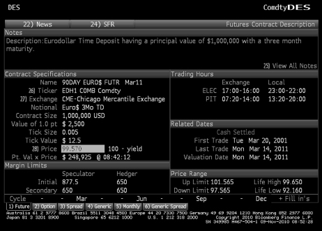
The Eurodollar futures contract is traded on the Chicago Mercantile Exchange. The underlying asset is a deposit of US dollars in a bank outside the US, and the contract is at the rate of dollar 90-day Libor. The Eurodollar future is cash-settled on the second business day before the third Wednesday of the delivery month (London business day). The final settlement price is used to set the price of the contract, given by
![]()
where is the quoted Eurodollar rate at the time. This rate is the actual 90-day Eurodollar deposit rate.
The longest dated Eurodollar contract has an expiry date of 10 years. The market assumes that futures prices and forward prices are equal; this is indeed the case under conditions where the risk-free interest rate is constant and the same for all maturities. In practice, it also holds for short-dated futures contracts, but does not for longer dated futures contracts. Therefore, using futures contracts with a maturity greater than 5 years to calculate zero-coupon rates or implied forward rates will produce errors in results, which need to be taken into account if the derived rates are used to price other instruments such as swaps.
Figure 4.5 shows the Bloomberg description page for the Eurodollar contract.
Hedging using interest rate futures
Banks use interest rate futures to hedge interest rate risk exposure in cash and OBS instruments. Bond-trading desks often use futures to hedge positions in bonds of up to 2 or 3 years’ maturity, as contracts are traded up to 3 years’ maturity. The liquidity of such ‘far month’ contracts is considerably lower than for ‘near month’ contracts and the ‘front month’ contract (the current contract, for the next maturity month). When hedging a bond with a maturity of say 2 years’ maturity, the trader will put on a strip of futures contracts that matches as near as possible the expiry date of the bond.
The purpose of a hedge is to protect the value of a current or anticipated cash market or OBS position from adverse changes in interest rates. The hedger will try to offset the effect of the change in interest rate on the value of his cash position with the change in value of his hedging instrument. If the hedge is an exact one the loss on the main position should be compensated by a profit on the hedge position. If the trader is expecting a fall in interest rates and wishes to protect against such a fall he will buy futures (known as a long hedge) and will sell futures (a short hedge) if wishing to protect against a rise in rates.
Bond traders also use 3-month interest rate contracts to hedge positions in short-dated bonds; for instance, a market-maker running a short-dated bond book would find it more appropriate to hedge his book using short-dated futures rather than the longer dated bond futures contract. When this happens it is important to accurately calculate the correct number of contracts to use for the hedge. To construct a bond hedge it will be necessary to use a strip of contracts, thus ensuring that the maturity date of the bond is covered by the longest dated futures contract. The hedge is calculated by finding the sensitivity of each cashflow to changes in each of the relevant forward rates. Each cashflow is considered individually and hedge values are then aggregated and rounded to the nearest whole number of contracts.
Examples 4.2 and 4.3 illustrate hedging with short-term interest-rate contracts.
Examples 4.2 Hedging a forward 3-month lending requirement
On 1 June a corporate treasurer is expecting a cash inflow of 10 million in 3 months’ time (1 September), which he will then invest for 3 months. The treasurer expects interest rates will fall over the next few weeks and wishes to protect himself against such a fall. This can be done using short sterling futures. The market rates on 1 June are as follows:
![]()
The treasurer buys 20 September short sterling futures at 93.220, this number being exactly equivalent to a sum of 10 million. This allows him to lock in a forward lending rate of 6.78%, on the assumption there is no bid–offer quote spread:
On 1 September the market rates are as follows:
![]()
The treasurer unwinds the hedge at this price.
![]()
Effective lending rate = 3-month Libor Futures profit
![]()
The treasurer was quite close to achieving his target lending rate of 6.78% and the hedge has helped to protect against the drop in Libor rates from 6 1/2% to 6 1/4%, as a result of the profit from the futures transaction.
In the real world the cash market bid–offer spread will impact the amount of profit/loss from the hedge transaction. Futures generally trade and settle near the offered side of the market rate (Libor) whereas lending, certainly by corporates, will be nearer the Libid rate.
Example 4.3 Hedging a forward 6-month borrowing requirement
A Treasury dealer has a 6-month borrowing requirement for EUR30 million in 3 months’ time, on 16 September. He expects interest rates to rise by at least 1/2% before that date and would like to lock in a future borrowing rate. The scenario is:
| Date | 16 June |
| 3-month LIBOR | 6.0625% |
| 6-month LIBOR | 6.25 |
| Sep futures contract | 93.66 |
| Dec futures contract | 93.39 |
In order to hedge a 6-month DEM30 million exposure the dealer needs to use a total of 60 futures contracts, as each has a nominal value of EUR1 million, and corresponds to a 3-month notional deposit period. The dealer decides to sell 30 September futures contracts and 30 December futures contracts. This is referred to as a strip hedge. The expected forward borrowing rate that can be achieved by this strategy, where the expected borrowing rate is, is calculated as follows:
Therefore, we have:
The rate is sometimes referred to as the ‘strip rate’.
The hedge is unwound upon expiry of the September futures contract. Assume the following rates now prevail:
| 3-month LIBOR | 6.4375% |
| 6-month LIBOR | 6.8125 |
| Sep futures contract | 93.56 |
| Dec futures contract | 92.93 |
The futures P&L is:
| September contract | 10 ticks |
| December contract | 46 ticks |
This represents a 56-tick or 0.56% profit in 3-month interest rate terms, or 0.28% in 6-month interest rate terms. The effective borrowing rate is the 6-month LIBOR rate minus the futures profit, or:
![]()
In this case the hedge has proved effective because the dealer has realized a borrowing rate of 6.5325%, which is close to the target strip rate of 6.53%.
The dealer is still exposed to the basis risk when the December contracts are bought back from the market at the expiry date of the September contract. If, for example, the future was bought back at 92.73, the effective borrowing rate would only be 6.4325%, and the dealer would benefit. Of course, the other possibility is that the futures contract could be trading 20 ticks more expensive, which would give a borrowing rate of 6.6325%, which is 10 basis points above the target rate. If this happened, the dealer may elect to borrow in the cash market for 3 months, maintain the December
futures position until the December contract expiry date, and roll over the borrowing at that time. The profit (or loss) on the December futures position will compensate for any change in 3-month rates at that time.
Forward rate agreements
Forward rate agreements (FRAs) are similar in concept to interest rate futures and like them are off-balance-sheet instruments. Under a FRA a buyer agrees notionally to borrow and a seller to lend a specified notional amount at a fixed rate for a specified period – the contract to commence on an agreed date in the future. On this date (the ‘fixing date’) the actual rate is taken and, according to its position versus the original trade rate, the borrower or lender will receive an interest payment on the notional sum equal to the difference between the trade rate and the actual rate. The sum paid over is present-valued as it is transferred at the start of the notional loan period, whereas in a cash market trade interest would be handed over at the end of the loan period. As FRAs are off-balance-sheet contracts no actual borrowing or lending of cash takes place, hence the use of the term ‘notional’. In hedging an interest rate gap in the cash period, the trader will buy a FRA contract that equates to the term gap for a nominal amount equal to his exposure in the cash market. Should rates move against him in the cash market, the gain on the FRA should (in theory) compensate for the loss in the cash trade.
Definition of a FRA
A FRA is an agreement to borrow or lend a notional cash sum for a period of time lasting up to 12 months, starting at any point over the next 12 months, at an agreed rate of interest (the FRA rate). The ‘buyer’ of a FRA is borrowing a notional sum of money while the ‘seller’ is lending this cash sum. Note how this differs from all other money market instruments. In the cash market, the party buying a CD or bill, or bidding for stock in the repo market, is the lender of funds. In the FRA market, to ‘buy’ is to ‘borrow’. Of course, we use the term ‘notional’ because with a FRA no borrowing or lending of cash actually takes place. The notional sum is simply the amount on which interest payment is calculated.
So, when a FRA is traded, the buyer is borrowing (and the seller is lending) a specified notional sum at a fixed rate of interest for a specified period – the ‘loan’ to commence at an agreed date in the future. The buyer is the notional borrower, and so she will be protected if there is a rise in interest rates between the date that the FRA is traded and the date that the FRA comes into effect. If there is a fall in interest rates, the buyer must pay the difference between the rate at which the FRA was traded and the actual rate, as a percentage of the notional sum. The buyer may be using the FRA to hedge an actual exposure – that is, an actual borrowing of money – or simply speculating on a rise in interest rates. The counterparty to the transaction, the seller of the FRA, is the notional lender of funds, and has fixed the rate for lending funds. If there is a fall in interest rates the seller will gain, and if there is a rise in rates the seller will pay. Again, the seller may have an actual loan of cash to hedge or be a speculator.
In FRA trading only the payment that arises as a result of the difference in interest rates changes hands. There is no exchange of cash at the time of the trade. The cash payment that does arise is the difference in interest rates between that at which the FRA was traded and the actual rate prevailing when the FRA matures, as a percentage of the notional amount. FRAs are traded by both banks and corporates and between banks. The FRA market is very liquid in all major currencies and rates are readily quoted on screens by both banks and brokers. Dealing is over the telephone or over a dealing system such as Reuters.
The terminology quoting FRAs refers to the borrowing time period and the time at which the FRA comes into effect (or matures). Hence, if a buyer of a FRA wished to hedge against a rise in rates to cover a 3-month loan starting in 3 months’ time, she would transact a ‘3-against-6-month’ FRA, more usually denoted as a 3×6 or 3v6 FRA. This is referred to in the market as a ‘threes–sixes’ FRA, and means a 3-month loan beginning in 3 months’ time. So, correspondingly, a ‘ones–fours’ FRA (1v4) is a 3-month loan in 1 month’s time, and a ‘threes–nines’ FRA (3v9) is a 6-month loan in 3 months’ time.
Remember that when we buy a FRA we are ‘borrowing’ funds. This differs from cash products such as CD or repo, as well as interest rate futures, where to ‘buy’ is to lend funds.
Example 4.4 FRA hedging
A company knows that it will need to borrow 1 million in 3 months’ time for a 12-month period. It can borrow funds today at Libor50 basis points. Libor rates today are at 5% but the company’s treasurer expects rates to go up to about 6% over the next few weeks. So, the company will be forced to borrow at higher rates unless some sort of hedge is transacted to protect the borrowing requirement. The treasurer decides to buy a 3v15 (‘threes–fifteens’) FRA to cover the 12-month period beginning 3 months from now. A bank quotes 5% for the FRA which the company buys for a notional 1 million. After 3 months the rates have indeed gone up to 6%, so the treasurer must borrow funds at 6% (the Libor rate plus spread); however, she will receive a settlement amount which will be the difference between the rate at which the FRA was bought and today’s 12-month Libor rate (6%) as a percentage of 1 million, which will compensate for some of the increased borrowing costs.
FRA mechanics
In virtually every market FRAs trade under a set of terms and conventions that are identical. The British Bankers Association (BBA) has compiled standard legal documentation to cover FRA trading. The following standard terms are used in the market:
- Notional sum – the amount for which the FRA is traded.
- Trade date – the date on which the FRA is dealt.
- Settlement date – the date on which the notional loan or deposit of funds becomes effective; that is, is said to begin. This date is used, in conjunction with the notional sum, for calculation purposes only as no actual loan or deposit takes place.
- Fixing date – this is the date on which the reference rate is determined; that is, the rate with which the FRA dealing rate is compared.
- Maturity date – the date on which the notional loan or deposit expires.
- Contract period – the time between the settlement date and maturity date.
- FRA rate – the interest rate at which the FRA is traded.
- Reference rate – the rate used as part of the calculation of the settlement amount, usually the Libor rate on the fixing date for the contract period in question.
- Settlement sum – the amount calculated as the difference between the FRA rate and the reference rate as a percentage of the notional sum, paid by one party to the other on the settlement date.
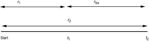
These dates are illustrated in Figure 4.6.
Figure 4.6 Key dates in a FRA trade.

The spot date is usually two business days after the trade date; however, it can by agreement be sooner or later than this. The settlement date will be the time period after the spot date referred to by FRA terms – for example, a 1×4 FRA will have a settlement date one calendar month after the spot date. The fixing date is usually two business days before the settlement date. The settlement sum is paid on the settlement date and, as it refers to an amount over a period of time that is paid upfront at the start of the contract period, the calculated sum is a discounted present value. This is because a normal payment of interest on a loan/deposit is paid at the end of the time period to which it relates. Because a FRA makes this payment at the start of the relevant period, the settlement amount is also a discounted present value sum.
With most FRA trades the reference rate is the LIBOR setting on the fixing date.
The settlement sum is calculated after the fixing date, for payment on the settlement date. We may illustrate this with a hypothetical example. Consider the case where a corporate has bought 1 million notional of a 1v4 FRA and dealt at 5.75%, and that the market rate is 6.50% on the fixing date. The contract period is 90 days. In the cash market the extra interest charge that the corporate would pay is a simple interest calculation:
![]()
The extra interest that the corporate is facing would be payable with the interest payment for the loan, which (as it is a money market loan) is when the loan matures. Under a FRA then, the settlement sum payable should be exactly equal to this if it was paid on the same day as the cash market interest charge. This would make it a perfect hedge. However, as we noted above, the FRA settlement value is paid at the start of the contract period – that is, at the beginning of the underlying loan and not the end. Therefore, the settlement sum has to be adjusted to account for this, and the amount of the adjustment is the value of the interest that would be earned if the unadjusted cash value was invested for the contract period in the money market. The settlement value is given by equation (4.1):
where
Equation (4.1) simply calculates the extra interest payable in the cash market, resulting from the difference between the two interest rates, and then discounts the amount because it is payable at the start of the period and not, as would happen in the cash market, at the end of the period.
In our hypothetical illustration, the corporate buyer of the FRA receives the settlement sum from the seller as the fixing rate is higher than the dealt rate. This then compensates the corporate for the higher borrowing costs that he would have to pay in the cash market. If the fixing rate had been lower than 5.75%, the buyer would pay the difference to the seller, because cash market rates will mean that he is subject to a lower interest rate in the cash market. What the FRA has done is hedge the interest rate, so that whatever happens in the market, it will pay 5.75% on its borrowing.
A market-maker in FRAs is trading short-term interest rates. The settlement sum is the value of the FRA. The concept is exactly the same as with trading short-term interest rate futures; a trader who buys a FRA is running a long position, so that if on the fixing date the settlement sum is positive and the trader realizes a profit. What has happened is that the trader, by buying the FRA, ‘borrowed’ money at an interest rate that subsequently rose. This is a gain, exactly like a short position in an interest rate future, where if the price goes down – that is, interest rates go up – the trader realizes a gain. Equally a ‘short’ position in a FRA, put on by selling a FRA, realizes a gain if on the fixing date.
FRA pricing
As their name makes clear, FRAs are forward rate instruments and are priced using standard forward rate principles.4 Consider an investor who has two alternatives: either a 6-month investment at 5% or a 1-year investment at 6%. If the investor wishes to invest for 6 months and then roll over the investment for a further 6 months, what rate is required for the rollover period such that the final return equals the 6% available from the 1-year investment? If we view a FRA rate as the breakeven forward rate between the two periods, we simply solve for this forward rate. The result is our approximate FRA rate.
We can use the standard forward rate breakeven formula to solve for the required FRA rate. The relationship given in equation (4.2) connects simple (bullet) interest rates for periods of time up to 1 year, where no compounding of interest is required. As FRAs are money market instruments we are not required to calculate rates for periods in excess of 1 year,5 where compounding would need to be built into the equation. The expression is:
where
![]()
This is illustrated diagrammatically in Figure 4.7.
Figure 4.7 Rates used in FRA pricing.
The time period is the time from the dealing date to the FRA settlement date, while is the time from the dealing date to the FRA maturity date. The time period for the FRA (contract period) is minus. We can replace the symbol ‘’ for time period with ‘’ for the actual number of days in the time periods themselves. If we do this and then rearrange the equation to solve for (the FRA rate) we obtain:
(4.3) ![]()
where
If the formula is applied to, say, US dollar money markets, the 365 in the equation is replaced by 360, the day-count base for that market.
In practice, FRAs are priced off the exchange-traded short-term interest rate future for that currency, so that sterling FRAs are priced off LIFFE short sterling futures. Traders normally use a spreadsheet pricing model that has futures prices directly fed into it. FRA positions are also usually hedged with other FRAs or short-term interest rate futures.
Interest rate swaps
An interest rate swap is an off-balance-sheet agreement between two parties to make periodic interest payments to each other. Payments are on a predetermined set of dates in the future, based on a notional principal amount; one party is the fixed rate payer, the rate agreed at the start of the swap, and the other party is the floating rate payer, the floating rate being determined during the life of the swap by reference to a specific market rate or index. There is no exchange of principal, only of the interest payments on this principal amount. Note that our description is for a plain vanilla swap contract; it is common to have variations on this theme – for instance, floating–floating swaps where both payments are floating rate, as well as cross-currency swaps where there is an exchange of an equal amount of different currencies at the start dates and end dates of the swap.
An interest rate swap can be used to hedge the fixed rate risk arising from originating a loan at a fixed interest rate, such as a fixed rate mortgage. The terms of the swap should match the payment dates and maturity date of the loan. The idea is to match the cashflows from the loan with equal and opposite payments in the swap contract, which will hedge the mortgage position. For example, if the retail bank has advanced a fixed rate mortgage, it will be receiving fixed rate coupon payments on the nominal value of the loan (together with a portion of the capital repayment if it is a repayment mortgage and not an interest-only mortgage). To hedge this position the trader buys a swap contract for the same nominal value in which he will be paying the same fixed rate payment; net cashflow is a receipt of floating interest rate payments.
A borrower, on the other hand, may issue bonds of a particular type because of investor demand for such paper, but prefer to have the interest exposure on the debt in some other form. So, for example, a UK company issues fixed rate bonds denominated in, say, Australian dollars, swaps the proceeds into sterling and pays floating rate interest on the sterling amount. As part of the swap the company will be receiving fixed rate Australian dollars which neutralizes the exposure arising from the bond issue. On termination of the swap (which must coincide with the maturity of the bond) the original currency amounts are exchanged back, enabling the issuer to redeem the holders of the bond in Australian dollars.
For detailed coverage of interest rate swaps and their application see Choudhry (2007).
Description
Swaps are derivative contracts involving combinations of two or more interest rate bases or other building blocks. Most swaps currently traded in the market involve combinations of cash market securities – for example, a fixed interest rate security combined with a floating interest rate security, possibly also combined with a currency transaction. However, the market has also seen swaps that involve a futures or forward component, as well as swaps that involve an option component. The market for swaps is organized by the International Swaps and Derivatives Association (ISDA).
Example 4.5 Comparative advantage and interest rate swap structure
When entering into a swap either for hedging purposes or to alter the basis of an interest rate liability, the opposite of a current cashflow profile is required. Consider a homeowner with a variable rate mortgage. The homeowner is at risk from an upward move in interest rates, which will result in her being charged higher interest payments. She wishes to protect herself against such a move and in theory (Don’t try this with your building society!), as she is paying floating, she must receive floating in a swap. Therefore, she will pay fixed in the swap. The floating interest payments cancel each other out, and the homeowner now has a fixed rate liability. The same applies in a hedging transaction: a bondholder receiving fixed coupons from the bond issuer – that is, the bondholder is a lender of funds – can hedge against a rise in interest rates that lowers the price of the bond by paying fixed in a swap with the same basis point value as the bond position; the bondholder receives floating interest. Paying fixed in a swap is conceptually the same as being a borrower of funds; this borrowing is the opposite of a loan of funds to the bond issuer and therefore the position is hedged. Consider two companies’ borrowing costs for a 5-year loan of 50 million:
- Company A can pay fixed at 8.75% or floating at Libor. Its desired basis is floating.
- Company B can pay fixed at 10% or floating at Libor100 basis points. Its desired basis is fixed.
Without a swap:
Company A borrows fixed and pays 8.75%;
Company B borrows floating and pays Libor100 basis points.
Let us say that the two companies decide to enter into a swap, whereby Company A borrows floating rate interest and therefore receives fixed from Company B at the 5-year swap rate of 8.90%. Company B, which has borrowed at Libor100 basis points, pays fixed and receives Libor in the swap. Company A ends up paying floating rate interest, and company B ends up paying fixed.
The result after the swap:
![]()
Company A saves 15 basis points (pays L15bp rather than L flat) and B saves 10 basis points (pays 9.90% rather than 10%).
Both parties benefit from the comparative advantage of A in the fixed rate market and B in the floating rate market (spread of B over A is 125bp in the fixed rate market but 100bp in the floating rate market). Originally swap banks were simply brokers, and charged a fee to both counterparties for bringing them together. In the example Company A deals direct with Company B, although it is more likely that an intermediary bank would have been involved.
As the market developed, banks became principals and dealt direct with counterparties, eliminating the need to find someone who had requirements that could be met by the other side of an existing requirement.
An interest rate swap is an agreement between two counterparties to make periodic interest payments to one another during the life of the swap, on a predetermined set of dates, based on a notional principal amount. One party is the fixed rate payer, and this rate is agreed at the time of trade of the swap; the other party is the floating rate payer, the floating rate being determined during the life of the swap by reference to a specific market index. The principal or notional amount is never physically exchanged, hence the term ‘off balance sheet’, but is used to calculate interest payments. The fixed rate payer receives floating rate interest and is said to be ‘long’ or to have ‘bought’ the swap. The long side has conceptually purchased a floating rate note (because it receives floating rate interest) and issued a fixed coupon bond (because it pays out fixed interest at intervals) – that is, it has in principle borrowed funds. The floating rate payer is said to be ‘short’ or to have ‘sold’ the swap. The short side has conceptually purchased a coupon bond (because it receives fixed rate interest) and issued a floating rate note (because it pays floating rate interest).
So, an interest rate swap is
an agreement between two parties to exchange a stream of cashflows calculated as a percentage of a notional sum and on different interest bases.
For example, in a trade between Bank A and Bank B, Bank A may agree to pay fixed semi-annual coupons of 10% on a notional principal sum of 1 million, in return for receiving from Bank B the prevailing 6-month sterling Libor rate on the same amount. The known cashflow is the fixed payment of 50,000 every 6 months by Bank A to Bank B.
Like other financial instruments, interest rate swaps trade in a secondary market. The value of a swap moves in line with market interest rates, in exactly the same fashion as bonds. If a 5-year interest rate swap is transacted today at a rate of 5% and 5-year interest rates fall to 4.75% shortly thereafter, the swap will have decreased in value to the fixed rate payer, and correspondingly increased in value to the floating rate payer, who has now seen the level of interest payments fall. The opposite would be true if 5-year rates moved to 5.25%. Why is this? Consider the fixed rate payer in an IR swap to be a borrower of funds. If she fixes the interest rate payable on a loan for 5 years and then this interest rate decreases shortly afterwards, is she better off? No, because she is now paying above the market rate for the funds borrowed. For this reason a swap contract decreases in value to the fixed rate payer if there is a fall in rates. Equally, a floating rate payer gains if there is a fall in rates, as he can take advantage of the new rates and pay a lower level of interest; hence, the value of a swap increases to the floating rate payer if there is a fall in rates.
The P&L profile of a swap position is shown in Table 4.2.
Table 4.2 Impact of interest-rate changes.
| Fall in rates | Rise in rates | |
| Fixed rate payer | Loss | Profit |
| Floating rate payer | Profit | Loss |
Example of vanilla interest rate swap
The following swap cashflows are for a ‘pay fixed, receive floating’ interest rate swap with the following terms:
| Trade date | 3 December 2010 |
| Effective date | 7 December 2010 |
| Maturity date | 7 December 2015 |
| Interpolation method | Linear |
| Day-count (fixed) | Semi-annual, act/365 |
| Day-count (floating) | Semi-annual, act/365 |
| Nominal amount | 10 million |
| Term | 5 years |
| Fixed rate | 4.73% |
The interest payment dates of the swap fall on 7 June and 7 December; the coupon dates of benchmark gilts also fall on these dates, so even though the swap has been traded for conventional dates, it is safe to surmise that it was put on as a hedge against a long gilt position. Fixed rate payments are not always the same, because the actual/365 basis will calculate slightly different amounts.
The swap we have described is a plain vanilla swap, which means it has one fixed rate and one floating rate leg. The floating interest rate is set just before the relevant interest period and is paid at the end of the period. Note that both legs have identical interest dates and day-count bases, and the term to maturity of the swap is exactly 5 years. It is of course possible to ask for a swap quote where any of these terms have been set to customer requirements; for example, both legs may be floating rate, or the notional principal may vary during the life of the swap. Non-vanilla interest rate swaps are very common, and banks will readily price swaps where the terms have been set to meet specific requirements. The most common variations are different interest payment dates for the fixed rate leg and floating rate leg, on different day-count bases, as well as terms to maturity that are not whole years.
Swap spreads and the swap yield curve
In the market, banks will quote two-way swap rates – on screens, on the telephone or via a dealing system such as Reuters. Brokers will also be active in relaying prices in the market. The convention in the market is for the swap market-maker to set the floating leg at Libor and then quote the fixed rate that is payable for that maturity. So, for a 5-year swap a bank’s swap desk might be willing to quote the following:
| Floating rate payer: | pay 6-month Libor receive fixed rate of 5.19% |
| Fixed rate payer: | pay fixed rate of 5.25% receive 6-month Libor |
In this case the bank is quoting an offer rate of 5.25%, which the fixed rate payer will pay in return for receiving Libor flat. The bid price quote is 5.19% which is what a floating rate payer will receive fixed. The bid–offer spread in this case is therefore 6 basis points. Fixed rate quotes are always at a spread above the government bond yield curve. Let us assume that the 5-year gilt yields 4.88%; in this case, then, the 5-year swap bid rate is 31 basis points above this yield. So, the bank’s swap trader could quote swap rates as a spread above the benchmark bond yield curve, say 37-31, which is her swap spread quote. This means that the bank is happy to enter into a swap paying fixed 31 basis points above the benchmark yield and receiving Libor, and receiving fixed 37 basis points above the yield curve and paying Libor. The bank’s screen on, say, Bloomberg or Reuters might look something like Table 4.3, which quotes swap rates as well as the current spread over the government bond benchmark.
Table 4.3 Swap quotes.
A swap spread is a function of the same factors that influence the spread over government bonds for other instruments. For shorter duration swaps – say, up to 3 years – there are other yield curves that can be used in comparison, such as the cash market curve or a curve derived from futures prices. For longer dated swaps the spread is determined mainly by the credit spreads that prevail in the corporate bond market. Because a swap is viewed as a package of long and short positions in fixed rate and floating rate bonds, it is the credit spreads in these two markets that will determine the swap spread. This is logical; essentially, it is the premium for greater credit risk involved in lending to corporates that dictates that a swap rate will be higher than same maturity government bond yield. Technical factors will be responsible for day-to-day fluctuations in swap rates, such as the supply of corporate bonds and the level of demand for swaps, plus the cost to swap traders of hedging their swap positions.
Overnight interest rate swaps
An interest rate swap contract, which is generally regarded as a capital market instrument, is an agreement between two counterparties to exchange a fixed interest rate payment in return for a floating interest rate payment, calculated on a notional swap amount, at regular intervals during the life of the swap. A swap may be viewed as being equivalent to a series of successive FRA contracts, with each FRA starting as the previous one matures. The basis of the floating interest rate is agreed as part of the contract terms at the inception of the trade. Conventional swaps index the floating interest rate to Libor; however, an exciting recent development in the sterling money market has been the sterling overnight interest rate average or SONIA. In this section we review SONIA swaps, which are extensively used by sterling market banks.
SONIA is the average interest rate of interbank (unsecured) overnight sterling deposit trades undertaken before 15:30 hours each day between members of the London Wholesale Money Brokers’ Association. Recorded interest rates are weighted by volume. A SONIA swap is a swap contract that exchanges a fixed interest rate (the swap rate) against the geometric average of overnight interest rates that have been recorded during the life of the contract. Exchange of interest takes place on maturity of the swap. SONIA swaps are used to speculate on or to hedge against interest rates at the very short end of the sterling yield curve; in other words, they can be used to hedge an exposure to overnight interest rates.6 The swaps themselves are traded in maturities of 1 week to 1 year, although 2-year SONIA swaps have also been traded.
Conventional swap rates are calculated off the government bond yield curve and represent the credit premium over government yields of interbank default risk. In essence, they represent average forward rates derived from the government spot (zero-coupon) yield curve. The fixed rate quoted on a SONIA swap represents the average level of overnight interest rates expected by market participants over the life of the swap. In practice, the rate is calculated as a function of the Bank of England’s repo rate. This is the 2-week rate at which the Bank conducts reverse repo trades with banking counterparties as part of its open market operations. In other words, this is the Bank’s base rate. In theory, we would expect the SONIA rate to follow the repo rate fairly closely, since the credit risk on an overnight deposit is low. However, in practice, the spread between the SONIA rate and the Bank repo rate is very volatile, and for this reason the swaps are used to hedge overnight exposures.
Example 4.6 Using an OIS swap to hedge a funding requirement
A structured hedge fund derivatives desk at an investment bank offers a leveraged investment product to a client in the form of a participating interest share in a fund of hedge funds. The client’s investment is made up partly of funds lent to it by the investment bank, for which the interest rate charged is overnight Libor (plus a spread).
This investment product has an expected life of at least 2 years. As part of its routine asset–liability management operations, the bank’s Treasury desk has been funding this requirement by borrowing overnight each day. It now wishes to match the funding requirement raised by this product by matching the asset term structure to the liability term structure. Let us assume that this product creates a USD1 billion funding requirement for the bank.
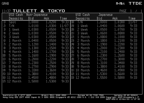
Current market depo rates are shown in Figure 4.8. The Treasury desk therefore funds this requirement in the following way:
Figure 4.8 Illustration of interest basis mismatch hedging using the OIS instrument.
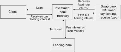
This matches the asset structure more closely to the term structure of assets; however, it opens up an interest rate basis mismatch in that the bank is now receiving an overnight Libor-based income but paying a term-based liability. To remove this basis mismatch, the Treasury desk transacts an OIS swap to match the amount and term of each of the loan deals, paying overnight floating rate interest and receiving fixed rate interest. The rates for OIS swaps of varying terms are shown in Figure 4.9, which shows two-way prices for OIS swaps up to 2 years in maturity. So, for the 6-month OIS the hedger is receiving fixed interest at a rate of 1.085% and for the 12-month OIS he is receiving 1.40%. The difference between what he is receiving in the swap and what he is paying in term loans is the cost of removing the basis mismatch, but more fundamentally reflects a key feature of OIS swaps versus deposit rates: depo rates are Libor-related, whereas US dollar OIS rates are driven by the Fed Funds rate. On average, the Fed Funds rate lies approximately 8–10 basis points below the dollar deposit rate, and sometimes as much as 15 basis points below cash levels.
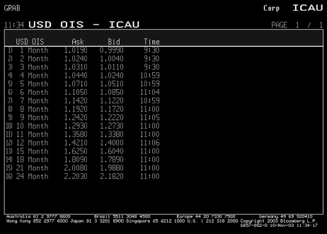
Figure 4.9 Tullet US dollar depo rates, 10 November 2003.
This action hedges out the basis mismatch and also enables the Treasury desk to match its asset profile with its liability profile. The net cost to the Treasury desk represents its hedging costs.
Figure 4.10 illustrates the transaction.
Figure 4.10 Garban ICAP OIS rates for USD, 10 November 2003.
Example 4.9 Cashflows on OIS
Table 4.4 shows daily rate fixes on a 6-month OIS that was traded for an effective date of 17 October 2003, at a fixed rate of 1.03%. The swap notional is USD200 million.
From Table 4.4 we see that the average rate for Fed Funds during this period was 0.99952%. Hence, on settlement the fixed rate payer would have passed over a net settlement amount of USD30,480.
Table 4.4 OIS cash flows.
CREDIT RISK HEDGING
The business of banking – lending money to and trading with counterparties who carry default risk – creates credit risk exposure on the bank’s balance sheet. This must be managed actively. In many cases, once a loan is originated, it cannot be removed from the balance sheet, so the act of risk management involves raising the capital base of the bank in anticipation of a deterioration in general economic conditions. Equally, the bank might raise its loan origination standards, and reduce the amount it lends to borrowers of lower credit quality.
The other side of the approach to credit risk management is to sell loans where possible, to remove them from the balance sheet via securitization or to use credit derivatives. This topic is covered in detail in Choudhry (2007).
Understanding credit risk
Credit risk management is a judgement call. The one single factor that most assists effective credit risk management is knowing one’s market. Unfamiliarity with a particular market or customer set, or over-reliance on ‘black box’ models to assess loan origination quality, hampers the application of credit risk, because it renders it susceptible to the business cycle. So, beyond understanding the drivers of credit risk and their dynamics, the over-riding principle remains to understand the market we are operating in. Never originate loans or invest in assets that we do not understand. This principle does not change irrespective of the level of sophistication of the product or customer. In other words, the complexity of a product or transaction does not alter the requirement to understand the borrower and its business risks. That is what credit risk is. Even with sophisticated transactions or complex products, while the evaluation of the risk exposure may be more difficult, the need to understand the nature of the risk does not alter. Ultimately, the question of credit risk management remains the same: What is the chance that the investment will incur losses, and how much will the lender lose if the borrower is unable to repay? The answer to this question, which is dynamic, guides the approach to bank credit risk management.
Definition of credit risk
Credit risk is the risk of loss due to a ‘credit event’. This was the case before the advent of the credit derivative market which placed this term into regular usage. A credit event can be a number of things, from outright default due to bankruptcy, liquidation or administration, or it can be something short of full default. It can also mean loss due to credit migration, such as a downgrade in credit rating. In the credit derivatives market, the range of credit events is defined in the legal documentation governing the market. In a full default, the extent of loss can be observed immediately to be the full notional amount of the loan; however, over time, the lender will typically receive an amount of the loan back from the administrators, known as the ‘recovery value’. In a credit loss event short of default, the amount of loss is determined by applying mark-to-market (MtM) valuation.
Default itself is defined in more than one way. Generally, it is one or more of the following:
- non-payment of interest 90 days after the interest due date;
- non-payment of a loan 90 days after the loan maturity date;
- restructuring of the borrower’s loans;
- filing for bankruptcy, the appointment of administrators, liquidation, and so on.
Late payment is often termed a non-performing loan (NPL) or a delinquent loan rather than a defaulted loan if the borrower is still undertaking business. However, at some point, irrespective of the state of the borrower, an NPL will be written off as a default loss. The write-down, which must be funded out of the bank’s capital, is often at 100% of outstanding notional value, even though the bank will probably recover a percentage, however small, at some later date. Another definition of default is that presented by Merton in his 1974 paper. This states that default occurs when the value of a company falls below the value of its debts. The definition of default is relevant because for some models it is a driver of the calculation of default probability; it is also relevant to credit rating agencies when they compile the historical frequency of default. Rating agencies generally apply the delay-in-payment definition.
Asset exposure
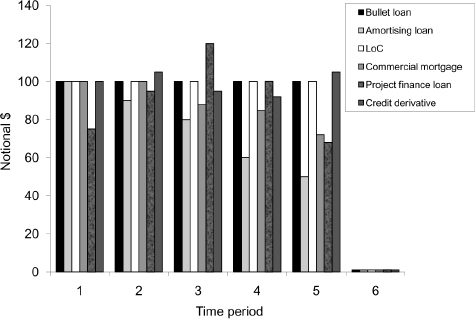
The notional, or absolute, level of risk exposure is the first port of call. It is also the easiest to calculate. It is given by the amount of the loan or investment with the customer or ‘counterparty’.7 This amount may be fixed, sometimes called a ‘bullet’ loan, or it may reduce steadily, which is an amortising loan. If the exposure is a vanilla loan that is recorded in the bank’s balance sheet, the amount will not change from the origination date to the maturity date. If it is a loan that is tradeable, such as a bond, or otherwise subject to MtM valuation, then the exposure amount will vary according to its valuation, but should always be 100% of notional by the maturity date. Figure 4.11 is a stylized representation of the behaviour of asset risk exposure by type of asset, each of which has the same maturity date.8
Figure 4.11 Notional value risk exposure profiles of different product types
Trading book assets apply MtM. The value of a loan that is under MtM will change because of changes to the general level of interest rates, and/or changes to the credit standing of the borrower (or the borrower’s industrial sector, or to credit conditions generally in the market). As such, trading book assets capture changes in value, at least theoretically, that arise due to, for instance, changes in credit rating. This is known as credit migration risk. The banking book, which does not apply MtM, cannot by definition capture the migration risk of its assets. It only captures the risk of loss due to default. This might be seen to be some sort of disadvantage, because changes in the credit standing of a borrower also change its probability of default. However, use of MtM in a trading book is less of an advantage than we might think, and in stressed market conditions it can be self-defeating (lower MtM values can generate a vicious circle of falling prices that impacts confidence and can itself lead to default).
Asset exposure on a balance sheet is not comprised solely of live loans. It also includes potential future liabilities, such as letters of credit, third-party liquidity lines and other guarantees. The notional amount of such off-balance-sheet exposures is also part of the bank’s credit risk exposure.
The main risk management mechanism for asset exposure risk is by means of credit limits. This is the maximum amount that can be outstanding at any time to the individual customer, the industrial sector, the country, and so on. Limits can also be set by currency.
Credit rating rationale
Lenders and investors use a credit rating, often alphanumeric, to describe the credit risk of an obligor. They represent, either implicitly or explicitly, a default probability of the borrower over a specified time period. The ratings used can be those of an external agency or those internal to the bank. The Basel II regulatory capital methodology makes use of either formal external ratings, in its standardized approach, or of bank internal ratings, in its internal ratings-based approach.
The credit rating process for corporates applies a number of qualitative and quantitative factors, which we describe below. For SPV-type companies a quantitative approach can only be used, and therefore is used. A bank’s internal ratings system uses the same sort of approach, making use of default probabilities and recovery rates.
Bank internal credit ratings
All banks employ some form of internal credit rating methodology for their customers. The rating criteria for bank internal systems are similar in concept to those of external agencies; that is, they include qualitative and quantitative factors. Criteria are tweaked in accordance with the type of borrower being assessed. For example, financial institutions will be assessed by bank-specific metrics such as the loan-to-deposit ratio or the level of loan loss reserves.
In recent years there has been a tendency for banks to adopt a ‘black box’ approach, in which loan agents input the required parameters into their system and model output either approved or disapproved the loan. A reduced level of human judgement in the loan origination process has limitations that are exposed during a recession or economic crash, mainly because black box models are not immune to being sucked into a bull market. For this reason, it is important that the loan approval process includes an element of operator judgement, which is of value when the operator is familiar with the market.
Internal ratings are similar to external ones in assigning an alphanumeric grade to borrowers that ranks their credit standing. For many banks, the customers in question will be small-and-medium-sized enterprises (SMEs) and so will not possess an external agency credit rating. For SMEs it is mainly the internal bank rating that will drive the loan approval process. A bank’s credit analysis department will consider the obligor’s risk of default, the credit quality of any parent or supporting company, the risk of the loan product itself and the backing of any other banking institution when calculating its internal rating. Assessment of the borrower’s risk of default is similar to the qualitative and financial review used by external agencies.
A bank operating across more than one legal jurisdiction will also want to have an internal rating for each country. This is important because, depending on the country concerned, it may be difficult or impossible to recover cash or assets in the event of default or to enforce a legal ruling. Therefore, a foreign country rating is required as well. This remains important even if the obligor is rated higher than its domicile country, because of the potential legal problems just noted.
The Basel II rules crystallized the use of credit ratings by making explicit reference to them in its standardized approach (see Chapter 10). However, for many banks the standardized approach is no less risk insensitive than Basel I, because their customers are not externally rated. Such banks can map external ratings to their internal system and assign risk weights accordingly, providing they have obtained regulator approval for their internal model. Generally, this mapping process involves applying external ratings and their implied default probabilities to the internal rating and obtaining an external rating equivalent to the internal grade. This can be undertaken using an off-the-shelf credit model. Although this process is in common use, it is inherently flawed because of its reliance on the two usual parameters: default probability and recovery rate (RR). The rating criteria reflect the ‘expected loss’ (EL) of an asset, given by
![]()
We see then that EL can alter significantly by changing RR, even if default probability stays unchanged. This in turn can change the external rating. Table 4.5 shows Moody’s statistics for ratings and default, and the equivalent for each rating grade. It is possible to alter a ratings-equivalent default rate by changing the recovery rate, and thereby obtain a different rating. Business best practice and prudent risk management dictate, therefore, that banks assume a 0% recovery rate in their internal ratings systems.
Table 4.5 Moody’s rating statistics 2007.
| Rating | Yearly average default rate (%) | Yearly volatility of default rate (19702007) (%) |
| Aaa | 0.00 | 0.00 |
| Aa | 0.05 | 0.12 |
| A | 0.08 | 0.05 |
| Baa | 0.20 | 0.29 |
| Ba | 1.80 | 1.40 |
| B | 8.30 | 5.03 |
| Source: Moody’s Inc., reproduced with permission | ||
Credit limit setting and rationale
For many commercial banks, and certainly all smaller banks, credit limits and credit exposure on a day-to-day basis are perhaps the most important aspects of the risk management process, given that such institutions should not be running much market risk. The latter is more of an issue for larger banks, multinational banks and market-making banks. While liquidity risk management is universal to all banks, maintaining effective credit risk origination standards and a limit-setting policy is essential for the vast majority of banks that do not carry material market risk. Smaller banks are less likely to be rescued by the central bank or the government if they fail, because they would not be deemed ‘systemically important’, so a prudent credit risk management culture and through-the-cycle macroprudential procedures are of primary importance for such firms.9
We now discuss the business best practice principles of credit limit setting and the loan origination process.
Credit process
Banks generally operate one of two types of approval process: (i) via a credit committee or (ii) via delegated authority from the credit committee to a business line head. The committee process is designed to ensure that there is proper scrutiny of any transaction that commits the bank’s capital. The sponsor bringing the transaction to the committee is the front office business line; the committee will approve or decline based on the risk–reward profile of the transaction.
Procedure (ii) is common for high-volume business, for which the committee process as a consequence of it being time consuming would not be practical. As we note above, there is uncertainty that the ‘know your risk’ principle can be diluted, particularly in a competitive environment where a bank is trying to build volume. Given this uncertainty, ‘market share’ should not be a performance indicator, or target, for a bank’s business line. Rather, performance should be measured only via the amount of genuine shareholder value added that the business generates.
Credit limit principles
The point of credit risk limits is to set an upper bound to the loss that can be suffered by a bank at any one time.
The basic principles of credit limit setting are universal for every bank and follow the essential requirements of prudence and concentration. In other words, an element of diversification in the loan portfolio is necessary, although at all times the bank should practice the basic principle of ‘know your risk’. In other words, diversity as an end in itself is not recommended good practice; a bank should diversify only into sectors that it thoroughly understands and in which it has some competitive advantage or valuable skill base.
In standard textbooks on finance and banking, we read that it is the capital base that drives the limit-setting process. Essentially, what this is saying in practice is that we take the amount of capital available and allocate it as per credit limit buckets for each of the businesses. Actually, the proper and intellectually robust way to do this is the other way around: the bank should determine its strategy and business model, as well as preparing budgets based on the risk exposure that it considers it has the expertise to manage. This process then drives the level of capital and regulatory capital that the bank should then set up. Once this amount is known and achieved, it can then be allocated to specific business lines as lower level credit limits by geography, industry, product and so on.
The essential principles governing limit setting include the following:
- All single exposures should be sufficiently contained such that a complete default, running the risk of 0% recovery, can be contained within the existing capital base and does not endanger the bank as a going concern. In other words, after the loss the bank should still be within its regulatory capital limits.
- The loan portfolio should be diversified by industrial sector, geography and product line, within the knowledge base and expertise of the bank.
- Set minimum internal (and, if desired, external) rating criteria below which the bank will not lend. For example, this may be ‘investment grade rated only’ or ‘no lending to entities with an internal rating equivalent to BB/Ba2’.
- Do not lend to obligors any amount that as a result overextends them and creates a situation in which repayment is put at risk. This requires that the ‘know your risk’ dictum be applied equally to understanding the customer’s risks. This should be assessed via an analysis of the borrower’s financial indicators, including leverage ratio, debt service coverage ratio, and so on.
- Set limit categories to avoid concentration, and also by borrower rating.
As part of a transaction origination process, reviewers must consider what ‘ancillary business’ can be generated from the same borrower. The bank must set a policy that dictates how much this ancillary business drives the origination process, whether the lending business can be a ‘loss leader’ to an extent or can create sufficient shareholder value added in its own right.
Credit limit setting
The process of setting credit limits is very important to all banks – vanilla commercial banks, in particular – in so far as credit risk exposure generates the highest losses for such institutions. The process should follow prudent and robust policy and be run according to cycle-proof principles to avoid getting overextended during a bull market, when loan origination standards are relaxed. Credit limits are set for a range of criteria, which are deliberately set as overlapping so as to ensure that all the various different categories of risk exposure are captured.
Macro-level credit limits are set per individual obligor, originated within the business lines but approved by the Executive Credit Committee and secondarily approved by ALCO. When necessary, if the size of a transaction dictates it, further approval may be needed by the Executive Management Committee (ExCo) and the board itself. The level of capital allocation required for a particular limit application determines how far up the governance structure it needs to go. Formal limits on capital allocation are therefore set at ExCo approval level.
The limit-setting process is designed to produce overlapping limits. Limits will be set in the following categories:
- Individual obligor. This is further split into limit by product class, limit globally and limit locally. Sub-limits do not necessarily aggregate to the overall obligor limit: this is to prevent excess exposure in one product class or geographical region. Sub-limits are also set per currency. At all times, the obligor’s exposure cannot exceed its overall limit.
- Geographical region. This is further split into country limits and individual regions within a country.
- Industrial sector.
As no individual limit can be breached, any new capital-using transaction must fit into the capacity allowed by all three limit categories.
Limit excess is a serious breach of management governance and must be reported to ALCO (and, if necessary, ExCo) for corrective action. This can be one or more of the following: (i) cease further business with the specific obligor; (ii) transfer some of the exposure, either by secondary market sale, securitization, or hedging with credit derivatives; (iii) increase the limit; (iv) transfer some capacity from another part of the business and/or another obligor.
Loan origination process standards
The loan origination process differs across banks. The detail of an individual specific process is not of major interest to us. What is important is that this origination process adheres to basic principles of prudence, and that these are controlled and managed to ensure they are ‘through the cycle’; that is, a reduction in standards, or a relaxation of them during a period of economic growth, is something that should require board approval. Enlarging the balance sheet during a bull market is a risky strategy, because it is during this time that standards are lowered and low-quality and/or underpriced assets are put on the book.
An example of this occurred at the failed UK banks Northern Rock and Bradford & Bingley, which originated large numbers of 100LTV and 125LTV mortgages, as well as more risky buy-to-let mortgages. The failed bank HBOS (in common with many banks at the time) operated a loan origination process for retail and corporate loans that delegated the approval decision to a black box computer model, which rated all applications in a tick box process that assigned a credit score and then approved on that basis. This is understandable for high-volume business models, but sacrifices a large element of ‘know your customer’ in the approval process.
The essential guidelines for a through-the-cycle asset origination standards process include:
- Know your customer. For one-off and/or big-ticket transactions this principle is straightforward to apply. It is more difficult for large-volume business, particularly when the bank has adopted a black box system in which approval is granted by a model (the applicant’s details are input to the system and the system generates the approval without any loan officer or credit expert reviewing the application). This is common practice for retail business such as credit card and mortgage applications, especially for business conducted over the telephone or internet. The danger is that, in a commoditized and competitive market, origination standards are lowered and the bank creates a pool of lower quality assets, the obligors for which it is not familiar with and whose financial strength it cannot be certain of. This was an acute problem for retail mortgage banks in the US, UK, Ireland and Spain (amongst others) during 2002–2007, all of whom experienced a housing boom and bust in this period. Business best practice dictates that for all origination business, banks must know their customer base at all times (see below on mortgages). This means that the black box application process must be supplemented with a review by an experienced loan analyst.
- Loan security. The collateral acceptable for a loan should at all times be of sufficient liquidity and value. The bank must be able to realize the collateral if the obligor defaults. Genuine liquidity through all market conditions is restricted to sovereign liabilities only, so to cover for the loss of liquidity in other types of collateral, the bank must ensure sufficient margin over and above the loan value.
- Subprime-lending restrictions. Assets against which no collateral or insufficient collateral is taken should at all times be subject to restrictions and severe limits because these types of assets are the first to experience default when the economy experiences a downturn. Mortgages that are not covered by sufficient collateral, such as 100LTV or 125LTV loans where the advance is greater than the value of the security, and other subprime mortgages or higher risk mortgages such as ‘self-certified’ loans should similarly be subject to restriction.
Excluding the peak of an overheating economy just about to enter a recession, loan defaults typically do not occur at the start or end of a loan’s term. Another exception is right at the end of a bull market, when bank loan origination standards have been lowered and asset prices (credit spreads) are at their most undervalued, when banks write much low-quality business. Leaving that aside, the most common time of default is generally between 45 and 55 months after the loan start date. This means that default statistics considerably lag the actual state of the economy. Given historical default rates, which banks use to assist them in setting their credit limits, there is a danger that business continues to be written at lower credit standards at the time when the bank should be reigning in risky business. This is why the basic principles we summarize above should be observed at all times; they should act as a guiding light for a bank’s Executive Credit Committee.
BIBLIOGRAPHY
Choudhry, M. (2007) Bank Asset and Liability Management, John Wiley Asia.
Cox, J., Ingersoll, J., and Ross, S. (1981) ‘The Relationship between Forward Prices and Futures Prices,’ Journal of Financial Economics, 9, December, 321–346.
Fabozzi, F. and Mann, S. (2001) Introduction to Fixed Income Analytics, FJF Associates, Chapter 2.
French, K. (1983) ‘A Comparison of Futures and Forwards Prices,’ Journal of Financial Economics, 12, November, 311–342.
Hull, J. (1999) Options, Futures and Other Derivatives, Fourth Edition, Prentice-Hall.
Jarrow, R. and Oldfield, G. (1981) ‘F#orward Contracts and Futures Contracts,’ Journal of Financial Economics, 9, December, 373?–382.
Kimber, A. (2004) Credit Risk, Oxford: Elsevier.
Merton, R.C. (1974) ‘On the pricing of corporate debt: The risk structure of interest rates,’ Journal of Finance, 29(2), May, 449–470.
Rubinstein, M. (1999) Rubinstein on Derivatives, RISK Publishing, Chapter 2.
Windas, T. (1993) An Introduction to Option-Adjusted Spread Analysis, Bloomberg Publishing, Chapter 3
1 See Choudhry (2007).
2 A repo dealer is a market-maker, and so offers stock in repo at the offered side, which is 5.75%. However, this trade still turns in a profit if the bank dealt at another market-maker’s bid side of 5.83%, with a profit of 9 basis points on the cash sum. Rates are quoted from King & Shaxson Bond Brokers Limited.
3 Thanks to Del Boy at King & Shaxson Bond Brokers Ltd for pointing this out, although I still reckon that my definition is the right one!
4 An introduction to the basics of spot and forward rates can be found in any number of finance textbooks; the author particularly likes Windas (1993) and Fabozzi and Mann (2001), both of which are highly suitable for beginners.
5 Although it is of course possible to trade FRAs with contract periods greater than 1 year, for which a different pricing formula must be used.
6 Traditionally, overnight rates fluctuate widely during the day, depending on the day’s funds shortage, and although volatility has reduced since the introduction of gilt repo it is still unpredictable on occasion.
7 We have to be careful with the use of the word ‘investment’. Here we mean investment from the viewpoint of the bank. In general conversation, investment is often used to mean an equity investment by a shareholder in the business. If a bank advances debt funds to a customer, this is of course also an investment in the future wellbeing of the company.
8 This is for illustration. It is highly uncommon to observe such a different range of asset types with identical maturity dates. Mortgage and project finance loans have the longest legal final maturity dates.
9 In the US alone, according to the FDIC website, there were 25 bank failures in 2008, 140 in 2009 and 157 in 2010. This compares with just 11 bank failures during the period 2003–2007. With the exception of Washington Mutual Bank, these failing banks did not make the media headlines, due to their small size and domestic business base; nevertheless, a failed bank in any jurisdiction and of any size is a gross failure of management and corporate governance. Regulatory authorities should have the objective of treating all banks as systemically important.