Search in book...
Toggle Font Controls
Create new playlist

Name your new playlist

Playlist description (optional)
Sign In

Email address

Password

Forgot Password?

or

Continue with Facebook

Continue with Google
Sign Up

Full Name

Email address

Confirm Email Address

Password

or

Continue with Facebook

Continue with Google

Chapter 6
INTRODUCTION TO MONEY MARKET DEALING AND HEDGING

In this chapter we introduce some basics of trading and hedging as employed by a bank asset–liability management (ALM) or money market desk. The instruments and techniques used form the fundamental building blocks of ALM, so the reader can imagine that a full and comprehensive treatment of this subject would require a book in its own right.¹ Our purpose here is to acquaint the newcomer to the market with the essentials. The market yield curve and the bank's internal curve are paramount in this discipline, which is why we introduced that topic earlier. The next two chapters look at the ALM discipline in more detail.

The ALM and money market desk has a vital function in a bank, funding all the business lines in the bank. In some banks and securities houses it will be placed within the Treasury or money market areas, whereas other firms will organise it as an entirely separate function. Wherever it is organised, the need for clear and constant communication between the ALM desk and the other operating areas of the bank is paramount. But first we look at specific uses of money market products like deposits and repo in the context of the shape of the yield curve.

MONEY MARKET APPROACH

The yield curve and interest‐rate expectations

When the yield curve is positively sloped, the conventional approach is to fund the book at the short end of the curve and lend at the long end. In essence, therefore, if the yield curve resembled that shown in Figure 6.1, a bank would borrow, say, 1‐week funds while simultaneously lending out at, say, 3‐month maturity. This is known as funding short. A bank can effect the economic equivalent of borrowing at the short end of the yield curve and lending at the longer end through repo transactions – in our example, a 1‐week repo and a 6‐month reverse repo. The bank then continuously rolls over its funding at 1‐week intervals for the 6‐month period. This is also known as creating a tail; here the “tail” is the gap between 1 week and 6 months – the interest‐rate “gap” that the bank is exposed to. During the course of the trade – as the reverse repo has locked in a loan for 6 months – the bank is exposed to interest‐rate risk should the slope or shape of the yield curve change. In this case, the bank may see its profit margin shrink or turn into a funding loss if short‐dated interest rates rise.

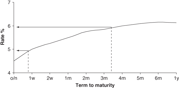
Graphical illustration of a positive yield curve funding. — *Figure 6.1* Positive yield curve funding

As we noted in Chapter 5, a number of hypotheses have been advanced to explain the shape of the yield curve at any particular time. A steep positive‐ shaped curve may indicate that the market expects interest rates to rise over the longer term, although this is also sometimes given as the reason for an inverted curve with regard to shorter term rates. Generally speaking, trading volumes are higher in a positive‐sloping yield curve environment, compared with a flat or negative‐shaped curve.

In the case of an inverted yield curve, a bank will (all else being equal) lend at the short end of the curve and borrow at the longer end. This is known as funding long and is shown in Figure 6.2.

Graphical illustration of a negative yield curve funding. — *Figure 6.2* Negative yield curve funding

The example in Figure 6.2 shows a short cash position of 2‐week maturity against a long cash position of 4‐month maturity. The interest rate gap of 10 weeks is the book's interest‐rate exposure. The inverted shape of the yield curve may indicate market expectations of a rise in short‐term interest rates. Further along the yield curve, the market may expect a benign inflationary environment, which is why the premium on longer term returns is lower than normal.

ALM IN A NEGATIVE YIELD CURVE ENVIRONMENT

In economic theory, negative interest rates should not exist, at least not for more than a very short time, or only because of specific technical reasons such as when individual bonds go “special” in the repo market, because individuals and corporations who are long cash have no incentive to place deposits with an institution that charges them for the privilege of lending it money. Again in theory, this is because one can always simply place one's cash “under the mattress” rather than at a bank that pays negative interest. In practice, of course, that is not possible and institutions are obliged to place their cash with banks even if a negative rate is charged, because it is not practical to place and transfer cash legitimately other than through the banking system.²In any case, unlike you or me, institutions can't really place their money under the mattress!

Since the banking crash in 2008, central banks have pursued very low or even negative interest‐rate policies, and at the time of writing both the European Central Bank (ECB) and the Japanese central bank were operating a negative base interest‐rate monetary policy. This extended into the capital markets tenor as well, principally because certain institutional investors are obliged to hold sovereign bonds irrespective of their yields, as shown, for example, in Figure 6.3 which is the Eurozone sovereign bond curve in June 2017. The rate does not become positive until the 7‐year tenor area. The ECB charges –40 basis points for deposits placed with it by euro‐area banks.

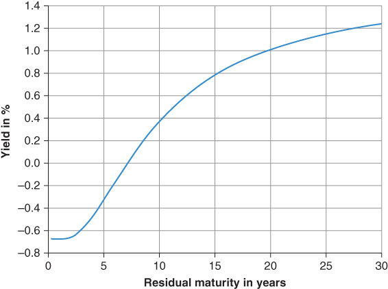
Graphical illustration of the Eurozone AAA sovereign bond yield curve for 15 June 2017. — *Figure 6.3* Eurozone AAA sovereign bond yield curve, 15 June 2017
*Source*: https://www.ecb.europa.eu/stats/financial_markets_and_interest_rates/euro_area_yield_curves/html/index.en.html

A continuous negative rates environment places difficulties on the ALM desk in a bank. In general, the approach to operating in these conditions may involve the following:

Ideally, pass on the negative interest rate to deposit customers. This is not usually possible for relationship and reputation reasons, or for retail and small business customers, but is common for larger corporate customers;
Within the constraints placed by sound liquidity risk management policy (see Chapter 9), avoid running too large surplus deposit balances and seek to lend surplus liabilities as much as possible within individual bank loan policy constraints;
Seek to raise stable long‐dated customer funding while deposit rates are low, paying a lower premium than would otherwise be the case in a conventional positive curve environment;
Consider strategies involving exchanging the surplus domestic currency deposits into another currency so that there is no need to place them with the home central bank, and investing in assets denominated in the foreign currency. This, of course, creates associated FX market risk, which must be monitored and mitigated, and an appropriate risk appetite statement regarding this must be approved.

From the ALM desk perspective, the negative rates charged by the central bank will need to be considered for incorporation in the bank's funds transfer pricing policy (FTP – see Chapter 11), although as noted above in the retail customer space, where loans will still be made at a positive rate of interest, deposits will not necessarily be charged at a negative rate.

In general, while euro‐area and Japanese banks will have learnt to operate in a negative rates environment, and despite the fact that the ECB has operated its negative base rate policy for some years, negative interest rates remain “non‐normal” and are a sign of economic stagnation.

CREDIT INTERMEDIATION BY THE REPO DESK

In general, for banks with access to repo and bond stock loan markets, the government bond repo market will trade at a lower rate than other money market instruments, reflecting its status as a secured instrument with the best credit. This allows spreads between markets of different credits to be exploited. The following are examples of credit intermediation trades:

A repo dealer lends general collateral (GC) currently trading at a spread below Libor and uses the cash to buy certificates of deposit (CDs) trading at a spread above Libor;
A repo dealer borrows specific collateral in the stock‐lending market – paying a fee – and sells the stock in the repo market at the GC rate; the cash is then lent in the inter‐bank market at a higher rate – for instance, through the purchase of a clearing bank certificate of deposit. The CD is used as collateral in the stock loan transaction. A bank must have dealing relationships with both the stock loan and repo markets to effect this trade. An example of the trade that could be put on using this type of intermediation is shown in Figure 4.3 for the UK gilt market. The details are given below and show that the bank would stand to gain 17 basis points over the course of the 3‐month trade;
A repo dealer trades repo in the GC market, and using the cash from this repo invests in emerging market collateral at a spread, say, 400 basis points higher.

These are but three examples of the way that repo can be used to exploit the interest‐rate differentials that exist between markets of varying credit qualities and between secured and unsecured markets.

Figure 6.4 shows potential gains that can be made by a repo‐dealing bank (market‐maker) that has access to both the stock loan and general collateral repo market. It illustrates the rates available in the gilt market on 31 October 2000 for 3‐month maturities, which were:

3‐month GC repo	5.83–5.75%
3‐month clearing bank CD	6132–6.00%

Schematic illustration of an intermediation between stock loan and repo markets; an example using UK gilts. — *Figure 6.4* Intermediation between stock loan and repo markets; an example using UK gilts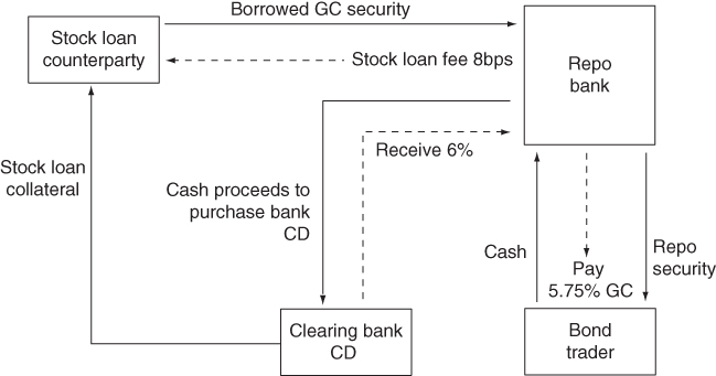

The stock loan fee for this term was quoted at 510 basis points, with the actual fee paid being 8 basis points. Therefore, the repo trader borrows GC stock for 3 months and offers this in repo at 5.75%.³ The cash proceeds are then used to purchase a clearing bank CD at 6.00%. This CD is used as collateral in the stock loan. The profit is market risk free as the terms are locked, although there is an element of credit risk in holding the CD. On these terms, the profit in £100 million stock for the 3‐month period is approximately £170,000.

The main consideration for the dealing bank is the capital requirements of the trade. Gilt repo is zero weighted for capital purposes. Indeed, clearing bank CDs are accepted by the Bank of England for liquidity purposes, so the capital cost is not onerous. The bank will need to ensure that it has sufficient credit lines for the repo and CD counterparties.

Example 6.1 ALM considerations

Assume that a bank may access the markets for 3‐month and 6‐month funds, whether for funding or investment purposes. The rates for these terms are shown in Table 6.1. Assume no bid–offer spreads. The ALM manager also expects the 3‐month Libor rate in 3 months' time to be 5.10%. The bank can usually fund its book at Libor, while it is able to lend at Libor plus 1%.

Table 6.1 Hypothetical money market rates

Term	Libor	Bank rate
90‐day	5.50%	6.50%
180‐day	5.75%	6.75%

Expected 90‐day rate	5.10%	6.10%
in 90 days' time
3v6 forward rate agreement (FRA)	6.60%

The bank could adopt any of the following strategies, or a combination of them:

Borrow 3‐month funds at 5.50% and lend this out in the 3‐month at 6.50%. This locks‐in a return of 1% for a 3‐month period;
Borrow 6‐month funds at 5.75% and lend in the 6‐month at 6.75%; again this earns a locked‐in spread of 1%;
Borrow 3‐month funds at 5.50% and lend this in the 6‐month at 6.75%. This approach would require the bank to refund the loan in 3 months' time, which it expects to be able to do at 5.10%. This approach locks‐in a return of 1.25% in the first 3‐month period, and an expected return of 1.65% in the second 3‐month period. The risk of this tactic is that the 3‐month rate in 3 months' time does not fall as expected by the ALM manager, reducing profits and possibly leading to loss;
Borrow in the 6‐month at 5.75% and lend these for a 6‐month period at 6.50%. After this period, lend the funds in the 3‐month or 6‐month. This strategy does not tally with the ALM manager's view, however, who expects a fall in rates and so should not wish to be long of funds in 3 months' time;
Borrow 3‐month funds at 5.50% and again lend this in the 3‐month at 6.75%. To hedge the gap risk, the ALM manager simultaneously buys a 3v6 FRA to lock‐in the 3‐month rate in 3 months' time. The first period spread of 1.25% is guaranteed, but the FRA guarantees only a spread of 15 basis points in the second period. This is the cost of the hedge (and also suggests that the market does not agree with the ALM manager's assessment of where rates will be 3 months from now!), the price the bank must pay for reducing uncertainty, the lower spread return. Alternatively, the bank could lend in the 6‐month period, funding initially in the 6‐month, and buy an interest‐rate cap with a ceiling rate of 6.60% and pegged to Libor, the rate at which the bank can actually fund its book.

Although somewhat stylistic, these scenarios serve to illustrate what is possible, and indeed there are many other strategies that could be adopted. The approaches described in the last option show how derivative instruments can be used actively to manage the banking book, and the cost that is associated with employing them.

Example 6.2 Position management

Starting the day with a flat position, a money market interbank desk transacts the following deals:

£100 million borrowing from 16/9/09 to 7/10/09 (3 weeks) at 6.375%
£60 million borrowing from 16/9/09 to 16/10/09 (1 month) at 6.25%
£110 million loan from 16/9/09 to 18/10/09 (32 days) at 6.45%.

The desk reviews its cash position and the implications for refunding and interest‐rate risk, bearing in mind the following:

There is an internal overnight roll‐over limit of £40 million (net);
The bank's economist feels more pessimistic about a rise in interest rates than most others in the market, and has recently given an internal seminar on the dangers of inflation in the UK as a result of recent increases in the level of average earnings;
Today there are some important figures being released including inflation (RPI) data. If today's RPI figures exceed market expectations, the dealer expects a tightening of monetary policy by at least 0.50% almost immediately;
A broker's estimate of daily market liquidity for the next few weeks is one of low shortage, with little central bank intervention required, and hence low volatilities and rates in the overnight rate;
Brokers' screens indicate the following term repo rates:

O/N 6.350–6.300%

1 week 6.390–6.340%

2 week 6.400–6.350%

1 month 6.410–6.375%

2 month 6.500–6.450%

3 month 6.670–6.620%
The indication for a 1v2 FRA is:

1v2 FRA 6.680–6.630%
The quote for an 11‐day forward borrowing in 3 weeks' time (the “21v32 rate”) is 6.50% bid.

The book's exposure looks like the illustration in Figure 6.5.

Figure 6.5 Position timeline

What courses of action are open to the desk, bearing in mind that the book needs to be squared off such that the position is flat each night?

Possible solutions

Investing early surplus

From a cash management point of view, the desk has a £50 million surplus from 16/9 up to 7/10. This needs to be invested. It may be able to negotiate a 6.31% loan with the market for overnight, or 6.35% term deposit for 1 week to 6.38% for 1 month.

The overnight roll is the most flexible but offers a worse rate, and if the desk expects the overnight rate to remain both low and stable (due to forecasts of low market shortages), it may not opt for this course of action.

However, it may make sense from an interest‐rate risk point of view. If the desk agrees with the bank's economist, it should be able to benefit from rolling at higher rates soon – possibly in the next 3 weeks. Therefore, it may not want to lock in a term rate now, and the overnight roll would match this view. However, it exposes them to lower rates, if their view is wrong, which will limit the extent of the positive funding spread. The market itself appears neutral about rate changes in the next month, but appears to factor in a rise thereafter.

The forward “gap”

Looking forward, the book is currently on course to exceed the £40 million overnight position limit on 7/10, when the refunding requirement is £50 million. The situation gets worse on 16/10 (for 2 days) when the refunding requirement is £110 million. The desk needs to fix a term deal before those dates to carry it over until 18/10 when the funding position reverts to zero. A borrowing from 7/10 to 18/10 of £50 million will reduce the rollover requirement to within limit.

However, given that interest rates will rise, should the desk wait until the 7th to deal in the cash? Not if it has a firm view. They may end up paying as much as 6.91% or higher for the funding (after the 0.50% rate rise). So it would be better to transact now a forward starting repo to cover the period, thus locking in the benefits obtainable from today's yield curve. The market rate for a 21 × 32‐day repo is quoted at 6.50%. This reflects the market's consensus that rates may rise in about a month's time. However, the desk's own expectation is of a larger rise, hence its own logic suggests trading in the forward loan. This strategy will pay dividends if their view is right, as it limits the extent of funding loss.

An alternative means of protecting the interest‐rate risk alone is to BUY a 1v2 month Forward Rate Agreement (FRA) for 6.68%. This does not exactly match the gap, but should act as an effective hedge. If there is a rate rise, the book gains from the FRA profit. Note that the cash position still needs to be squared off. Should the desk deal before or after the inflation announcement? That is, of course, down to its judgement, but most dealers like, if at all possible, to sit tight ahead of releases of key economic data.

INTEREST‐RATE HEDGING TOOLS

For bank dealers who are not looking to trade around term mismatch or other spreads, but who will run a tenor mismatch between assets and liabilities (which is, after all, what banking is: the practice of maturity transformation), there are a number of instruments they can use to hedge the resulting interest‐rate risk exposure. We consider them briefly here.

Interest‐rate futures

A forward term interest‐rate gap exposure can be hedged using interest‐rate futures. These are standardised exchange‐traded derivative contracts, and represent a forward‐starting 90‐day time deposit. In the sterling market, the instrument will typically be the 90‐day short sterling future traded on London's “LIFFE” futures exchange. A strip of futures can be used to hedge the term gap. The trader buys futures contracts to the value of the exposure and for the term of the gap. Any change in cash rates should be hedged by offsetting moves in futures prices.

Description

A futures contract is a transaction that fixes the price today for a commodity that will be delivered at some point in the future. Financial futures fix the price for interest rates, bonds, equities, and so on, but trade in the same manner as commodity futures. Contracts for futures are standardised and traded on recognised exchanges. In London, the main futures exchange is LIFFE, although other futures are also traded on, for example, the International Petroleum Exchange and the London Metal Exchange. Money markets trade short‐term interest‐rate futures that fix the rate of interest on a notional fixed term deposit of money (usually for 90 days or 3 months) for a specified period in the future. The sum is notional because no actual sum of money is deposited when buying or selling futures – the instrument being off‐balance‐sheet. Buying such a contract is equivalent to making a notional deposit, while selling a contract is equivalent to borrowing a notional sum.

The 3‐month interest‐rate future is the most widely used instrument for hedging interest‐rate risk.

The LIFFE exchange in London trades short‐term interest‐rate futures for major currencies including sterling, euros, yen, and the Swiss franc. Table 6.2 summarises the terms for the short sterling contract as traded on LIFFE.

Table 6.2 Description of LIFFE short sterling futures contract

Source: LIFFE.

Name	90‐day sterling Libor interest‐rate future
Contract size	£500,000
Delivery months	March, June, September, December
Delivery date	First business day after the last trading day
Last trading day	Third Wednesday of delivery month
Price	100 minus interest rate
Tick size	0.01
Tick value	£12.50
Trading hours	LIFFE CONNECT™ 07:30–18:00 hours

Futures contracts originally related to physical commodities, which is why we speak of delivery when referring to the expiry of financial futures contracts. Exchange‐traded futures such as those on LIFFE are set to expire every quarter during the year. The short sterling contract is a deposit of cash, so as its price refers to the rate of interest on this deposit, the price of the contract is set as P = 100r where P is the price of the contract and r is the rate of interest at the time of expiry implied by the futures contract. This means that if the price of the contract rises, the rate of interest implied goes down and vice versa. For example, the price of the June 2011 short sterling future (written as Jun11 or M11, from the futures identity letters of H, M, U, and Z for contracts expiring in March, June, September, and December, respectively) at the start of trading on 22 September 2010 was 99.05, which implied a 3‐month Libor rate of 0.95% on expiry of the contract in June 2011. If a trader bought 20 contracts at this price and then sold them just before the close of trading that day, when the price had risen to 99.08, an implied rate of 0.92%, she would have made 3 ticks profit or £750. That is, a 3‐tick upward price movement in a long position of 20 contracts is equal to £750. This is calculated as follows:

$images$

The tick value for the short sterling contract is straightforward to calculate. Since we know that the contract size is £500,000, there is a minimum price movement (tick movement) of 0.01% and the contract has a 3‐month “maturity”:

$images$

The profit made by the trader in our example is logical because if we buy short sterling futures we are depositing (notional) funds and if the price of the futures rises, it means the interest rate has fallen. We profit because we have “deposited” funds at a higher rate beforehand. If we expected sterling interest rates to rise, we would sell short sterling futures, which is equivalent to borrowing funds and locking in the loan rate at a lower level.

Note how the concept of buying and selling interest‐rate futures differs from FRAs: if we buy an FRA we are borrowing notional funds, whereas if we buy a futures contract we are depositing notional funds. If a position in an interest‐rate futures contract is held to expiry, cash settlement will take place on the delivery day for that contract.

Short‐term interest‐rate contracts in other currencies are similar to the short sterling contract and trade on exchanges such as Deutsche Terminbörse in Frankfurt and MATIF in Paris.

In practice, futures contracts do not provide a precise tool for locking into cash market rates today for a transaction that takes place in the future, although this is what they are theoretically designed to do. Futures do allow a bank to lock in a rate for a transaction to take place in the future; this rate is the forward rate. The basis is the difference between today's cash market rate and the forward rate on a particular date in the future. As a futures contract approaches expiry, its price and the rate in the cash market will converge (the process is given the name convergence). This is given by the exchange delivery settlement price, and the two prices (rates) will be exactly in line at the precise moment of expiry.

Example 6.3 The Eurodollar futures contract

The Eurodollar futures contract is traded on the Chicago Mercantile Exchange. The underlying asset is a deposit of US dollars in a bank outside the US, and the contract is at the rate of dollar 90‐day Libor. The Eurodollar future is cash settled on the second business day before the third Wednesday of the delivery month (London business day). The final settlement price is used to set the price of the contract, given by:

$images$

where r is the quoted Eurodollar rate at the time. This rate is the actual 90‐day Eurodollar deposit rate.

The longest dated Eurodollar contract has an expiry date of 10 years. The market assumes that futures prices and forward prices are equal; this is indeed the case under conditions where the risk‐free interest rate is constant and the same for all maturities. In practice, it also holds for short‐dated futures contracts, but does not for longer dated futures contracts. Therefore, using futures contracts with a maturity greater than 5 years to calculate zero‐coupon rates or implied forward rates will produce errors in results, which need to be taken into account if the derived rates are used to price other instruments such as swaps.

Hedging using interest‐rate futures

Banks use interest‐rate futures to hedge interest‐rate risk exposure in cash and OBS instruments. Bond‐trading desks often use futures to hedge positions in bonds of up to 2 or 3 years' maturity, as contracts are traded up to 3 years' maturity. The liquidity of such “far month” contracts is considerably lower than for “near month” contracts and the “front month” contract (the current contract for the next maturity month). When hedging a bond with a maturity of, say, 2 years' maturity, the trader will put on a strip of futures contracts that matches as near as possible the expiry date of the bond.

The purpose of a hedge is to protect the value of a current or anticipated cash market or OBS position from adverse changes in interest rates. The hedger will try to offset the effect of the change in interest rate on the value of his cash position with the change in value of his hedging instrument. If the hedge is an exact one the loss on the main position should be compensated by a profit on the hedge position. If the trader is expecting a fall in interest rates and wishes to protect against such a fall, he will buy futures (known as a long hedge) and will sell futures (a short hedge) if wishing to protect against a rise in rates.

Bond traders also use 3‐month interest‐rate contracts to hedge positions in short‐dated bonds; for instance, a market‐maker running a short‐dated bond book would find it more appropriate to hedge his book using short‐dated futures rather than the longer dated bond futures contract. When this happens it is important to accurately calculate the correct number of contracts to use for the hedge. To construct a bond hedge it will be necessary to use a strip of contracts, thus ensuring that the maturity date of the bond is covered by the longest dated futures contract. The hedge is calculated by finding the sensitivity of each cash flow to changes in each of the relevant forward rates. Each cash flow is considered individually and hedge values are then aggregated and rounded to the nearest whole number of contracts.

Examples 6.4 and 6.5 illustrate hedging with short‐term interest‐rate contracts.

Example 6.4 Hedging a forward 3‐month lending requirement

On 1 June a corporate treasurer is expecting a cash inflow of £10 million in 3 months' time (1 September), which he will then invest for 3 months. The treasurer expects interest rates will fall over the next few weeks and wishes to protect himself against such a fall. This can be done using short sterling futures. The market rates on 1 June are as follows:

3‐month Libor	$images$
Sep futures price	93.220

The treasurer buys 20 September short sterling futures at 93.220, this number being exactly equivalent to a sum of £10 million. This allows him to lock in a forward lending rate of 6.78%, on the assumption there is no bid–offer quote spread:

$images$

On 1 September the market rates are as follows:

3‐month Libor	612%
Sep futures price	93.705

The treasurer unwinds the hedge at this price.

$images$

The treasurer was quite close to achieving his target lending rate of 6.78% and the hedge has helped to protect against the drop in Libor rates from $images$ to $images$ , as a result of the profit from the futures transaction.

In the real world, the cash market bid–offer spread will impact the amount of profit/loss from the hedge transaction. Futures generally trade and settle near the offered side of the market rate (Libor), whereas lending, certainly by corporates, will be nearer the Libid rate.

Example 6.5 Hedging a forward 6‐month borrowing requirement

A Treasury dealer has a 6‐month borrowing requirement for EUR30 million in 3 months' time, on 16 September. He expects interest rates to rise by at least 12% before that date and would like to lock in a future borrowing rate. The scenario is:

Date	16 June
3‐month Libor	6.0625%
6‐month Libor	6.25
Sep futures contract	93.66
Dec futures contract	93.39

In order to hedge a 6‐month EUR30 million exposure, the dealer needs to use a total of 60 futures contracts, as each has a nominal value of EUR1 million, and corresponds to a 3‐month notional deposit period. The dealer decides to sell 30 September futures contracts and 30 December futures contracts. This is referred to as a strip hedge. The expected forward borrowing rate that can be achieved by this strategy, where the expected borrowing rate is rf, is calculated as follows:

$images$

Therefore, we have:

$images$

The rate rf is sometimes referred to as the “strip rate”.

The hedge is unwound upon expiry of the September futures contract. Assume the following rates now prevail:

3‐month Libor	6.4375%
6‐month Libor	6.8125%
Sep futures contract	93.56
Dec futures contract	92.93

The futures P&L is:

September contract	+10 ticks
December contract	+46 ticks

This represents a 56‐tick or 0.56% profit in 3‐month interest‐rate terms, or 0.28% in 6‐month interest‐rate terms. The effective borrowing rate is the 6‐ month Libor rate minus the futures profit, or:

$images$

In this case the hedge has proved effective because the dealer has realised a borrowing rate of 6.5325%, which is close to the target strip rate of 6.53%.

The dealer is still exposed to the basis risk when the December contracts are bought back from the market at the expiry date of the September contract. If, for example, the future was bought back at 92.73, the effective borrowing rate would only be 6.4325%, and the dealer would benefit. Of course, the other possibility is that the futures contract could be trading 20 ticks more expensive, which would give a borrowing rate of 6.6325%, which is 10 basis points above the target rate. If this happened, the dealer may elect to borrow in the cash market for 3 months, maintain the December futures position until the December contract expiry date, and roll over the borrowing at that time. The profit (or loss) on the December futures position will compensate for any change in 3‐month rates at that time.

Forward rate agreements

Forward rate agreements (FRAs) are similar in concept to interest‐rate futures and like them are off‐balance‐sheet instruments. Under an FRA a buyer agrees notionally to borrow and a seller to lend a specified notional amount at a fixed rate for a specified period – the contract to commence on an agreed date in the future. On this date (the “fixing date”), the actual rate is taken and, according to its position versus the original trade rate, the borrower or lender will receive an interest payment on the notional sum equal to the difference between the trade rate and the actual rate. The sum paid over is present valued as it is transferred at the start of the notional loan period, whereas in a cash market trade interest would be handed over at the end of the loan period. As FRAs are off‐balance‐sheet contracts no actual borrowing or lending of cash takes place, hence the use of the term “notional”. In hedging an interest‐rate gap in the cash period, the trader will buy an FRA contract that equates to the term gap for a nominal amount equal to his exposure in the cash market. Should rates move against him in the cash market, the gain on the FRA should (in theory) compensate for the loss in the cash trade.

Definition of an FRA

An FRA is an agreement to borrow or lend a notional cash sum for a period of time lasting up to 12 months, starting at any point over the next 12 months, at an agreed rate of interest (the FRA rate). The “buyer” of an FRA is borrowing a notional sum of money, while the “seller” is lending this cash sum. Note how this differs from all other money market instruments. In the cash market, the party buying a CD or bill, or bidding for stock in the repo market, is the lender of funds. In the FRA market, to “buy” is to “borrow”. Of course, we use the term “notional” because with an FRA no borrowing or lending of cash actually takes place. The notional sum is simply the amount on which interest payment is calculated.

So, when an FRA is traded, the buyer is borrowing (and the seller is lending) a specified notional sum at a fixed rate of interest for a specified period – the “loan” to commence at an agreed date in the future. The buyer is the notional borrower, and so she will be protected if there is a rise in interest rates between the date that the FRA is traded and the date that the FRA comes into effect. If there is a fall in interest rates, the buyer must pay the difference between the rate at which the FRA was traded and the actual rate, as a percentage of the notional sum. The buyer may be using the FRA to hedge an actual exposure – that is, an actual borrowing of money – or simply speculating on a rise in interest rates. The counterparty to the transaction, the seller of the FRA, is the notional lender of funds, and has fixed the rate for lending funds. If there is a fall in interest rates the seller will gain, and if there is a rise in rates the seller will pay. Again, the seller may have an actual loan of cash to hedge or be a speculator.

In FRA trading only the payment that arises as a result of the difference in interest rates changes hands. There is no exchange of cash at the time of the trade. The cash payment that does arise is the difference in interest rates between that at which the FRA was traded and the actual rate prevailing when the FRA matures, as a percentage of the notional amount. FRAs are traded by both banks and corporates and between banks. The FRA market is very liquid in all major currencies and rates are readily quoted on screens by both banks and brokers. Dealing is over the telephone or over a dealing system such as Reuters.

The terminology quoting FRAs refers to the borrowing time period and the time at which the FRA comes into effect (or matures). Hence, if a buyer of an FRA wished to hedge against a rise in rates to cover a 3‐month loan starting in 3 months' time, she would transact a “3‐against‐6‐month” FRA, more usually denoted as a 3–6s or 3v6 FRA. This is referred to in the market as a “threes–sixes” FRA, and means a 3‐month loan beginning in 3 months' time. So, correspondingly, a “ones–fours” FRA (1v4) is a 3‐month loan in 1 month's time, and a “threes–nines” FRA (3v9) is a 6‐month loan in 3 months' time.

Remember that when we buy an FRA we are “borrowing” funds. This differs from cash products such as a CD or repo, as well as interest‐rate futures, where to “buy” is to lend funds.

Example 6.6 FRA hedging

A company knows that it will need to borrow £1 million in 3 months' time for a 12‐month period. It can borrow funds today at Libor 50 basis points. Libor rates today are at 5% but the company's treasurer expects rates to go up to about 6% over the next few weeks. So, the company will be forced to borrow at higher rates unless some sort of hedge is transacted to protect the borrowing requirement. The treasurer decides to buy a 3v15 (“threes–fifteens”) FRA to cover the 12‐month period beginning 3 months from now. A bank quotes $images$ for the FRA, which the company buys for a notional £1 million. After 3 months the rates have indeed gone up to 6%, so the treasurer must borrow funds at $images$ (the Libor rate plus spread). However, she will receive a settlement amount that will be the difference between the rate at which the FRA was bought and today's 12‐month Libor rate (6%) as a percentage of £1 million, which will compensate for some of the increased borrowing costs.

FRA mechanics

In virtually every market, FRAs trade under a set of terms and conventions that are identical. The British Bankers Association (BBA) has compiled standard legal documentation to cover FRA trading. The following standard terms are used in the market:

Notional sum: the amount for which the FRA is traded;
Trade date: the date on which the FRA is dealt;
Settlement date: the date on which the notional loan or deposit of funds becomes effective; that is, is said to begin. This date is used, in conjunction with the notional sum, for calculation purposes only as no actual loan or deposit takes place;
Fixing date: this is the date on which the reference rate is determined; that is, the rate with which the FRA dealing rate is compared;
Maturity date: the date on which the notional loan or deposit expires;
Contract period: the time between the settlement date and maturity date;
FRA rate: the interest rate at which the FRA is traded;
Reference rate: the rate used as part of the calculation of the settlement amount, usually the Libor rate on the fixing date for the contract period in question;
Settlement sum: the amount calculated as the difference between the FRA rate and the reference rate as a percentage of the notional sum, paid by one party to the other on the settlement date.

These dates are illustrated in Figure 6.6.

Schematic illustration of key dates in a forward rate agreement (FRA) trade. — *Figure 6.6* Key dates in an FRA trade

The spot date is usually 2 business days after the trade date; however, it can by agreement be sooner or later than this. The settlement date will be the time period after the spot date referred to by FRA terms – for example, a $images$ FRA will have a settlement date 1 calendar month after the spot date. The fixing date is usually 2 business days before the settlement date. The settlement sum is paid on the settlement date and, as it refers to an amount over a period of time that is paid upfront at the start of the contract period, the calculated sum is a discounted present value. This is because a normal payment of interest on a loan/deposit is paid at the end of the time period to which it relates. Because an FRA makes this payment at the start of the relevant period, the settlement amount is also a discounted present value sum.

With most FRA trades the reference rate is the Libor setting on the fixing date.

The settlement sum is calculated after the fixing date, for payment on the settlement date. We may illustrate this with a hypothetical example. Consider the case where a corporate has bought £1 million notional of a 1v4 FRA and dealt at 5.75%, and that the market rate is 6.50% on the fixing date. The contract period is 90 days. In the cash market, the extra interest charge that the corporate would pay is a simple interest calculation:

$images$

The extra interest that the corporate is facing would be payable with the interest payment for the loan, which (as it is a money market loan) is when the loan matures. Under an FRA, then, the settlement sum payable should be exactly equal to this if it was paid on the same day as the cash market interest charge. This would make it a perfect hedge. However, as we noted above, the FRA settlement value is paid at the start of the contract period – that is, at the beginning of the underlying loan and not the end. Therefore, the settlement sum has to be adjusted to account for this, and the amount of the adjustment is the value of the interest that would be earned if the unadjusted cash value was invested for the contract period in the money market. The settlement value is given by equation (6.1):

(6.1) $images$

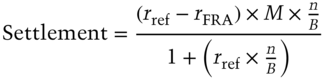
where

r_ref	=	Reference interest fixing rate;
r_FRA	=	FRA rate or contract rate;
M	=	Notional value;
n	=	Number of days in the contract period;
B	=	Day‐count base (360 or 365).

Equation 6.1 simply calculates the extra interest payable in the cash market, resulting from the difference between the two interest rates, and then discounts the amount because it is payable at the start of the period and not, as would happen in the cash market, at the end of the period.

In our hypothetical illustration, the corporate buyer of the FRA receives the settlement sum from the seller as the fixing rate is higher than the dealt rate. This then compensates the corporate for the higher borrowing costs that he would have to pay in the cash market. If the fixing rate had been lower than 5.75%, the buyer would pay the difference to the seller, because cash market rates will mean that he is subject to a lower interest rate in the cash market. What the FRA has done is hedge the interest rate, so that whatever happens in the market, it will pay 5.75% on its borrowing.

A market‐maker in FRAs is trading short‐term interest rates. The settlement sum is the value of the FRA. The concept is exactly the same as with trading short‐term interest‐rate futures; a trader who buys an FRA is running a long position, so that if r_ref > r_FRA on the fixing date the settlement sum is positive and the trader realises a profit. What has happened is that the trader, by buying the FRA, “borrowed” money at an interest rate that subsequently rose. This is a gain, exactly like a short position in an interest‐rate future, where if the price goes down – that is, interest rates go up – the trader realises a gain. Equally, a “short” position in an FRA, put on by selling an FRA, realises a gain if r_ref < r_FRA on the fixing date.

FRA pricing

As their name makes clear, FRAs are forward rate instruments and are priced using standard forward rate principles.⁴ Consider an investor who has two alternatives: either a 6‐month investment at 5% or a 1‐year investment at 6%. If the investor wishes to invest for 6 months and then roll over the investment for a further 6 months, what rate is required for the rollover period such that the final return equals the 6% available from the 1‐year investment? If we view an FRA rate as the breakeven forward rate between the two periods, we simply solve for this forward rate. The result is our approximate FRA rate.

We can use the standard forward rate breakeven formula to solve for the required FRA rate. The relationship given in equation (6.2) connects simple (bullet) interest rates for periods of time up to 1 year, where no compounding of interest is required. As FRAs are money market instruments we are not required to calculate rates for periods in excess of 1 year,⁵ where compounding would need to be built into the equation. The expression is:

(6.2) $images$

where

r₂	=	Cash market interest rate for the long period;
r₁	=	Cash market interest rate for the short period;
r_f	=	Forward rate for the gap period;
t₂	=	Time period from today to the end of the long period;
t₁	=	Time period from today to the end of the short period;
t_f	=	Forward gap time period, or the contract period for the FRA.

This is illustrated diagrammatically in Figure 6.7.

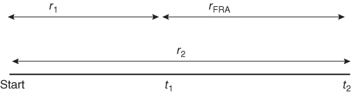
Schematic illustration of the rates used in forward rate agreement (FRA) pricing. — *Figure 6.7* Rates used in FRA pricing

The time period t₁ is the time from the dealing date to the FRA settlement date, while t₂ is the time from the dealing date to the FRA maturity date. The time period for the FRA (contract period) is t₂ minus t₁. We can replace the symbol “t” for time period with “n” for the actual number of days in the time periods themselves. If we do this and then rearrange the equation to solve for r_FRA (the FRA rate) we obtain:

(6.3) $images$

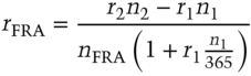
where

n₁	=	Number of days from the dealing date or spot date to the settlement date;
n₂	=	Number of days from the dealing date or spot date to the maturity date;
r₁	=	Spot rate to the settlement date;
r₂	=	Spot rate from the spot date to the maturity date;
n_FRA	=	Number of days in the FRA contract period;
r_FRA	=	FRA rate.

If the formula is applied to, say, US dollar money markets, the 365 in the equation is replaced by 360, the day‐count base for that market.

In practice, FRAs are priced off the exchange‐traded short‐term interest‐rate future for that currency, so that sterling FRAs are priced off LIFFE short sterling futures. Traders normally use a spreadsheet pricing model that has futures prices directly fed into it. FRA positions are also usually hedged with other FRAs or short‐term interest‐rate futures.

Example 6.7 Hedging an FRA position

An FRA market‐maker sells a EUR100 million 3 × 6 FRA, i.e. an agreement to make a notional deposit (without exchange of principal) for 3 months in 3 months' time at a rate of 7.52%. He is exposed to the risk that interest rates will have risen by the FRA settlement date in 3 months' time.

Action

The dealer first needs to calculate a precise hedge ratio. This is a three‐stage process:

Calculate the nominal value of a basis point move in Libor on the FRA settlement payment:
$images$
Therefore:
$images$
Find the present value of (i) by discounting it back to the transaction date using the FRA and spot rates:
$images$
Therefore:
$images$
Determine the correct hedge ratio by dividing (ii) by the futures tick value.
$images$

The appropriate number of contracts for the hedge of a EUR100,000,000 3 × 6 FRA would therefore be 96 or 97, as the fraction is under one‐half, 96 is correct.

To hedge the risk of an increase in interest rates, the trader sells 96 EUR 3 months futures contracts at 92.50. Any increase in rates during the hedge period should be offset by a gain realised on the futures contracts through daily variation margin receipts.

Outcome

Date	15 March
3‐month Libor	7.625%
March EDSP	92.38

The hedge is lifted upon expiry of the March futures contracts. The 3‐month Libor on the FRA settlement date has risen to 7.625%, so the trader incurs a loss of EUR25,759 on his FRA position (i.e. EUR26,250 discounted back over the 3‐month FRA period at current Libor rate), calculated as follows:

$images$

Therefore:

$images$

Futures P/L:

$images$

Conclusion

The EUR25,759 loss on the FRA position is more than offset by the EUR28,800 profit on the futures position when the hedge is lifted.

If the dealer has sold 100 contracts, his futures profit would have been EUR30,000, and, accordingly, been a less accurate hedge. The excess profit in the hedge position can mostly be attributed to the arbitrage profit realised by the market‐maker (i.e. the market‐maker has sold the FRA for 7.52% and in effect bought it back in the futures market by selling futures at 92.50 or 7.50% for a 2 tick profit).

Interest‐rate swaps

An interest‐rate swap is an off‐balance‐sheet agreement between two parties to make periodic interest payments to each other. Payments are on a predetermined set of dates in the future, based on a notional principal amount; one party is the fixed‐rate payer, the rate agreed at the start of the swap, and the other party is the floating‐rate payer, the floating‐rate being determined during the life of the swap by reference to a specific market rate or index. There is no exchange of principal, only of the interest payments on this principal amount. Note that our description is for a plain vanilla swap contract; it is common to have variations on this theme – for instance, floating–floating swaps where both payments are floating‐rate, as well as cross‐currency swaps where there is an exchange of an equal amount of different currencies at the start dates and end dates of the swap.

An interest‐rate swap can be used to hedge the fixed‐rate risk arising from originating a loan at a fixed interest rate, such as a fixed‐rate mortgage. The terms of the swap should match the payment dates and maturity date of the loan. The idea is to match the cash flows from the loan with equal and opposite payments in the swap contract, which will hedge the mortgage position. For example, if the retail bank has advanced a fixed‐rate mortgage, it will be receiving fixed‐rate coupon payments on the nominal value of the loan (together with a portion of the capital repayment if it is a repayment mortgage and not an interest‐only mortgage). To hedge this position, the trader buys a swap contract for the same nominal value in which he will be paying the same fixed‐rate payment; net cash flow is a receipt of floating interest‐rate payments.

A borrower, on the other hand, may issue bonds of a particular type because of investor demand for such paper, but prefer to have the interest exposure on the debt in some other form. So, for example, a UK company issues fixed‐rate bonds denominated in, say, Australian dollars, swaps the proceeds into sterling, and pays floating‐rate interest on the sterling amount. As part of the swap the company will be receiving fixed‐rate Australian dollars, which neutralises the exposure arising from the bond issue. On termination of the swap (which must coincide with the maturity of the bond), the original currency amounts are exchanged back, enabling the issuer to redeem the holders of the bond in Australian dollars.

For detailed coverage of interest‐rate swaps and their application, see Choudhry (2014), which includes a discussion on post‐crash swap pricing principles.

Description

Swaps are derivative contracts involving combinations of two or more interest‐rate bases or other building blocks. Most swaps currently traded in the market involve combinations of cash market securities – for example, a fixed interest‐rate security combined with a floating interest‐rate security, possibly also combined with a currency transaction. However, the market has also seen swaps that involve a futures or forward component, as well as swaps that involve an option component. The market for swaps is organised by the International Swaps and Derivatives Association (ISDA).

Example 6.8 Comparative advantage and interest‐rate swap structure

When entering into a swap either for hedging purposes or to alter the basis of an interest‐rate liability, the opposite of a current cash flow profile is required. Consider a homeowner with a variable rate mortgage. The homeowner is at risk from an upward move in interest rates, which will result in her being charged higher interest payments. She wishes to protect herself against such a move and in theory (don't try this with your building society!), as she is paying floating, she must receive floating in a swap. Therefore, she will pay fixed in the swap. The floating interest payments cancel each other out, and the homeowner now has a fixed‐rate liability. The same applies in a hedging transaction: a bondholder receiving fixed coupons from the bond issuer – that is, the bondholder is a lender of funds – can hedge against a rise in interest rates that lowers the price of the bond by paying fixed in a swap with the same basis point value as the bond position; the bondholder receives floating interest. Paying fixed in a swap is conceptually the same as being a borrower of funds; this borrowing is the opposite of a loan of funds to the bond issuer and therefore the position is hedged. Consider two companies' borrowing costs for a 5‐year loan of £50 million:

Company A can pay fixed at 8.75% or floating at Libor. Its desired basis is floating;
Company B can pay fixed at 10% or floating at Libor + 100 basis points. Its desired basis is fixed.

Without a swap:

Company A borrows fixed and pays 8.75%.
Company B borrows floating and pays Libor + 100 basis points.

Let us say that the two companies decide to enter into a swap, whereby Company A borrows floating‐rate interest and therefore receives fixed from Company B at the 5‐year swap rate of 8.90%. Company B, which has borrowed at Libor + 100 basis points, pays fixed and receives Libor in the swap. Company A ends up paying floating‐rate interest and Company B ends up paying fixed.

The result after the swap:

$images$

Company A saves 15 basis points (pays L–15bp rather than L flat) and B saves 10 basis points (pays 9.90% rather than 10%).

Both parties benefit from the comparative advantage of A in the fixed‐rate market and B in the floating‐rate market (spread of B over A is 125bp in the fixed‐rate market but 100bp in the floating‐rate market). Originally, swap banks were simply brokers, and charged a fee to both counterparties for bringing them together. In the example, Company A deals directly with Company B, although it is more likely that an intermediary bank would have been involved. As the market developed, banks became principals and dealt directly with counterparties, eliminating the need to find someone who had requirements that could be met by the other side of an existing requirement.

An interest‐rate swap is an agreement between two counterparties to make periodic interest payments to one another during the life of the swap, on a predetermined set of dates, based on a notional principal amount. One party is the fixed‐rate payer, and this rate is agreed at the time of trade of the swap; the other party is the floating‐rate payer, the floating‐rate being determined during the life of the swap by reference to a specific market index. The principal or notional amount is never physically exchanged, hence the term “off‐balance‐sheet”, but is used to calculate interest payments. The fixed‐rate payer receives floating‐rate interest and is said to be “long” or to have “bought” the swap. The long side has conceptually purchased a floating‐rate note (because it receives floating‐rate interest) and issued a fixed coupon bond (because it pays out fixed interest at intervals) – that is, it has in principle borrowed funds. The floating‐rate payer is said to be “short” or to have “sold” the swap. The short side has conceptually purchased a coupon bond (because it receives fixed‐rate interest) and issued a floating‐rate note (because it pays floating‐rate interest).

So, an interest rate swap is:

an agreement between two parties to exchange a stream of cash flows calculated as a percentage of a notional sum and on different interest bases.

For example, in a trade between Bank A and Bank B, Bank A may agree to pay fixed semi‐annual coupons of 10% on a notional principal sum of £1 million, in return for receiving from Bank B the prevailing 6‐month sterling Libor rate on the same amount. The known cash flow is the fixed payment of £50,000 every 6 months by Bank A to Bank B.

Like other financial instruments, interest‐rate swaps trade in a secondary market. The value of a swap moves in line with market interest rates, in exactly the same fashion as bonds. If a 5‐year interest‐rate swap is transacted today at a rate of 5% and 5‐year interest rates fall to 4.75% shortly thereafter, the swap will have decreased in value to the fixed‐rate payer, and correspondingly increased in value to the floating‐rate payer, who has now seen the level of interest payments fall. The opposite would be true if 5‐year rates moved to 5.25%. Why is this? Consider the fixed‐rate payer in an interest‐rate swap to be a borrower of funds. If she fixes the interest rate payable on a loan for 5 years and then this interest rate decreases shortly afterwards, is she better off? No, because she is now paying above the market rate for the funds borrowed. For this reason, a swap contract decreases in value to the fixed‐rate payer if there is a fall in rates. Equally, a floating‐rate payer gains if there is a fall in rates, as he can take advantage of the new rates and pay a lower level of interest; hence, the value of a swap increases to the floating‐rate payer if there is a fall in rates.

The P&L profile of a swap position is shown in Table 6.3.

Table 6.3 Impact of interest‐rate changes

	Fall in rates	Rise in rates
Fixed‐rate payer	Loss	Profit
Floating‐rate payer	Profit	Loss

Example of vanilla interest‐rate swap

Table 6.4 shows a “pay fixed, receive floating” interest‐rate swap with the following terms.

Table 6.4 Vanilla swap example terms

Trade date	3 December 2010
Effective date	7 December 2010
Maturity date	7 December 2015
Interpolation method	Linear
Day‐count (fixed)	Semi‐annual, actual/365
Day‐count (floating)	Semi‐annual, actual/365
Nominal amount	£10 million
Term	5 years
Fixed‐rate	4.73%

The interest payment dates of the swap fall on 7 June and 7 December; the coupon dates of benchmark gilts also fall on these dates, so even though the swap has been traded for conventional dates, it is safe to surmise that it was put on as a hedge against a long gilt position. Fixed‐rate payments are not always the same, because the actual/365 basis will calculate slightly different amounts.

The swap we have described is a plain vanilla swap, which means it has one fixed‐rate and one floating‐rate leg. The floating interest rate is set just before the relevant interest period and is paid at the end of the period. Note that both legs have identical interest dates and day‐count bases, and the term to maturity of the swap is exactly 5 years. It is of course possible to ask for a swap quote where any of these terms have been set to customer requirements; for example, both legs may be floating‐rate, or the notional principal may vary during the life of the swap. Non‐vanilla interest‐rate swaps are very common, and banks will readily price swaps where the terms have been set to meet specific requirements. The most common variations are different interest payment dates for the fixed‐rate leg and floating‐rate leg, on different day‐count bases, as well as terms to maturity that are not whole years.

Swap spreads and the swap yield curve

In the market, banks will quote two‐way swap rates – on screens, on the telephone, or via a dealing system such as Reuters. Brokers will also be active in relaying prices in the market. The convention in the market is for the swap market‐maker to set the floating leg at Libor and then quote the fixed‐rate that is payable for that maturity. So, for a 5‐year swap a bank's swap desk might be willing to quote the following:

Floating‐rate payer:	Pay 6‐month Libor receive fixed‐rate of 5.19%
Fixed‐rate payer:	Pay fixed‐rate of 5.25% receive 6‐month Libor

In this case, the bank is quoting an offer rate of 5.25%, which the fixed‐rate payer will pay in return for receiving Libor flat. The bid price quote is 5.19%, which is what a floating‐rate payer will receive fixed. The bid–offer spread in this case is therefore 6 basis points. Fixed‐rate quotes are always at a spread above the government bond yield curve. Let us assume that the 5‐year gilt yields 4.88%; in this case, then, the 5‐year swap bid rate is 31 basis points above this yield. So, the bank's swap trader could quote swap rates as a spread above the benchmark bond yield curve, say 37–31, which is her swap spread quote. This means that the bank is happy to enter into a swap paying fixed 31 basis points above the benchmark yield and receiving Libor, and receiving fixed 37 basis points above the yield curve and paying Libor. The bank's screen on, say, Bloomberg or Reuters might look something like Table 6.5, which quotes swap rates as well as the current spread over the government bond benchmark.

Table 6.5 Swap quotes

1 year	4.50	4.45	+17
2 year	4.69	4.62	+25
3 year	4.88	4.80	+23
4 year	5.15	5.05	+29
5 year	5.25	5.19	+31
10 year	5.50	5.40	+35

A swap spread is a function of the same factors that influence the spread over government bonds for other instruments. For shorter duration swaps – say, up to 3 years – there are other yield curves that can be used in comparison, such as the cash market curve or a curve derived from futures prices. For longer dated swaps, the spread is determined mainly by the credit spreads that prevail in the corporate bond market. Because a swap is viewed as a package of long and short positions in fixed‐rate and floating‐rate bonds, it is the credit spreads in these two markets that will determine the swap spread. This is logical; essentially, it is the premium for greater credit risk involved in lending to corporates that dictates that a swap rate will be higher than same maturity government bond yield. Technical factors will be responsible for day‐to‐day fluctuations in swap rates, such as the supply of corporate bonds and the level of demand for swaps, plus the cost to swap traders of hedging their swap positions.

Overnight interest‐rate swaps

An interest‐rate swap contract, which is generally regarded as a capital market instrument, is an agreement between two counterparties to exchange a fixed interest‐rate payment in return for a floating interest‐rate payment, calculated on a notional swap amount, at regular intervals during the life of the swap. A swap may be viewed as being equivalent to a series of successive FRA contracts, with each FRA starting as the previous one matures. The basis of the floating interest rate is agreed as part of the contract terms at the inception of the trade. Conventional swaps index the floating interest rate to Libor; however, an exciting recent development in the sterling money market has been the sterling overnight interest‐rate average or SONIA. In this section, we review SONIA swaps, which are extensively used by sterling market banks.

SONIA is the average interest rate of inter‐bank (unsecured) overnight sterling deposit trades undertaken before 15:30 hours each day between members of the London Wholesale Money Brokers' Association. Recorded interest rates are weighted by volume. A SONIA swap is a swap contract that exchanges a fixed interest rate (the swap rate) against the geometric average of overnight interest rates that have been recorded during the life of the contract. Exchange of interest takes place on maturity of the swap. SONIA swaps are used to speculate on or to hedge against interest rates at the very short end of the sterling yield curve; in other words, they can be used to hedge an exposure to overnight interest rates.⁶ The swaps themselves are traded in maturities of 1 week to 1 year, although 2‐year SONIA swaps have also been traded.

Conventional swap rates are calculated off the government bond yield curve and represent the credit premium over government yields of inter‐bank default risk. In essence, they represent average forward rates derived from the government spot (zero‐coupon) yield curve. The fixed‐rate quoted on a SONIA swap represents the average level of overnight interest rates expected by market participants over the life of the swap. In practice, the rate is calculated as a function of the Bank of England's repo rate. This is the 2‐week rate at which the Bank conducts reverse repo trades with banking counterparties as part of its open market operations. In other words, this is the Bank's base rate. In theory, we would expect the SONIA rate to follow the repo rate fairly closely, since the credit risk on an overnight deposit is low. However, in practice, the spread between the SONIA rate and the Bank repo rate is very volatile, and for this reason the swaps are used to hedge overnight exposures.

Example 6.9 Using an OIS swap to hedge a funding requirement

A structured hedge fund derivatives desk at an investment bank offers a leveraged investment product to a client in the form of a participating interest share in a fund of hedge funds. The client's investment is made up partly of funds lent to it by the investment bank, for which the interest rate charged is overnight Libor (plus a spread).

This investment product has an expected life of at least 2 years. As part of its routine asset–liability management operations, the bank's Treasury desk has been funding this requirement by borrowing overnight each day. It now wishes to match the funding requirement raised by this product by matching the asset term structure to the liability term structure. Let us assume that this product creates a USD1 billion funding requirement for the bank.

Current market depo rates are shown in Figure 6.8. The Treasury desk therefore funds this requirement in the following way:

Assets	$1 billion, >1‐year term
Receiving overnight Libor (plus spread)
Liabilities	$350 million, 6‐month loan
Pay 1.22%
$350 million, 12‐month loan
Pay 1.50%
$300 million, 15‐month loan
Pay 1.70% (not shown in Figure 6.8)

Figure 6.8 Illustration of interest basis mismatch hedging using the OIS instrument

This matches the asset structure more closely to the term structure of assets; however, it opens up an interest‐rate basis mismatch in that the bank is now receiving an overnight Libor‐based income but paying a term‐based liability. To remove this basis mismatch, the Treasury desk transacts an OIS swap to match the amount and term of each of the loan deals, paying overnight floating‐rate interest and receiving fixed‐rate interest. The rates for OIS swaps of varying terms are shown in Figure 6.9, which shows two‐way prices for OIS swaps up to 2 years in maturity. So, for the 6‐month OIS, the hedger is receiving fixed interest at a rate of 1.085% and for the 12‐month OIS he is receiving 1.40%. The difference between what he is receiving in the swap and what he is paying in term loans is the cost of removing the basis mismatch, but more fundamentally reflects a key feature of OIS swaps vs deposit rates: depo rates are Libor‐related, whereas US dollar OIS rates are driven by the Fed Funds rate. On average, the Fed Funds rate lies approximately 8–10 basis points below the dollar deposit rate, and sometimes as much as 15 basis points below cash levels.

Figure 6.9 Tullet US dollar depo rates, 10 November 2003

This action hedges out the basis mismatch and also enables the Treasury desk to match its asset profile with its liability profile. The net cost to the Treasury desk represents its hedging costs.

Figure 6.10 illustrates the OIS swap rates.

Figure 6.10 Garban ICAP OIS rates for USD, 10 November 2003

Example 6.10 Cash flows on OIS

Table 6.6 shows daily rate fixes on a 6‐month OIS that was traded for an effective date of 17 October 2003, at a fixed‐rate of 1.03%. The swap notional is USD200 million.

From Table 6.6 we see that the average rate for Fed Funds during this period was 0.99952%. Hence, on settlement the fixed‐rate payer would have passed over a net settlement amount of USD30,480.

Table 6.6 OIS cash flows

Fix date	Maturity	Rate fix
17/10/2003	20/10/2003	0.98
20/10/2003	21/10/2003	1.02
21/10/2003	22/10/2003	1.02
22/10/2003	23/10/2003	0.99
23/10/2003	24/10/2003	0.99
24/10/2003	27/10/2003	1.02
27/10/2003	28/10/2003	1.01
28/10/2003	29/10/2003	0.98
29/10/2003	30/10/2003	0.98
30/10/2003	31/10/2003	0.97
31/10/2003	03/11/2003	1.02
03/11/2003	04/11/2003	1.02
04/11/2003	05/11/2003	1.02
05/11/2003	06/11/2003	0.98
06/11/2003	07/11/2003	0.98
07/11/2003	10/11/2003	0.98
10/11/2003	12/11/2003	0.98
12/11/2003	13/11/2003	0.99
13/11/2003	14/11/2003	1
14/11/2003	17/11/2003	0.99
17/11/2003	18/11/2003	1.04
18/11/2003	19/11/2003	1.04
19/11/2003	20/11/2003	0.98
20/11/2003	21/11/2003	1
21/11/2003	24/11/2003	1
24/11/2003	25/11/2003	0.98
25/11/2003	26/11/2003	0.98
26/11/2003	28/11/2003	1.02
28/11/2003	01/12/2003	1.01
01/12/2003	02/12/2003	1.03
02/12/2003	03/12/2003	0.97
03/12/2003	04/12/2003	0.97
04/12/2003	05/12/2003	0.98
05/12/2003	08/12/2003	0.98
08/12/2003	09/12/2003	0.98
09/12/2003	10/12/2003	0.99
10/12/2003	11/12/2003	0.97
11/12/2003	12/12/2003	0.99
12/12/2003	15/12/2003	0.99
15/12/2003	16/12/2003	0.99
16/12/2003	17/12/2003	1.04
17/12/2003	18/12/2003	0.99
18/12/2003	19/12/2003	0.99
19/12/2003	22/12/2003	0.98
22/12/2003	23/12/2003	0.98
23/12/2003	24/12/2003	1.02
24/12/2003	26/12/2003	1
26/12/2003	29/12/2003	0.97
29/12/2003	30/12/2003	0.97
30/12/2003	31/12/2003	0.98
31/12/2003	02/01/2004	0.93
02/01/2004	05/01/2004	0.94
05/01/2004	06/01/2004	1.01
06/01/2004	07/01/2004	0.97
07/01/2004	08/01/2004	0.94
08/01/2004	09/01/2004	0.94
09/01/2004	12/01/2004	0.99
12/01/2004	13/01/2004	0.99
13/01/2004	14/01/2004	1
14/01/2004	15/01/2004	0.99
15/01/2004	16/01/2004	1.04
16/01/2004	20/01/2004	0.98
20/01/2004	21/01/2004	1.02
21/01/2004	22/01/2004	1
22/01/2004	23/01/2004	1.02
23/01/2004	26/01/2004	1
26/01/2004	27/01/2004	1
27/01/2004	28/01/2004	1.08
28/01/2004	29/01/2004	1.02
29/01/2004	30/01/2004	0.99
30/01/2004	02/02/2004	1.03
02/02/2004	03/02/2004	1.01
03/02/2004	04/02/2004	1.01
04/02/2004	05/02/2004	0.97
05/02/2004	06/02/2004	1
06/02/2004	09/02/2004	1.01
09/02/2004	10/02/2004	0.99
10/02/2004	11/02/2004	1
11/02/2004	12/02/2004	1
12/02/2004	13/02/2004	1.02
13/02/2004	17/02/2004	1.02
17/02/2004	18/02/2004	1.02
18/02/2004	19/02/2004	1
19/02/2004	20/02/2004	1
20/02/2004	23/02/2004	0.99
23/02/2004	24/02/2004	0.99
24/02/2004	25/02/2004	1
25/02/2004	26/02/2004	0.99
26/02/2004	27/02/2004	1.02
27/02/2004	01/03/2004	1.04
01/03/2004	02/03/2004	1.04
02/03/2004	03/03/2004	1.04
03/03/2004	04/03/2004	1
04/03/2004	05/03/2004	0.99
05/03/2004	08/03/2004	0.99
08/03/2004	09/03/2004	1
09/03/2004	10/03/2004	0.99
10/03/2004	11/03/2004	0.99
11/03/2004	12/03/2004	1
12/03/2004	15/03/2004	0.99
15/03/2004	16/03/2004	1.05
16/03/2004	17/03/2004	1.05
17/03/2004	18/03/2004	1
18/03/2004	19/03/2004	1
19/03/2004	22/03/2004	0.99
22/03/2004	23/03/2004	1.01
23/03/2004	24/03/2004	1.01
24/03/2004	25/03/2004	0.99
25/03/2004	26/03/2004	0.99
26/03/2004	29/03/2004	1.02
29/03/2004	30/03/2004	1
30/03/2004	31/03/2004	1
31/03/2004	01/04/2004	0.98
01/04/2004	02/04/2004	1.05
02/04/2004	05/04/2004	1.03
05/04/2004	06/04/2004	1.01
06/04/2004	07/04/2004	1.01
07/04/2004	08/04/2004	1
08/04/2004	09/04/2004	1
09/04/2004	12/04/2004	1.02
12/04/2004	13/04/2004	1.01
13/04/2004	14/04/2004	1
14/04/2004	15/04/2004	1
15/04/2004	16/04/2004	1.01
16/04/2004	19/04/2004	0.99
	Average rate 0.99952

BIBLIOGRAPHY

Choudhry, M. (2014). Fixed Income Markets, 2nd Edition, John Wiley Asia Ltd.
Cox, J., Ingersoll, J., and Ross, S. (1981). “The relationship between forward prices and futures prices”, Journal of Financial Economics, 9, December, pp. 321–346.
French, K. (1983). “A comparison of futures and forwards prices”, Journal of Financial Economics, 12, November, pp. 311–342.
Hull, J. (2017). Options, Futures and Other Derivatives, 10th Edition, Prentice‐Hall.
Jarrow, R. and Oldfield, G. (1981). “Forward contracts and futures contracts”, Journal of Financial Economics, 9, December, pp. 373–382.
Kimber, A. (2004). Credit Risk, Oxford: Elsevier.
Merton, R.C. (1974). “On the pricing of corporate debt: The risk structure of interest rates”, Journal of Finance, 29(2), May, pp. 449–470.
Rubinstein, M. (1999). Rubinstein on Derivatives, RISK Publishing, Chapter 2.
Windas, T. (1993). An Introduction to Option‐Adjusted Spread Analysis, Bloomberg Publishing, Chapter 3.

NOTES

..................Content has been hidden....................

You can't read the all page of ebook, please click here login for view all page.

O/N	6.350–6.300%
1 week	6.390–6.340%
2 week	6.400–6.350%
1 month	6.410–6.375%
2 month	6.500–6.450%
3 month	6.670–6.620%

Table of Contents for Chapter 6: INTRODUCTION TO MONEY MARKET DEALING AND HEDGING

Create new playlist

Sign In

Sign Up

MONEY MARKET APPROACH

The yield curve and interest‐rate expectations

ALM IN A NEGATIVE YIELD CURVE ENVIRONMENT

CREDIT INTERMEDIATION BY THE REPO DESK

INTEREST‐RATE HEDGING TOOLS

Interest‐rate futures

Description

Hedging using interest‐rate futures

Forward rate agreements

Definition of an FRA

FRA mechanics

FRA pricing

Interest‐rate swaps

Description

Example of vanilla interest‐rate swap

Swap spreads and the swap yield curve

Overnight interest‐rate swaps

BIBLIOGRAPHY

NOTES

Table of Contents for
Chapter 6: INTRODUCTION TO MONEY MARKET DEALING AND HEDGING