
4
State Control of Fractional Differential Systems
4.1. Introduction
Fractional control is at the origin of the interest of engineering researchers for fractional calculus. Since the seminal research works of Bode [BOD 45], Manabe [MAN 60] and Oustaloup [OUS 81, OUS 83] in the domain of robust control, using a non-integer order frequency template, applied fractional calculus has conquered the domain of automatic control. In fact, it is mainly Oustaloup’s research work, dedicated to a robust fractional CRONE controller [OUS 91, OUS 95b], which is at the origin of an important interest for fractional calculus in automatic control. This original work motivated a large number of publications, such as the concept of the fractional PID controller [POD 97, VIN 00, BAR 04, VAL 07, MAA 10, TEN 12] and many others [MAA 91, MON 10, TEN 13].
However, most of the previous control applications do not concern directly fractional systems and more specifically the state control of fractional systems.
State control is at the origin of optimal control of fractional differential systems. The objective, mainly theoretical, has been to transpose optimal control theory [BOU 67, STE 94, GEL 00, KIR 04] to fractional calculus [AGR 04, BAL 06]. This was an important and ambitious objective; however, it has been biased by the definition of the fractional state. As described previously for the observability and controllability of FDSs, the theory of integer order optimal control was applied to the pseudo-state ![]() instead of the infinite dimensional state Ẕ(ω, t). Although there is no problem for the CRONE approach or fractional PID control, based directly or indirectly on steady-state frequency concepts, there is a main pitfall for optimal control related to dynamical transients. In fact, it would have been necessary to first treat the state control problem, in order to avoid confusion between the pseudo-state
instead of the infinite dimensional state Ẕ(ω, t). Although there is no problem for the CRONE approach or fractional PID control, based directly or indirectly on steady-state frequency concepts, there is a main pitfall for optimal control related to dynamical transients. In fact, it would have been necessary to first treat the state control problem, in order to avoid confusion between the pseudo-state ![]() and the internal distributed state Ẕ(ω, t). However, note that some researchers have correctly posed the optimal control problem using a large dimension state [TRI 09a] or diffusive representation [MAT 10, DJE 13].
and the internal distributed state Ẕ(ω, t). However, note that some researchers have correctly posed the optimal control problem using a large dimension state [TRI 09a] or diffusive representation [MAT 10, DJE 13].
Thus, the objective of this chapter is to analyze the state control of fractional differential systems. First, it is important to understand that the pseudo-state control does not correspond to the control of the state of the fractional system. Therefore, the pseudo-state control of a two-derivative system is used to reveal this problem thanks to a numerical simulation.
Then, the basic problem of the fractional integrator state control is investigated. Normally, this is an elementary problem, already presented in Chapter 2. Theoretically, the problem is straightforward; however, its practical solution is impossible to perform due to the numerical difficulties related to the matrix inversion of an ill-conditioned linear system.
Therefore, a practical solution based on the recursive least-squares algorithm is proposed. Moreover, we demonstrate how the state control of a one-derivative FDE is related to the state control of its associated integrator.
Finally, the state control of a multi-fractional integrator system is treated in a generalized framework. Practically, it is focused on a two-integrator system: the computation of the control input is once again performed by the recursive least-squares algorithm. The case of the two-derivative FDE is solved as described previously.
Numerical simulations illustrate the efficiency of the proposed methodology. A practical application of fractional state control will be proposed in the next chapter.
4.2. Pseudo-state control of an FDS
4.2.1. Introduction
The objective of this section is to compare the pseudo-state control of a two-derivative fractional system to the state control of its integer order counterpart.
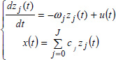
Consider the linear FDS in the Laplace domain:

corresponding to the following FDS:
Its integer order counterpart is defined with n1 = n2 = 1
4.2.2. Numerical simulation example
Simulation parameters are
Initial conditions are
in the integer order case, and
in the fractional order case.
The objective is to compute the input u(t) able to transfer x1(t) and x2(t) from their initial states at t = 0 to 0 at the instant tc with tc = 2kcTe.
The computation of u(t) is performed using a technique presented in section 4.4.6.
The graphs in Figure 4.1 present u(t), x1(t) and x2(t) for n1 = n2 = 1. We can verify that x1(t) = 0 and x2(t) = 0 whatever t ≥ tc, which is the usual property of state control in the integer order case.

Figure 4.1. ODE state control. For a color version of the figures in this chapter, see www.iste.co.uk/trigeassou/analysis2zip
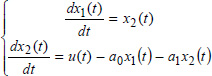
Similarly, u(t), x1(t) and x2(t) are presented in Figure 4.2. Although x1(tc) = 0 and x2(tc) = 0, we have to note that x1(t) ≠ 0 and x2(t) ≠ 0 for t > tc.
Figure 4.2. FDE pseudo-state control
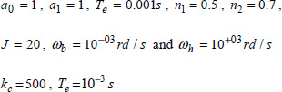
In order to explain this phenomenon, we present in Figure 4.3 the distributions of the internal states z1,j(t) and z2,j(t) at t = 0 and t = tc.
Figure 4.3. Distributions of FDE internal states
We note that the distributions z1, j(t) and z2, j(t) are modified by the control input; however, we do not obtain z1, j(tc) = 0 and z2, j(tc) = 0 for each value of j (i.e. ∀ ω), which would be the necessary condition to obtain x1(t) = 0 and x2(t) = 0 for t > tc.
We can conclude that the true control of fractional system state requires the control of all the frequency modes of the distributed states z1(ω, t) and z2(ω, t).
4.3. State control of the elementary FDE
4.3.1. Introduction
In the previous section, we demonstrated that the state control of an FDE requires the control of z(ω, t), which is the distributed state of the closed-loop representation.
This problem was briefly treated in Chapter 2 for controllability objectives. Let us recall that it is not possible to control z(ω, t) ∀ ω on a finite time interval. On the contrary, it is possible to control a finite dimension approximation Ẕ(t) on a finite time interval.
Therefore, our objective is to propose a methodology to control the frequency discretized modes Ẕ(t) of an elementary FDE. We demonstrate that the main problem is the state control of the associated fractional integrator.
4.3.2. State control of a fractional integrator
4.3.2.1. Problem statement
Let us consider the fractional integrator ![]() , which is characterized by the distributed state z(ω, t), excited by an input u(t).
, which is characterized by the distributed state z(ω, t), excited by an input u(t).
More precisely, we consider its finite dimension approximation zj(t) (see Chapter 2 of Volume 1) such as
The system [4.7] is in fact a large dimension integer order system (dim Ẕ(t) = J + 1):


Now consider a time discretization of [4.8] with the sample period Tce.
Then
REMARK 1.–
- – j is the frequency index and k is the time index.
- – For simulation purposes, Te is the time increment, which has to be chosen very small in relation to ωh. On the contrary, the sample period Tce for state control has to be adapted to the time response of the system.
- – Therefore, in practice, Tce ≫ Te such as
Tce = kcTe with kc ≫ 1
Consider the standard problem: calculate u(t) for t ∈ [0, tf], allowing the transfer of Ẕ(t) from an initial value Ẕ(0) to any final state Ẕ(tf).
Therefore, it is necessary to compute J + 1 values uj(t) of the input, i.e.
with tf = (J + 1)Tce
The different steps of the calculation are

Therefore
which corresponds to
where ![]() is the controllability matrix (Chapter 2).
is the controllability matrix (Chapter 2).
Thus, the control input ![]() is the solution of
is the solution of
The calculation of the (J + 1) components of the finite dimension approximation of z(ω, t) is not a new problem: fundamentally, it corresponds to the calculation of the input of an integer order differential system, which is a well-known problem.
However, let us specify the composition of the matrix ![]() .
.
Therefore, recall that system [4.8] is decoupled. Thus, we can express F and ![]() as
as
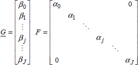
with

Therefore, the matrix ![]() corresponds to
corresponds to

Consider the components of ![]() ; note that frequencies ωj vary from ωj = 0 to ωj → ∞.
; note that frequencies ωj vary from ωj = 0 to ωj → ∞.
If ωj → ∞, then
On the contrary, if ωj → 0, then
Concretely, the matrix ![]() corresponds to
corresponds to

Theoretically, the matrix ![]() is invertible since the system [4.8] is diagonal. Practically, this matrix is very ill-conditioned for a conventional numerical technique [NOU 91], due to the very wide spectrum of ωj values.
is invertible since the system [4.8] is diagonal. Practically, this matrix is very ill-conditioned for a conventional numerical technique [NOU 91], due to the very wide spectrum of ωj values.
We can conclude that the state control of a fractional integrator is not a conventional problem. It requires a specific approach, as in the case of the initialization problem.
4.3.2.2. Solving a linear system with a recursive least-squares algorithm
Consider the linear system
The solution ![]() is equal to
is equal to
if A is invertible.
A necessary condition is
However, this condition is not sufficient.
Let λi (i = 1 to N) be the eigenvalues of A. The conditioning of the matrix A , i.e. its ability to be inversed, is characterized by [MOK 97]

A well-conditioned matrix is characterized by
A high value of cond(A) indicates bad conditioning.
In the case of ![]() (equations [4.17] and [4.20]), we have cond(A) → ∞, i.e. it is impossible to compute
(equations [4.17] and [4.20]), we have cond(A) → ∞, i.e. it is impossible to compute ![]() .
.
There are different techniques [MAR 93, MOK 97] adapted to ill-conditioned matrices and linear systems; however, they do not correspond to the problem of ![]() inversion.
inversion.
Thus, we later propose an inversion technique based on the recursive least-squares method, avoiding ![]() inversion.
inversion.
Let ![]() be an estimation of
be an estimation of ![]() , verifying [4.21].
, verifying [4.21].
Let us define the estimation error
and consider the quadratic criterion
The value ![]() minimizing J corresponds to
minimizing J corresponds to

As
we obtain
As
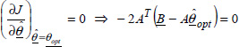
Thus
REMARK 2.– Let us multiply [4.21] by AT. Therefore, we obtain an equivalent solution
which is the optimal least-squares solution [4.32].
Thus, the least-squares solution [MEN 73, LJU 87] is also the solution of the linear system [4.21].
Nevertheless, solution [4.32] is not interesting because it also requires a matrix inversion.
Recall that there exists a recursive solution to the identification of transfer function models called the recursive least-squares (RLS) algorithm [NOR 86].
Let
be the linear in the parameter model (LP model).
Let us define
and
where ![]() is the measurement of yk, and
is the measurement of yk, and ![]() is its estimation based on
is its estimation based on ![]() (for k = 1 to K).
(for k = 1 to K).
The solution ![]() minimizing JK is given by [NOR 86]
minimizing JK is given by [NOR 86]
Then, for K measurements, let us define
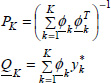
Therefore
Obviously, for K – 1 measurements
Then, replace K with k, i.e. we decide to compute ![]() at each instant k: the RLS algorithm provides the recursive estimation value
at each instant k: the RLS algorithm provides the recursive estimation value ![]() based on the previous knowledge
based on the previous knowledge ![]() , Pk – 1, as follows [NOR 86, LJU 87]:
, Pk – 1, as follows [NOR 86, LJU 87]:
where ![]() is an adaptive gain and
is an adaptive gain and
Normally, the solutions [4.40] and [4.41] appear to be more complex than [4.32].
Note that ![]() is a scalar; hence,
is a scalar; hence, ![]() is an elementary calculation.
is an elementary calculation.
Consequently, with algorithms [4.40] and [4.41], we can recursively compute the solution ![]() with K iterations, avoiding matrix inversion required by [4.32].
with K iterations, avoiding matrix inversion required by [4.32].
However, the solution ![]() depends on the initial estimation
depends on the initial estimation ![]() and the matrix P0: how should these initial values be chosen?
and the matrix P0: how should these initial values be chosen?
Note that Pk is related to the covariance matrix of ![]() , i.e. the confidence related to estimation
, i.e. the confidence related to estimation ![]() [LJU 87].
[LJU 87].
A good confidence in ![]() corresponds to small values of Pk. On the contrary, no confidence in
corresponds to small values of Pk. On the contrary, no confidence in ![]() is equivalent to large values of Pk.
is equivalent to large values of Pk.
At the limit, if there is no information on ![]() and P0, we have to use
and P0, we have to use ![]() and P0 = α I with α ≫ 1.
and P0 = α I with α ≫ 1.
Finally, note that K ≫ N corresponds to the case of recursive identification. However, at the limit, we can use K = N, where ![]() : of course, this would be a very bad solution for an identification problem with noisy data! However, this is a way to compute the solution of an ill-conditioned problem.
: of course, this would be a very bad solution for an identification problem with noisy data! However, this is a way to compute the solution of an ill-conditioned problem.
Before using [4.40] and [4.41] for the computation of [4.14], we propose to perform numerical simulations to test the influence of the different parameters on the solutions [4.40] and [4.41] when K = N.
4.3.2.3. A numerical example
Consider the elementary example
with
The matrix A is ill-conditioned since cond(A) = 23.1.
We impose
Thus, the equality ![]() leads to
leads to
Then, using algorithms [4.40] and [4.41], we obtain the successive estimations ![]() .
.
In order to objectively judge the quality of ![]() , we use the quadratic criterion
, we use the quadratic criterion
Therefore, with ![]() and α = 103, we obtain
and α = 103, we obtain

![]() is close to
is close to ![]() , but there are remaining errors.
, but there are remaining errors.
Obviously, we can improve the estimations with a new recursion, initialized by ![]() and P3.
and P3.
Therefore, we obtain

There is an improvement, but the convergence is too slow. Another solution is to increase P0, i.e. α.
Let α = 1010; we obtain

Thus, with a large value of α, only one recursion is required to obtain ![]() .
.
4.3.2.4. State control of the fractional integrator using the RLS algorithm
We have previously demonstrated that the control input ![]() , which allows the transfer of the internal state Ẕ from an initial value Ẕ(0) to any final value Ẕ(tf), is given by equations [4.40] and [4.41].
, which allows the transfer of the internal state Ẕ from an initial value Ẕ(0) to any final value Ẕ(tf), is given by equations [4.40] and [4.41].
Thereafter, we are interested in the standard case Ẕ(tf) = 0 with tf = (J + 1)Tce.
Therefore, the control input ![]() has to satisfy
has to satisfy
This equation can be decomposed into J+ 1 lines.
For line j, we can write

which corresponds, with the RLS notation, to
Therefore, we can recursively compute the control input ![]() with the RLS algorithm, starting from
with the RLS algorithm, starting from ![]() with P0 = α I.
with P0 = α I.
Index j varies from 1 to J + 1:
with

The quality of the estimation ![]() is characterized by the criterion
is characterized by the criterion
This criterion depends on α as ![]() depends on α.
depends on α.
Moreover, we can characterize the achieved control input ![]() by its “energy” criterion
by its “energy” criterion
Let us recall that in contrast to the elementary example 4.3.2.3, it is impossible to know the “true” value of ![]() because
because ![]() . Thus, the criterion Jz(α) is the only way to appreciate the quality of estimation
. Thus, the criterion Jz(α) is the only way to appreciate the quality of estimation ![]() .
.
4.3.2.5. Computation of a control input example
Consider the fractional integrator ![]() with
with
The integrator is simulated with the usual parameters
The sample period for the control input ![]() is
is
In order to use a realistic initial condition, we perform an initialization simulation with
The input uinit(t) and the response xinit(t) are presented in Figure 4.4.
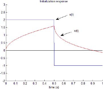
Figure 4.4. Initialization procedure
The final distributed state Ẕ of this simulation is used as an initial condition for the computation of control input ![]() in the interval [0, Tce(J + 1)].
in the interval [0, Tce(J + 1)].
The corresponding graphs of ![]() and x(t) (for α = 106) are presented in Figure 4.5; the corresponding distributions of Ẕ(0) and Ẕ(tf) are presented in Figure 4.6.
and x(t) (for α = 106) are presented in Figure 4.5; the corresponding distributions of Ẕ(0) and Ẕ(tf) are presented in Figure 4.6.
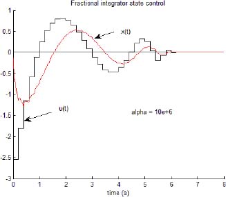
Figure 4.5. Fractional integrator state control
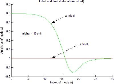
Figure 4.6. Initial and final distributions of the internal state
We obtain Jz(α) = 7.7E–06 and Ju(α) = 3.18.
A new computation of ![]() is performed with α = 108.
is performed with α = 108.
We obtain Jz(α) = 3.2E–07 and Ju(α) = 14.1.
The conclusion is that Ẕ(tf) is closer to 0, but at the same time, the control input ![]() is more “energetic” than previously.
is more “energetic” than previously.
In order to appreciate the influence of α on Jz(α) and Ju(α), we repeat the computation of ![]() for increasing values of α (see Table 4.1).
for increasing values of α (see Table 4.1).
Table 4.1. Influence of α
| α | 104 | 106 | 108 | 1010 | 1012 | 1014 | 1016 |
| JZ(α) | 1.7E–4 | 7.7 E–6 | 3.2E–7 | 1.6E–8 | 1.8E–9 | 2.7E–9 | 2.1E–7 |
| Ju(α) | 0.72 | 3.18 | 14.1 | 62.5 | 188.3 | 774 | 6350 |
Jz(α) is minimum for α = 1012, while Ju(α) regularly increases with α. A compromise is necessary between precision and control input energy. For example, α = 106 or α = 108 seem to be an acceptable compromise.
There is another parameter with a great influence on û, i.e. the sample period Tce. With Tce varying from 100ms to 400ms, with α = 108, we obtain the following values of Jz(α) and Ju(α) (see Table 4.2).
Table 4.2. Influence of Tce
| Tce (s) | 0.1 | 0.2 | 0.3 | 0.4 |
| JZ(α) | 5.9E–6 | 3.2E–7 | 6.7E–8 | 2.5E–8 |
| Ju(α) | 81.1 | 14.1 | 5.5 | 3.0 |
4.3.2.6. Conclusion
This numerical simulation has shown the main features of the proposed methodology for the state control of the fractional integrator. The RLS algorithm makes it possible to compute the control input ![]() ; however, the result is not unique. It depends on the initialization parameter α : with the criterion Jz(α), we can appreciate the precision of numerical computation.
; however, the result is not unique. It depends on the initialization parameter α : with the criterion Jz(α), we can appreciate the precision of numerical computation.
However, a “better” control input ![]() corresponds to an increase in control input “energy”. Moreover, for an imposed value of α, Jz(α) and Ju(α) decrease when the sample period Tce is increased.
corresponds to an increase in control input “energy”. Moreover, for an imposed value of α, Jz(α) and Ju(α) decrease when the sample period Tce is increased.
The compromise Jz(α)/Ju(α) depends on α and Tce; thus, the user is confronted with an optimization problem with a constraint on the “energy” of the control input.
4.3.2.7. State control of a one-derivative FDE
We are interested in the state control of the fractional integrator because this operation is fundamental for the state control of the closed-loop representation of a fractional system.
Let us recall the simulation graph for a one-derivative FDE, where u(t) is the input of the fractional integrator (Figure 4.7) and uc(t) is the input of the FDE.

Figure 4.7. State control of a one-derivative FDE
This graph corresponds to the equation
Previously, we calculated the control input ![]() , allowing the transfer of Ẕ(t) from any initial state Ẕ(0) to an arbitrary final state Ẕ(tf). When we apply the control input
, allowing the transfer of Ẕ(t) from any initial state Ẕ(0) to an arbitrary final state Ẕ(tf). When we apply the control input ![]() to
to ![]() , we can compute Ẕ(t) and x(t), where
, we can compute Ẕ(t) and x(t), where
Using equation [4.60], with the knowledge of ![]() and x(t), we can compute the control input uc(t) applied to the FDE, allowing the transfer of its state Ẕ(t) from Ẕ(0) to Ẕ(tf) (since the integrator state is also the FDE state).
and x(t), we can compute the control input uc(t) applied to the FDE, allowing the transfer of its state Ẕ(t) from Ẕ(0) to Ẕ(tf) (since the integrator state is also the FDE state).
Therefore
Consider the control input ![]() corresponding to
corresponding to
Then, if we consider the system
we obtain the control input uc(t) (with [4.62]) presented in Figure 4.8 and the corresponding output x(t), which corresponds exactly to x(t), presented in Figure 4.5.

Figure 4.8. FDE state control
4.4. State control of an FDS
4.4.1. Introduction
The objective of this section is to propose a methodology for the state control of the distributed state Ẕ(ω, t) (in fact, a finite dimensional discretization Ẕ) of a non-commensurate order system
However, we restrict the class of FDSs to the non-commensurate order FDEs represented by the transfer function
corresponding to the simulation graph of Chapter 1 of Volume 1, where the integrators ![]() are connected in series, as a generalization of the elementary case considered previously.
are connected in series, as a generalization of the elementary case considered previously.
For a single integrator, the system matrix A is diagonal.
Thus, it is possible to explicitly formulate the relations between Ẕ(t) and the coefficients αi and βj.
For an integrator chain, the composition of matrix A is more complex due to the couplings between the integrators imposed by the relations ui(t) = xi+1(t).
Therefore, we present thereafter a general formulation of the relation ![]() depending on Asys and Ḇsys.
depending on Asys and Ḇsys.
Practically, this relation will be used for the two-integrator case.
4.4.2. Principle of state control
Remember that the objective is not the state control of Ẕ(ω, t), which would require an infinite control time, but the state control of a finite dimensional approximation Ẕ(t) defined as
Where
Each integrator ![]() characterized by the state model:
characterized by the state model:
with the constraint
For the whole system, the state space model is
Knowledge of the matrices Asys and Ḇsys enables us to determine the matrices F and ![]() corresponding to the discrete state-space representation [4.71] for the sample period Tce thanks to standard algorithms available in mathematical solvers [MOK 97].
corresponding to the discrete state-space representation [4.71] for the sample period Tce thanks to standard algorithms available in mathematical solvers [MOK 97].
Then, we can write
We previously demonstrated that the control input {uk} for a single integrator with J + 1 modes must be composed of J + 1 terms, varying from u0 to uJ.
For an integrator chain composed of N elements, each one with J + 1 modes, the control input {uk} will be composed of N(J + 1) terms, varying from u0 to uJmax with Jmax = N (J + 1) –1.
Therefore, the explicit system of equations based on u0 to uJmax is

corresponding to
with
i.e.
where ![]() is the controllability matrix (Chapter 2).
is the controllability matrix (Chapter 2).
The control input ![]() allows the transfer of Ẕ(t) from any initial value Z(0) to the final value Ẕ(tf) with tf = Tce(Jmax + 1).
allows the transfer of Ẕ(t) from any initial value Z(0) to the final value Ẕ(tf) with tf = Tce(Jmax + 1).
The control input ![]() is provided by
is provided by
As mentioned previously, the control input ![]() is recursively computed using the RLS algorithm [4.40] and [4.41].
is recursively computed using the RLS algorithm [4.40] and [4.41].
4.4.3. State control of two integrators in series
Consider the series system in Figure 4.9.
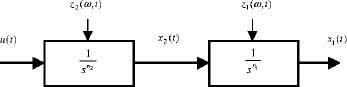
Figure 4.9. Two fractional integrators in series
The integrators ![]() and
and ![]() are characterized by the state equations
are characterized by the state equations

Let us define
Then

With

Therefore

The Z-transform [KRA 92], with the sampling time Tce, provides the matrices ![]() of the discrete state equations.
of the discrete state equations.
Thus, we can write
This linear system is composed of Jmax+ 1 lines from j = 1 to Jmax+1.
Consider the standard case Ẕ(tf) = 0.
Let us define fj(0) as the component j of the product FJmax+1Ẕ0 and ![]() as the line j of the matrix
as the line j of the matrix ![]() .
.
Then, the line j of equation [4.83] corresponds to
The control input ![]() is provided by the minimization of the quadratic criterion
is provided by the minimization of the quadratic criterion
4.4.4. Numerical example
Consider the following example
ωh = 10+3rd / s, ωb = 10–3rd / s and J = 30 for each integrator and Tce = 300ms.
The initial state  is provided by the simulation of the corresponding FDE (see Figure 4.10).
Ẕ1(0) and Ẕ2(0) are plotted in Figure 4.12.
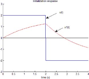
Figure 4.10. Initialization procedure
The control input ![]() is computed using the RLS algorithm with α = 1010.
is computed using the RLS algorithm with α = 1010.
The graphs of u(t), x1(t) and x2(t) are presented in Figure 4.11; the distributions of Ẕ(0) and Ẕ(t) are presented in Figure 4.12.

Figure 4.11. State control of two fractional integrators in series
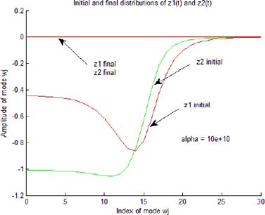
Figure 4.12. Distribution of initial and final internal states
For α = 1010, we obtain
As discussed previously, we test the influence of Tce for α = 1010 (see Table 4.3).
Table 4.3. Influence of Tce
| Tce (s) | 0.1 | 0.2 | 0.3 | 0.4 |
| JZ(α) | 1.8E–5 | 3.2 E–7 | 3.6 E–8 | 1.3E–8 |
| Ju(α) | 14000 | 670 | 106 | 28 |
We note that the increase of Tce allows a better precision and a lower “energy” of the control input.
4.4.5. State control of a two-derivative FDE
Consider the FDE
Using the previous control input u(t), we can express the FDE control input uc(t), allowing the transfer of Ẕ(t) from Ẕ(0) to Ẕ(tf).
Using
we can compute uc(t) for t ∈ [0, tf] thanks to the equation
Consider the previous example with the same parameter values (a0 = 1 a1 =1). The corresponding graphs of u(t), x1(t) and x2(t) are presented in Figure 4.13.

Figure 4.13. Two-derivative FDE state control
4.4.6. Pseudo-state control of the two-derivative FDE
In section 4.2, it was highlighted that the control of the pseudo-states x1(t) and x2(t) does not allow the true state control of the two-derivative FDE. However, we did not express the calculation of uc(t), allowing the transfer of the pseudo-state  from an initial state, i.e.
  with tc = 2Tce.
First, we calculate  .
.
Using equation [4.83], we can write
Using [4.82], we obtain
i.e.
Thus
In this case, matrix inversion is easy. Then, with u(t), we compute Ẕ1(t) and Ẕ2(t), and therefore x1(t) and x2(t) using [4.82].
Finally, we can compute the control input uc(t) thanks to [4.90].
4.5. Conclusion
This chapter was dedicated to the state control of fractional integrators with application to the state control of fractional order differential systems. The objective was not to propose a new control strategy but to highlight the specificities and the difficulties of FDS state control. Numerical examples were proposed to illustrate all these features, without an application objective.
This methodology is an open-loop approach to state control or feed-forward state control. The corresponding practical methodology would be a closed-loop approach to feedback state control, based on the principles highlighted previously.
Moreover, we demonstrated the necessary compromise between state accuracy and control “energy”, corresponding to an optimization problem with constraints. The next step would be the optimal control of the internal distributed state, but it is out of the scope of our objective in this book. However, in the next chapter, we present an application to the control of a diffusive system in order to demonstrate the interest of FDS state control.