9
Lyapunov Stability of Non-commensurate Order Fractional Systems
9.1. Introduction
In the previous chapter, it has been demonstrated that the Lyapunov stability of commensurate fractional order systems is closely related to the stability of integer order systems, as they are commensurate order systems with n = 1, nevertheless with important specificities. In spite of these constraints, it has been possible to express an LMI stability condition, thanks to the duality between closed-loop and open-loop representations.
The situation is completely different with non-commensurate fractional order systems corresponding to the general model:
Let us recall that matrix transformation or modal representation does not exist for these systems (see Chapter 2).
Therefore, it is not possible to formulate a Lyapunov function equivalent to
for at least three main reasons:
- – the weighting function µni((ω) depends on each fractional order ni;
- – it is not possible to formulate a weighting matrix P = (M–1)T M–1 > 0 since the matrix transformation
 does not exist;
 - – we cannot use the duality closed-loop/open-loop representation because partial fraction expansion cannot be used.
Thus, the Lyapunov stability of non-commensurate fractional order systems, expressed by an LMI condition, is (up to our knowledge) a non-solved complex problem.
In this chapter, we propose a different approach that is based on an energy formulation of the Lyapunov function. The Lyapunov stability of commensurate order systems has partially used the characteristics of the energy stored in the fractional integrators. In particular, dissipation of this energy has not been used explicitly (see Chapter 7).
Thus, in this chapter, our objective is to use the specific features of fractional energy, such as storage and dissipation, to express the stability condition of electrical systems thanks to an energy balance principle. Let us recall that it is not an original methodology. It has already been used in the theory of passivity to formulate control laws for electromechanical nonlinear systems, such as electrical machines, robots manipulators and so on [ORT 98].
In the first step, it is necessary to express the energy stored in fractional order electrical devices, such as capacitors and inductors. Although these concepts can be generalized to other systems such as mechanical, chemical or biological ones, we limit this approach to electrical systems because it is easy to define such fractional devices.
The classical RLC series circuit will be used to recall that its stability condition is closely related to the energy balance principle. Then, it will be possible to analyze the Lyapunov stability of more complex systems, in terms of energy balance, and also using dissipation and regeneration of energy [TRI 16a]. Finally, the LMI stability condition of commensurate order systems (analyzed in Chapter 8) will be revisited and interpreted in terms of energy balance and dissipation of energy [TRI 16b].
9.2. Stored energy, dissipation and energy balance in fractional electrical devices
9.2.1. Usual capacitor and inductor devices
Let us recall that a capacitor C is characterized by the equation (see Figure 9.1)
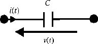
Figure 9.1. Capacitor circuit
The electrostatic energy stored in the capacitor is expressed as [JOO 86, IRW 99]
Using the Laplace transform, equation [9.3] becomes
Therefore
where
is the complex impedance of the capacitor.
Similarly, for an inductor L (see Figure 9.2), we can write [IRW 99]
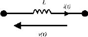
Figure 9.2. Inductor circuit
The magnetic energy stored in the inductor is expressed as
We can also write
or
where
is the complex impedance of the inductor.
Capacitor C and inductor L are the only elementary electrical devices able to store energy. On the contrary, they do not dissipate energy, at least in their idealized form.
9.2.2. Fractional capacitor and inductor
Let us now consider electrical complex devices such as RC and RL infinite length lines. The RC line has already been analyzed to investigate some properties of the fractional integrator (see Chapter 6 of Volume 1). The RL line can also be modeled as a fractional order system (see Appendix A.9.1).
These devices can be interpreted as realizations of the fractional integrator and of the fractional differentiator. However, they can also be interpreted as fractional capacitors and inductors.
9.2.2.1. Fractional capacitor
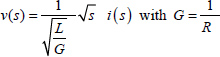
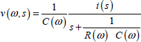
For the infinite length RC line (see Chapter 6 of Volume 1), we demonstrated that (see Figure 9.3)
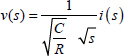
Let us define
then
where
Thus
which is the fractional generalization of
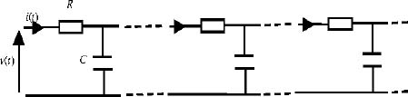
Figure 9.3. Infinite length RC line
9.2.2.2. Fractional inductor
It is demonstrated in Appendix A.9.1 that the infinite length RL line (or GL line as shown in Figure 9.4) is characterized by
Let us define
then
where
Thus
which is the fractional generalization of
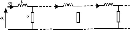
Figure 9.4. Infinite length GL line
9.2.3. Energy storage and dissipation in fractional devices
9.2.3.1. Fractional capacitor
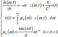
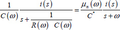
A distributed model with the internal variable zC(ω, t) is associated with the electrical equation i(t) = C*Dn (v(t)) (see Chapter 7).
Therefore
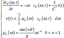
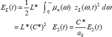
The energy stored in the fractional capacitor C* is expressed (see Appendix A.9.2) as
In contrast to the usual capacitor, an electrical power P(t) is also dissipated in the fractional capacitor.
It is expressed as
The energy is stored in the distributed capacitors C and dissipated in the distributed resistors R of the infinite length RC line.
9.2.3.2. Fractional inductor
A distributed model with the internal variable zL(ω, t) is associated with the electrical equation v(t) = L*Dn(i(t)).
Therefore
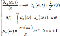
Similarly to the fractional capacitor, the energy stored in the fractional inductor L* is expressed as [HAR 15b]
and the electrical power dissipated in the fractional inductor is expressed as:
9.2.3.3. Passive circuits, active circuits
Passive electrical circuits are composed of capacitors, inductors and resistors. Energy storage devices are capacitors and inductors, whereas resistors are dissipative devices.
Active electrical circuits are composed of passive devices (R, L and C) and of electronic systems performing complex and artificial functions.
In particular, using a positive feedback, it is possible to realize the equivalent of a negative resistor [AUV 80, CHA 82], which regenerates energy (instead of dissipating it).
This negative resistor is used in the usual LC oscillator in order to compensate the power dissipated in resistors and so to maintain a constant amplitude oscillation [CHA 82, KHA 96].
Negative resistors will be used to express the stability condition of fractional electrical circuits.
9.2.4. Reversibility of energy and energy balance
9.2.4.1. Reversibility and irreversibility of energy
Energy storage devices are capacitors and inductors. The energy stored either in capacitors or inductors is characterized by its reversibility [JOO 86]. In particular, capacitors and inductors can exchange their energies; it is what occurs in the LC oscillator.
During these transfers, energy is also dissipated in resistors where it is transformed into heat according to the Joule effect. Globally, for an isolated system with no external source of energy, the initial energy stored in C and L devices is completely transformed into heat in the resistors.
Let us recall that this transformation is irreversible; heat cannot be transformed again into any kind of electrical energy: heat is an irreversible energy [JOO 86].
This means that the methodology proposed in this section for electrical systems is strictly limited to reversible energies. Thermal phenomena are excluded, except for those related to dissipation in resistors. On the contrary, this methodology applies to mechanical systems, where energy can be stored in moving masses (kinetic energy) or in springs (potential energy) [JOO 86]. Similarly, energy transfers between masses and springs are transformed into heat by frictions, i.e. into irreversible energy, as in resistors.
9.2.4.2. Energy balance
Energy balance and conservation of energy are fundamental principles of physics [JOO 86, ORT 98].
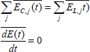
For an autonomous system, they state that, for energy transfers:
and for dissipated powers:
The term Ej(t) represents reversible energies such as kinetic, potential, magnetic or electrostatic energies for electromechanical systems. The term Pj(t) represents energy dissipation in resistors or frictions which is transformed into heat.
Equation [9.31] expresses conservation of energy or energy balance. Practically, this equation has to be adapted to systems where energy transfers are characterized by a periodical decreasing phenomenon. Thus, the derivative ![]() has to be replaced by the mean of the energy derivative, i.e. by
has to be replaced by the mean of the energy derivative, i.e. by  .
.
9.3. The usual series RLC circuit
9.3.1. Introduction
Although perfectly known, the energy transfers between an inductor L and a capacitor C provide the opportunity to propose a methodology to analyze the stability of fractional systems.
9.3.2. Analysis of the series RLC circuit
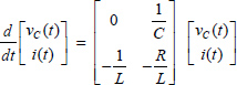
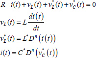
The series RLC circuit is presented in Figure 9.5. The components L and C are characterized by the equations
Moreover, R i(t) + vL(t) + vC(t) = 0.
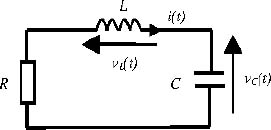
Figure 9.5. Series RLC circuit
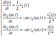
The state variables are vC(t) for C and i(t) for L. Therefore, the state space model of the circuit is
At t = 0, the initial conditions are vC(0) and i(0). The energies stored in L and C are expressed as
Thus, the global system energy (or Lyapunov function V(t)) is the sum of these two energies
and its derivative is
therefore:
This derivative expresses that energy is dissipated in resistor R.
Thus:
- – for R > 0, the system is stable;
- – for R < 0, the system is unstable.
Limit of stability occurs for R = 0 and a constant amplitude oscillation appears.
9.3.3. Stability analysis
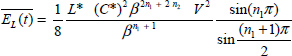
Of course, this stability analysis is trivial. However, let us consider the waveforms of EL(t), EC(t) and V(t) (see Figure 9.6) which are simulated with
The graphs of EL(t) and EC(t) are shifted damped sinusoids. Their sum V(t) is a monotonous decreasing function. For R = 0, these sine functions have a constant amplitude and their sum is a constant. These curves express that the energy EL(t) with the initial value ![]() is transferred to the capacitor, so EC(t) can increase. When EC(t) is maximum (and EL(t) minimum), a new cycle of energy transfer occurs, and so on. These exchanges between L and C are perfect with no loss when R = 0, i.e. when there is a perfect energy balance between the two components, with no dissipation.
is transferred to the capacitor, so EC(t) can increase. When EC(t) is maximum (and EL(t) minimum), a new cycle of energy transfer occurs, and so on. These exchanges between L and C are perfect with no loss when R = 0, i.e. when there is a perfect energy balance between the two components, with no dissipation.
When R = 0, let us define
Therefore
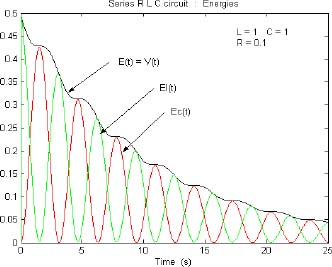
Figure 9.6. Energies of the series RLC circuit. For a color version of the figures in this chapter see, www.iste.co.uk/trigeassou/analysis2.zip
Thus
These functions have two components: a constant part, equal to their mean, and a time-varying part, the frequency of which is twice that of vC(t) or i(t).
The two means are equal because there is no loss in the resistor.
Therefore
Thus, the oscillation frequency is derived from the equality of the means of the two complementary energies EL(t) and EC(t):
Let us recall that the derivative ![]() provides the stability condition:
provides the stability condition: ![]() or R > 0.
or R > 0.
This is the energy balance principle, between complementary components, which will be used to derive stability conditions for fractional order systems.
9.4. The series RLC* fractional circuit
9.4.1. Introduction
The series RLC* fractional circuit is a typical non-commensurate order system, with n = 1 for L and 0 < n < 1 for C*. It allows a simple analysis of transients and energy transfers between L and C*.
9.4.2. Analysis of the series RLC* circuit
The series RLC* circuit corresponds to Figure 9.5, where capacitor C is replaced by C*. The components L and C* are characterized by the equations
Moreover, R i(t) + vL(t) + vC(t) = 0.
The state variables are i(t) for the inductor L and zC(ω, t) for the fractional capacitor C*.
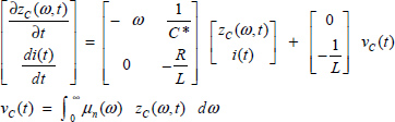
Therefore, the state space model of this circuit is
At t = 0, the initial conditions are zC(ω, 0) and i(0). The energies stored in L and C* are expressed as
Thus, the total system energy E(t) or the Lyapunov function V(t) is the sum of these two energies
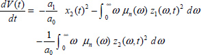
and its derivative is
Thus
This equation expresses that the energy V(t) is dissipated inside the fractional capacitor by internal Joule losses and outside in resistor R.
For R > 0 , the circuit is essentially dissipative and energy stored in L and C* can only decrease. Note that the damping is more important than in the previous RLC circuit thanks to internal Joule losses in C*.
However, an important difference has to be noted: for R < 0, the term –R i(t)2 is now positive, whereas the second term remains negative. Negative resistors are artificially provided by positive feedback circuits [AUV 80, CHA 82] or Tunnel diodes [KHA 96].
9.4.3. Experimental stability analysis
Numerical simulations are necessary to highlight some specific features of fractional systems. The RLC* circuit is simulated with
For the fractional integrator, J + 1 = 21, with ω varying from ωb = 0.001 rad/s to ωh = 1000 rad/s; Te = 10–3s.
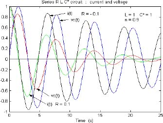
Figure 9.7. Current and voltage of the RLC* circuit
The waveforms of i(t) and vC(t) are presented in Figure 9.7 for R = 0.1 and R = –0.1. We can note that the circuit is of course stable for R = 0.1 and also for R = –0.1. Then, the graphs of V(t), EL(t) and EC(t) are presented in Figure 9.8 for R = 0.1 and in Figure 9.9 for R = –0.1.
Figure 9.8. Energy of the RLC* circuit, R = 0.1
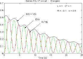
Figure 9.9. Energy of the RLC* circuit, R = –0.1
The decrease of V(t) is monotonous for R > 0, as noted for the integer order RLC circuit. On the contrary, an oscillation of V(t) appears for R < 0, i.e. we can observe a series of energy regeneration and dissipation phases.
This phenomenon is a specificity of fractional systems, and it has already been observed in the commensurate order case [TRI 13b, TRI 13c]. It is easily explained using the interpretation of ![]() .
.
The two components –Ri(t)2, ![]() and their sum
and their sum ![]() for R = –0.1 are presented in Figure 9.10.
for R = –0.1 are presented in Figure 9.10.
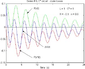
Figure 9.10. Derivative of the Lyapunov function
For R > 0 (Figure 9.8), the two components are negative, so ![]() and the decrease of V(t) is monotonous.
and the decrease of V(t) is monotonous.
On the contrary, for R < 0 (Figure 9.9), the two components have opposite signs and their sum is alternatively positive and negative. Consequently, V(t) (Figure 9.9) is globally decreasing, but its decrease is no longer monotonous but periodic.
For ![]() phases, V(t) is regenerated, whereas it is dissipated for
phases, V(t) is regenerated, whereas it is dissipated for ![]() phases.
phases.
This is not a new oscillating phenomenon: it is caused by the natural damped oscillation of i(t) and vC(t), combined with the effect of the –R i(t)2 term when R < 0 (see Figure 9.10).
Despite these oscillations, we can conclude that the mean of ![]() is negative when the system is stable.
is negative when the system is stable.
Thus, ![]() ensures stability; however, this mean cannot directly be used to derive stability conditions.
ensures stability; however, this mean cannot directly be used to derive stability conditions.
9.4.4. Theoretical stability analysis
As observed with the integer order RLC circuit, the components L and C* exchange their complementary stored energies: the system remains stable if the energy is globally decreasing, i.e. if ![]() . A constant amplitude oscillation occurs at the limit of stability, and the Lyapunov function V(t) is globally constant (when all transients have vanished), i.e. its average value is constant.
. A constant amplitude oscillation occurs at the limit of stability, and the Lyapunov function V(t) is globally constant (when all transients have vanished), i.e. its average value is constant.
We can equivalently express this property using the energy balance principle applied to the means of the complementary energies EL(t) and EC(t).
Thus, at the limit of stability:
Moreover,
Recall that ![]() ensures stability.
ensures stability.
9.4.4.1. Derivation of oscillation frequency
Let us define vC(t) = Vej β t at the limit of stability, where β is the oscillation frequency.
As i(t) = C*Dn(vC(t)), we can write
We have to calculate ![]() . Recall that
. Recall that ![]() .
.
Thus
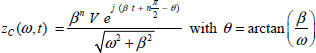
The calculation of ![]() requires zC(ω, t).
requires zC(ω, t).
According to (9.46), we obtain
with
thus
As ![]() , we obtain
, we obtain
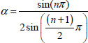
According to Appendix A.9.3, we can write
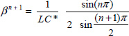
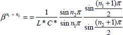
Consequently, the equality ![]() provides the value of β:
provides the value of β:
9.4.4.2. Stability condition
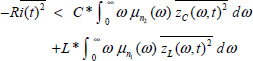
The circuit remains stable if ![]() . According to [9.50], this condition is equivalent to
. According to [9.50], this condition is equivalent to
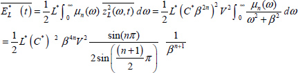
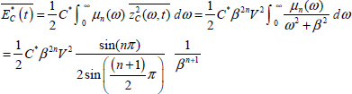
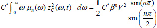
This condition expresses that the circuit remains stable if the mean of energy regeneration is less than the mean of internal Joule losses in the fractional capacitor. Unfortunately, these means are not easily calculated in the general case. However, at the limit of stability, it is straightforward to write
and
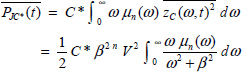
According to Appendix A.9.3
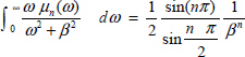
thus
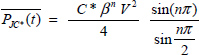
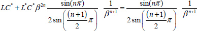
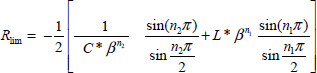
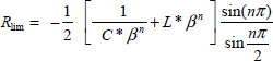
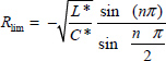
Consequently, we can deduce the limit value of R:
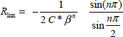
and stability is ensured if R > Rlim.
9.4.4.3. Example
The case n = 0.5 simplifies calculations. Moreover, it corresponds to the practical case of the infinite RC line (section 9.2.2.1). Note that this result can be verified using Matignon’s criterion (Appendix A.8.2).
As n = 0.5, we obtain
Thus
and
With L = 1 C* = 1, we obtain
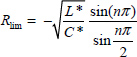
and stability is ensured if
9.4.5. Conclusion
Energy balance is a fundamental principle of physics [JOO 86, ORT 98]. For an autonomous system, it states that
As demonstrated by previous numerical simulations, the application of this principle to fractional systems has required important adaptations. More specifically, because ![]() is no longer a monotonous decreasing function, it cannot be used to characterize the stability of fractional systems.
is no longer a monotonous decreasing function, it cannot be used to characterize the stability of fractional systems.
Practically, we have to replace the derivative of energy by its mean because it remains a globally decreasing function. Therefore, the stability of a fractional system is characterized by
However, this mean is easy to calculate only at the limit of stability.
Consequently, the energy balance principle of an electrical fractional system has been defined at the limit of stability as
where
and V(t) is the system’s Lyapunov function.
9.5. The series RLL*C* circuit
9.5.1. Circuit modeling
The previous methodology is now applied to a more complex system in order to demonstrate its generality.
Consider the RLL*C* series circuit presented in Figure 9.11, which is governed by the following equations:
The state variables i(t), zC(ω, t) and zL(ω, t) are defined as
with
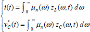
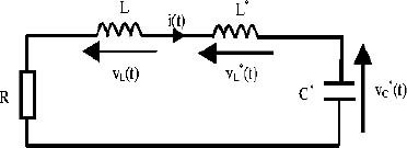
Figure 9.11. Series RLL*C* circuit
The corresponding energies are
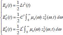
Thus
and
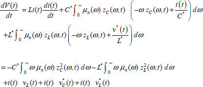
As ![]() , we obtain
, we obtain
As mentioned previously, ![]() is the sum of internal and external losses.
is the sum of internal and external losses.
If R > 0, the system is naturally damped.
9.5.2. Stability analysis
9.5.2.1. Oscillation frequency
When the circuit is at the limit of stability, i(t), ![]() ,
, ![]() and vL(t) are sine functions.
and vL(t) are sine functions.
Let us define ![]() .
.
As ![]() , we can write
, we can write
Then, according to [9.79]
As ![]() , we obtain
, we obtain
According to [9.79]
The frequency β is derived from the equality of the means of magnetic and electrostatic energies
therefore
and
Equation [9.90] corresponds to
Let
According to [9.94], the frequency β is the solution of the equation
In the particular case n = 0.5 , the frequency β is the solution of
Let β0.5 = X, then X is the solution of
9.5.2.2. Stability condition
The stability condition is derived from
As demonstrated previously
and
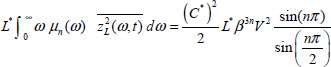
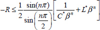
Then, R is derived from the inequality
or equivalently
9.6. The series RL*C* fractional circuit
9.6.1. Introduction
The series RL*C* fractional circuit is a typical non-commensurate order system, with two orders n1 for L* and n2 for C*. The particular case n1 = n2 = n will be used to formulate a new interpretation to the Lyapunov stability of commensurate order FDEs.
9.6.2. Analysis of the series RL*C* circuit
The series RL*C* circuit corresponds to Figure 9.12.
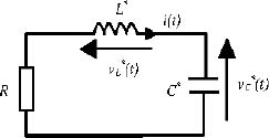
Figure 9.12. Series RL*C* circuit
The components L* and C* are characterized by the equations
Moreover
The state variables are zL(ω, t) for the inductor L* and zc(ω,t) for the capacitor C*. Therefore, the state space model of this circuit is
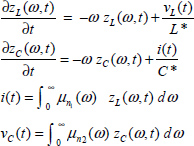
At t = 0, the initial conditions are zL(ω, 0) and zC(ω, 0). The energies stored in L* and C* are expressed as
Thus
and its derivative is
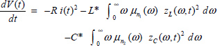
The last two terms represent internal losses in L* and C*, whereas the first one corresponds to external losses in R.
Therefore, as the system is naturally damped by all these losses, instability can occur only with an artificial negative resistor used to regenerate energy.
9.6.3. Theoretical stability analysis
The components L* and C* exchange their complementary stored energies: the system remains stable if the initial energy is globally decreasing, i.e. if ![]() .
.
Stability conditions are derived from the energy balance principle.
9.6.3.1. Derivation of oscillation frequency
At the limit of stability, when a constant oscillation occurs, we obtain
Then, let us define vC(t) = V ej β t, where β is the oscillation frequency.
As i(t) = C* Dn2 (vc(t)), we can write
and as vL(t) = L* Dn1 (i(t))
According to [9.107]
with
We have to calculate ![]() and
and ![]() .
.
Using the same technique as mentioned previously, we obtain
and
Consequently, the equality ![]() provides the value of β
provides the value of β
9.6.3.2. Stability condition
The circuit remains stable if ![]() . According to [9.111], this condition is equivalent to
. According to [9.111], this condition is equivalent to
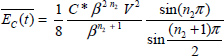
As ![]() at the limit of stability, we obtain
at the limit of stability, we obtain
and stability is ensured if
9.6.3.3. Commensurate order case
If n1 = n2 = n
Since
we obtain
9.7. Stability of a commensurate order FDE: energy balance approach
9.7.1. Introduction
Previously, it has been demonstrated that the stability analysis of the commensurate order RL*C* circuit can be derived from the energy balance approach. Equivalently, the stability analysis of any two-derivative commensurate order FDE can be derived from the analysis of an arbitrary fictitious RL*C* circuit.
9.7.2. Analysis of the commensurate order FDE
The series RL*C* commensurate order circuit corresponds to the simplified equations
The equation R i(t) + vL(t) + vC(t) = 0 is equivalent to the FDE
i.e.
with ![]() and
and ![]() .
.
This commensurate order FDE is simulated with two fractional integrators ![]() according to Figure 9.13.
according to Figure 9.13.
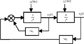
Figure 9.13. Simulation of a two-derivative FDE
The two infinite state variables are z1(ω, t) and z2(ω, t) such as
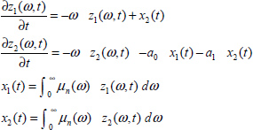
Of course
Therefore, z1(ω, t) = zC(ω, t) and ![]() , where zc(ω, t) and zL(ω, t) have been defined previously.
, where zc(ω, t) and zL(ω, t) have been defined previously.
Let us define
Then
Thus
Knowledge of R, L* and C* allows the definition of ![]() and
and ![]() . However, reciprocally, knowledge of a0 and a1 does not allow the complete definition of R, L* and C* since
. However, reciprocally, knowledge of a0 and a1 does not allow the complete definition of R, L* and C* since ![]() and R = a1 L*.
and R = a1 L*.
Therefore, it is necessary to make an arbitrary choice for one of the components, for example C*.
Then, we obtain
Consequently, the Lyapunov function is defined arbitrarily, depending on the choice of C*.
9.7.3. Application to stability
Let C* = 1, then
Thus
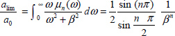
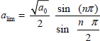
At the limit of stability
Let us define
Thus
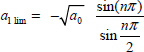
Therefore, a1 lim corresponds to the FDE stability condition derived from Matignon’s criterion (Appendix A.8.2). However, it is important to note that the previous arbitrary choice for C* has no consequence on the stability condition of [9.129].
This result means that the stability condition of any FDE as [9.129] can be derived from the energy balance principle, with arbitrary values of the fictitious series RL*C* circuit. Oscillations can be interpreted as transfers between electrostatic energy stored in the arbitrary capacitor C* and magnetic energy stored in L*. Moreover, damping is caused by internal losses in C* and L* and external losses in R.
9.8. Stability of a commensurate order FDE: physical interpretation of the usual approach
9.8.1. Introduction
The usual approach to stability analysis of a commensurate order system (either integer or fractional order) is to use a positive P matrix to weight the Lyapunov function (see Chapter 8). Fundamentally, it will be demonstrated that this weighting matrix technique is equivalent to the previous approach based on a fictitious arbitrary RL*C* circuit.
9.8.2. Commensurate order system
Consider the commensurate fractional order system
This system corresponds to the commensurate order FDE
which is simulated according to Figure 9.13. Its equivalence with the series RL*C* circuit has been demonstrated previously.
The eigenvalues λ1 and λ2 of A are the roots of the equation
Let a0 > 0
- – Δ > 0 if a1 < –2 a0 or a1 > 2 a0, then λ1 and λ2 are real eigenvalues.
- – Δ < 0 if –2 a0 < a1 < 2a0, then λ1 and λ2 are complex eigenvalues λi = a ± j b with:
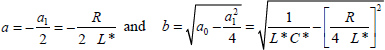
or λi = ρ e± j θ with
9.8.3. Lyapunov function of a fractional differential system
As system [9.143] is a commensurate order system, a modal representation can be associated with it. Let λi be the N eigenvalues of A in the general case. Let M be the matrix composed of the corresponding N eigenvectors (remember that M is not unique). Recall that
where Ad is the modal diagonal matrix.
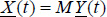
Consider the matrix transformation
N fractional integrators ![]() are associated with the modal pseudo-state variables yi(t), where wi(ω, t) are the internal variables (see Chapter 8):
are associated with the modal pseudo-state variables yi(t), where wi(ω, t) are the internal variables (see Chapter 8):
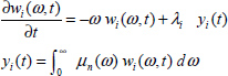
The energy of each modal integrator is
As the modal system [9.150] is composed of N independent modes, its total energy Vd(t) is the sum of the N independent energies Vi(t).
Therefore
Let us define
therefore
Then, consider the inverse transformation
As ![]() is also defined by [9.150], we obtain
is also defined by [9.150], we obtain
Therefore, we can write [9.154] as
Let us define (Chapter 8)
P is a symmetric definite positive matrix: there is an infinity of possibilities to define P depending on the choice of the eigenvectors of M.
As the matrix transformation [9.149] does not modify energy, the Lyapunov function V(t) of the N -derivative fractional system is defined as
9.8.4. Stability analysis
Consider the modal representation [9.150] with
9.8.4.1. Oscillation frequency
At the limit of stability, y1(t) and y2(t) are constant amplitude sine waveforms.
Let us define y1(t) = Y ej β t.
Then, y2(t) = Y e–j β t
and
therefore
and
Obviously, this result is the same as [9.140] derived from the energy balance approach.
9.8.4.2. Stability condition
with
At the limit of stability, ![]() .
.
Therefore, we have to calculate two means
Then
As
with ![]()
As
we obtain
Consequently
Thus, at the limit of stability, a = alim and
As ![]() ([9.140]), we obtain
([9.140]), we obtain
Recall that ![]() .
.
thus
The system remains stable if R > Rlim or a < alim, i.e. if
This last condition is equivalent to the LMI
where ![]() (see Chapter 8).
(see Chapter 8).
9.8.5. Conclusion
The previous analysis demonstrated that the usual approach to stability based on a weighted Lyapunov function is equivalent to the energy balance principle. Note that an LMI stability condition is derived from the usual approach, whereas a classical Routh stability condition is derived from the energy balance technique [ROU 77].
The standard FDE can be interpreted as a fictitious RL*C* circuit where the Lyapunov function is weighted by an arbitrary value of C*. Equivalently, the stability of the standard FDE can be analyzed with a Lyapunov function weighted by an arbitrary symmetric positive matrix P. This P matrix is related to the A matrix eigenvalues, i.e. to the arbitrary values of the fictitious RL*C* circuit. Consequently, the weighting matrix P can be interpreted in terms of a fictitious series RL*C* circuit.
According to [9.164], the term ![]() is equivalent to Joule losses in an external resistor R, whereas the term
is equivalent to Joule losses in an external resistor R, whereas the term ![]() represents internal Joule losses in the fractional integrators
represents internal Joule losses in the fractional integrators ![]() .
.
Finally, consider the general commensurate order fractional system
where
and
According to the previous analysis in the modal base and using the inverse transformation [9.155], the term ![]() can be interpreted as internal Joule losses in the N fractional integrators
can be interpreted as internal Joule losses in the N fractional integrators ![]() , whereas the other term
, whereas the other term ![]() can be interpreted as external Joule losses in fictitious resistors.
can be interpreted as external Joule losses in fictitious resistors.
A.9. Appendix
A.9.1. The infinite length LG line
Consider the infinite length LG line (or LR line with ![]() ) (see Figure 9.4) and its elementary cell (Figure 9.14).
) (see Figure 9.4) and its elementary cell (Figure 9.14).
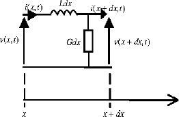
Figure 9.14. Elementary cell of the LG line
L and G are inductance and conductance densities.
Then
If dx → 0, we obtain
Similarly
Therefore, if dx → 0
Differentiation of [9.183] with respect to x leads to
This means that the equations of the LG line
are in fact the classical diffusive equations.
Using the Laplace transform and its differentiation properties, we obtain
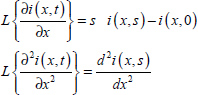
With the hypothesis i(x, 0) = 0, equation [9.187] becomes
Let us define
Then, the general solution of [9.190] is
For an infinite length line, we have
and finally
Then
Let us define the complex impedance of the LG line
thus
The complex impedance is equivalent to a fractional differentiator with n = 0.5, regardless of x.
Thus
and
or equivalently
This equation defines the fractional inductor with
A.9.2. Energy storage and dissipation in the fractional capacitor
The fractional capacitor C* is characterized by the equation
A distributed model is associated with this equation
Our objective is to express the stored energy E(t) and its dissipation P(t) with the analog distributed network {R(ω), C(ω)} (see Chapter 7).
The input of this network is the current i(t), and its output is the voltage v(t).
Equation [9.203] gives
Moreover, for the elementary cell {R(ω), C(ω)}, we can write
Finally, the total voltage v(t) is expressed as
therefore we obtain
This equality is verified with the constraints
Thus, we can express the stored energy
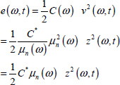
i.e.
For the dissipation of energy, we obtain
thus
i.e.
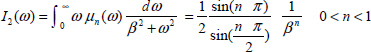
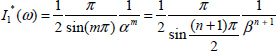
A.9.3. Some integrals
Consider the distributed model of the fractional integrator. If the input is a Dirac impulse v(t) = δ(t), then z(ω, t) = e–ωt and
With ![]()
The Laplace transform of [9.214] provides
if s is real, such as s = β, then
and
Let us define
Consider the new variables ω2 = u β2 = α, so ![]() and
and ![]() .
.
Then
Define ![]() .
.
Therefore
and
Thus
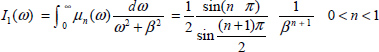
Define
Using the previous variables u and α, we obtain
Consequently