
1
Initialization of Fractional Order Systems
1.1. Introduction
The initialization problem, or the initial value problem, is considered an elementary topic in the integer order case. On the contrary, for a long time it has been considered a very complex problem in the fractional order case; certainly because fractional derivatives, mainly Caputo’s derivative, have perpetuated a deep confusion about initial conditions (see Chapter 8 of Volume 1).
The initialization of an ODE is an obvious problem. Initial conditions are well defined because this concept directly refers (or indirectly) to the system state ![]() [KAI 80, CHE 84, ZAD 08]. In the fractional order case, the definition of system state has been confused for a long time because it was not possible to directly generalize the concepts of integer order state space to fractional systems. As demonstrated previously, the variable x(t), output of the fractional order integrator, is only a pseudo-state variable, unable to represent the true internal state of the fractional system (see Chapter 7 of Volume 1). Moreover, since the so-called initial conditions of Caputo’s derivative were considered as the value of the system state at t =0, it was impossible to predict the future system dynamics based on these pseudo-initial conditions, as in the integer order case (see Chapter 8 of Volume 1). Thus, the initialization of fractional systems seemed an inextricable problem. There are many publications related to the initialization of fractional systems; the reader can refer to [FUK 03, ORT 03, FUK 04, ORT 08, SAB 10a] and to the overview [TEN 14].
[KAI 80, CHE 84, ZAD 08]. In the fractional order case, the definition of system state has been confused for a long time because it was not possible to directly generalize the concepts of integer order state space to fractional systems. As demonstrated previously, the variable x(t), output of the fractional order integrator, is only a pseudo-state variable, unable to represent the true internal state of the fractional system (see Chapter 7 of Volume 1). Moreover, since the so-called initial conditions of Caputo’s derivative were considered as the value of the system state at t =0, it was impossible to predict the future system dynamics based on these pseudo-initial conditions, as in the integer order case (see Chapter 8 of Volume 1). Thus, the initialization of fractional systems seemed an inextricable problem. There are many publications related to the initialization of fractional systems; the reader can refer to [FUK 03, ORT 03, FUK 04, ORT 08, SAB 10a] and to the overview [TEN 14].
However, Lorenzo and Hartley, aware of these difficulties, proposed a methodology to avoid explicit reference to the system state [LOR 01, HAR 02, LOR 08a, LOR 08b, GAM 11]. This technique, known as the history function approach [HAR 09b, HAR 11], can be considered as an input/output method, independent of the true internal system state. More recently, the infinite state approach has given a solution to the initialization problem in terms of the system state [TRI 09b, TRI 11a, TRI 11d, TRI 12a, TRI 12b, TRI 12c, TAR 16a, TAR 16c]. As stated previously, the pseudo state x(t) is replaced by z(ω, t), which is the internal distributed state of any fractional order system; therefore, initialization can be treated as in the integer order case. Moreover, a collaboration between the two research teams exhibited the equivalence and the complementarity of the two approaches [HAR 13], which will be mentioned later. Some papers rely on these two approaches [DU 11, MAO 15, YUA 18, ZHA 18]. However, practical initialization remains a difficult problem.
Despite the attractiveness of the history function approach, it only provides tractable solutions in a limited number of theoretical cases [HAR 11]. Similarly, although the infinite state approach makes it possible to use the same techniques as in the integer order case, such as state observers [TRI 11a], accurate estimation of the initial state remains a difficult topic, mainly caused by the infinite dimension of this state. Therefore, this section is only dedicated to the fundamentals of initialization; a practical solution will be proposed in Chapter 3. In fact, as demonstrated in Chapters 6, 7 and 8 of Volume 1, theoretical fractional system initialization can be considered as a solved problem. However, a comparative analysis of the two approaches is useful to extract the fundamentals of initialization of fractional systems.
1.2. Initialization of an integer order differential system
1.2.1. Introduction
There are two distinct problems: the initial values of an ordinary differential equation (known as the initial value problem) [KOR 68] and the response of this ODE to any excitation u(t) that takes into account initial conditions at t = t0, summarizing the past behavior of the system. As the solution of the first problem is straightforward, only the second problem will be discussed.
1.2.2. Response of a linear system
Consider the linear system characterized by the transfer function H(s) = L{h(t)} (where h(t) is the impulse response) with input u(t) and output y(t). The model H(s) corresponds to an input/output representation, i.e.
A state space model can be associated with this system
where ![]() is the system state.
is the system state.
Assume that we consider the behavior of this system since t = –a (the system is assumed to be initially at rest at t = –a).
The objective is to express the system response y(t) for t ≥ 0 without the explicit use of past behavior, corresponding to –a < t < 0.
According to the linear system theory, y(t) must take into account this past behavior using initial conditions ![]() at t = 0, thanks to a free response or an initialization function ψ(t), and a forced response caused by the excitation u(t) for t > 0 [KAI 80]; therefore
at t = 0, thanks to a free response or an initialization function ψ(t), and a forced response caused by the excitation u(t) for t > 0 [KAI 80]; therefore
This problem can be summarized by the graphs presented in Figure 1.1.
Let us call history functions (or past behavior, or pre-history) the graphs of u(t) and y(t) for –a < t < 0.
Usually, the solution y(t) (t > 0) is expressed using a state space representation, with the explicit use of ![]() .
.
However, it is also possible to express y(t) with a convolution integral (i.e. with an input/output approach), without the explicit use of the initial state ![]() . This second solution is used by Lorenzo and Hartley in the history function approach, whereas the infinite state approach refers to a state space representation, i.e. to the first solution.
. This second solution is used by Lorenzo and Hartley in the history function approach, whereas the infinite state approach refers to a state space representation, i.e. to the first solution.

Figure 1.1. The initialization problem
1.2.3. Input/output solution
Let us express the convolution y(t) = h(t)*u(t) since t = –a :
y(t) can be expressed as the sum of two integrals, from τ = –a to 0 and from τ = 0 to t.
Therefore
Then, let us define
and
1.2.4. State space solution
Let ![]() be the system state at t = 0, summarizing the past behavior from τ = –a to τ = 0.
be the system state at t = 0, summarizing the past behavior from τ = –a to τ = 0.
Then, on the one hand
and on the other hand

REMARK 1.– The input/output solution, expressed with the impulse response, refers only to the observable and controllable part of the system state [KAI 80, ZAD 08]. On the contrary, the state space solution takes into account all state components; therefore, it represents the more complete solution.
REMARK 2.– As ![]() for t ≤ –a, we can write
for t ≤ –a, we can write

Therefore
Using [1.10], we obtain
i.e.
Thus, we can verify the fundamental equality
1.2.5. First-order system example
Consider the first-order system
and its impulse response
Let us apply a step input U at instant t = –a.
Therefore
Then (see Figure 1.2)

Figure 1.2. Step response of a first-order system
Obviously
Then, the free response is expressed as
We can also write
i.e.
Thus, we verify again that the input/output and the state space representations are equivalent:
1.3. Initialization of a fractional differential equation
1.3.1. Introduction
As mentioned in the introduction, the initialization of an FDE cannot be performed as in the integer order case, using the initial value of the pseudo-state variable ![]() . It has been proved that the knowledge of
. It has been proved that the knowledge of ![]() is unable to give information on the future behavior of the FDE (see Chapters 7 and 8 of Volume 1). In fact, the future behavior depends on the initial value of the internal distributed state variables zi(ω, 0), with
is unable to give information on the future behavior of the FDE (see Chapters 7 and 8 of Volume 1). In fact, the future behavior depends on the initial value of the internal distributed state variables zi(ω, 0), with
Let us remember that an infinity of different dynamics (each one depending on a particular frequency distribution zi(ω, 0)) can correspond to the same pseudo-initial value xi(0) [TAR 16a, TAR 16c]. As the general problem was treated previously (see Chapter 7 of Volume 1), we only present thereafter some simulation examples for a one-derivative FDE, in order to illustrate the dependence of dynamics on the initial distributed state z(ω, 0).
1.3.2. Free response of a simple FDE
Consider the elementary FDE
The following distributed differential system is associated with this FDE:

The distributed initial condition is z(ω, 0), which verifies the initial value
In order to emphasize the dependence of x(t) (t > 0) on z(ω, 0), we consider a numerical simulation of [1.25, 1.26] with three different distributions z(ω, 0) corresponding to the same value x(0) [1.27].
Therefore, system [1.25] is frequency discretized (see Chapter 2 of Volume 1):

The simulation parameters are
Each initial condition z(ω, 0) corresponds to the discretized distribution
with the constraint
Three distributions are considered: they are designed to correspond to the same initial value x(0):
1) zj(0) = 0 for j = 1 to J, with
2) ![]() with
with
3) ![]() with
with
The distribution [1.32] corresponds to the pseudo-initial condition of Caputo, requiring x(t) = cte = x(0) for t = –∞ to 0 (see Chapter 3 of Volume 1).
Therefore, x(0) depends only on z0 (0) (zj(0) = 0). It corresponds to the slower decrease of x(t), as observed in Figure 1.3.
Distributions [1.33] and [1.34] have components at high frequency. Their amplitude decrease with frequency; however, the high-frequency components of distribution [1.33] are relatively more important than those of distribution [1.34] (see Figure 1.4). Consequently, the decrease of x(t) with distribution [1.33] is faster than with distribution [1.34] (see Figure 1.3).
Although the considered distributions are essentially theoretical, the main conclusion is that the corresponding transients characterized by the same initial value x(0) are completely different. Obviously, the knowledge of x(0) is of no help to explain the different dynamics of x(t), because these dynamics depend essentially on z(ω, 0).

Figure 1.3. Free responses with the same initial value. For a color version of the figures in this chapter see www.iste.co.uk/trigeassou/analysis2.zip
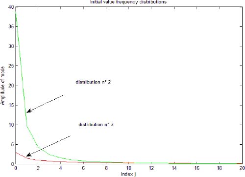
Figure 1.4. Comparison of distributions 2 and 3
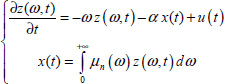
1.4. Initialization of a fractional differential system
1.4.1. Introduction
The initialization of an FDS is closely related to the initialization of its integer order counterpart (see section 1.2). There are two approaches: one deals with the input/output formulation, and the other deals with the state space representation. However, the analysis of this problem is more complex, mainly caused by the duality between the pseudo-state variables and the distributed internal state variables. Moreover, in contrast with the integer order case, analytical solutions can be formulated only in a limited number of particular cases.
The principles of the two approaches are presented later in a theoretical framework. Some examples are used to illustrate these two methodologies in the next section.
1.4.2. State space representation
The presentation is limited to the case of an N-derivative commensurate order FDS.
Consider
A distributed integer order differential system is associated with [1.35]:

Let Ẕ(ω, 0) be the distributed initial state at t = 0.
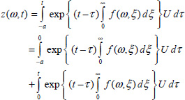
As demonstrated in Chapter 9 of Volume 1, the general response of [1.35, 1.36] to the excitation u(t) with the initial state Ẕ(ω, 0) can be expressed using
the Mittag-Leffler technique as
where
![]() represents the free responses of the N integrators
represents the free responses of the N integrators ![]() associated with [1.35, 1.36]. ũ(t) is an equivalent input [MON 10] expressed as
associated with [1.35, 1.36]. ũ(t) is an equivalent input [MON 10] expressed as
En,1 (Atn) is the matrix Mittag-Leffler function.
The first term of [1.37] represents the free response or the initialization function of the pseudo-state ![]() .
.
Thus, the initialization function of y(t) is expressed as
Obviously, it will be very difficult to analytically express ψ(t) in the general case.
1.4.3. Input/output formulation
Let Hn(s) be the transfer function of [1.35]:
Let hn(t) be its impulse response:
Therefore, we can write
As noted previously, the convolution integral is calculated since t = –a, and the system is assumed to be at rest for t < –a.
Therefore
which corresponds to
Thus, the general expression of the initialization function is
and the forced response is expressed as
The history function approach of Lorenzo and Hartley corresponds to the application of this input/output methodology [LOR 01, HAR 11].
The authors’ main objective was to express ψ(t) using the Mittag-Leffler function and the incomplete Gamma function [HAR 07].
Moreover, they were forced to use simplifying assumptions, such as constant and ramp history functions, in order to formulate analytical expressions of ψ(t) [HAR 09b, HAR 09c].
1.5. Some initialization examples
1.5.1. Introduction
A comparative analysis of the two approaches was published in [HAR 13]. Two simple examples were used: initialization of the fractional integrator and the fractional differentiator.
They are presented later. A third example that deals with an elementary FDS is also presented to illustrate the complexity of analytical fractional order initialization.
1.5.2. Initialization of the fractional integrator
Consider the elementary integrator
excited by a Dirac impulse at instant t = –a.
Therefore
and
1.5.2.1. State space approach
Let z(ω,t) be the distributed variable of ![]() defined by:
defined by:
Thus, at instant t = 0, we obtain
Hence, for t > 0
and
As (Appendix A.1. Chapter 1 Volume 1)
we obtain
1.5.2.2. Input/output approach
Recall that
Then
Let
Therefore, we obtain [HAR 13]
where Γ(n, as) is the incomplete gamma function [HAR 07].
As
We finally obtain
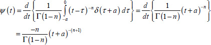
REMARK 3.– We can directly obtain ψ(t) without using its Laplace transform ψ(s).
Since
Using [1.59], we directly obtain
1.5.3. Initialization of the Riemann-Liouville derivative
The Riemann-Liouville derivative is defined by the relation
As stated previously, we apply a Dirac impulse at t = –a, i.e. u(t) = δ(t + a).
1.5.3.1. State space approach
Let zRL(ω, t) be the distributed variable associated with ![]() :
:
Therefore
Then, for t > 0
Therefore
As
we obtain
thus
1.5.3.2. Input/output approach
Let us define α = 1 – n and q = n; Lorenzo and Hartley demonstrate [HAR 13] that
Thus
REMARK 4.– Again, we can directly express ψ(t) without the Laplace transform ψ(s).
Using the definition of x(t)
Then
1.5.4. Initialization of an elementary FDS
1.5.4.1. Introduction
Consider the initialization of the elementary FDS at t = 0:
excited by a step input U at t = –a, so u(t) = UH(t + a); this system is assumed to be at rest at t = –a.
This example is used to illustrate the complexity of the initialization problem for a system less basic than the integrator or the differentiator.
Two fractional system representations will be used: the closed-loop formulation and the open-loop formulation (see Chapter 7 of Volume 1).
1.5.4.2. Open-loop model formulation
Consider again
Using the inverse Laplace transform, we can express its impulse response hn(t) as
with (see Chapter 7 of Volume 1)
The open-loop model is characterized by the distributed variable ξ(ω, t):
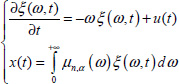
where
Our objective is to initialize this system at t = 0 using ξ(ω, t) and ξ(ω, 0).
1) State space approach
Then
and
Therefore
and
2) Input/output approach
x(t) is defined as
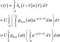
Therefore

Obviously, equation [1.88] exactly corresponds to [1.86].
1.5.4.3. Closed-loop model, Mittag-Leffler formulation
The system [1.78] corresponds to the elementary FDS:
and to the closed-loop distributed model (recall that ξ(ω, t) ≠ z(ω, t)):
1) Input/output approach
Let us recall that if u(t) = UH(t) or ![]() , we can express
, we can express
As (see Chapter 3 of Volume 1)
we can write
As
we obtain
If we use a step input applied at t = –a, it is necessary to translate the time scale; thus
This result corresponds to
and
Note that if we use the fictive excitation ũ(t)
we can write
therefore
Using [1.99], we obtain the expression of ψ(t)
i.e. for t > 0
We can conclude that the history function approach (input/output approach) provides an analytic formulation of the initialization function ψ(t).
2) State space approach
With u(t) = UH(t) and no initial condition, the Laplace transform of [1.90] gives

As
we obtain
Therefore, as [1.94]
we obtain
For u(t) = UH(t + a) (i.e. a step input at t = –a), we can write
If we want to initialize the system at t = 0, we obtain
Thus, the free response of [1.89] for t ≥ 0, using z(ω, 0), is expressed as
where x0(t) is the free response of ![]() :
:
Therefore
An expression of ψ(t) can be formulated as
where
Obviously, it will be difficult to obtain an analytical formulation of ψ(t) in order to compare it to [1.103].
However, we can verify the identity of equations [1.103] and [1.113] that perform a numerical simulation.
Therefore, we use the frequency discretized model of [1.90], i.e.

The following simulation parameters are used:
J = 20; ωb = 10–3 rd/s; ωh = 10+3 rd/s; Te = 10–3 s; a = 2.5s; U = 1; α = 1
The simulation of [1.115] provides z(ω, 0) at t = 0.
Then, the initialization function ψ(t) is provided by the distributed model [1.90] initialized by z(ω, 0) with u(t) = 0:


Figure 1.5. Comparison of initialization functions
Figure 1.5 presents x(t) provided by equation [1.115], ψ(t) provided by [1.116] and ψ(t) provided by [1.103].
Thus, we numerically verify that the two expressions of ψ(t) are identical.
1.5.4.4. Closed-loop model and distributed exponential formulation
In Chapter 9 of Volume 1, we expressed FDS transients using two approaches: the Mittag-Leffler technique and the distributed exponential formulation. Thus, we intend to express ψ(t) with this new formulation, in order to highlight its potentialities.
Consider again the elementary FDS [1.89]:
corresponding to the distributed differential system [1.90].
The step response of the distributed state z(ω, t) with z(ω, –a) = 0 ∀ ω and u(t) = UH(t + a) is expressed as
Therefore, we can define
where
is the distributed exponential with
(see the definitions of Chapter 9 of Volume 1).
Finally
1) State space formulation
Let us define
We can express

Therefore
Note that
Thus
and
REMARK 5.– If n = 1, then μ1(ω) = δ(ω); therefore, f(ω, ξ) = –αδ(ω).
Then,![]() and exp{t g(0, α)} = e–αt.
and exp{t g(0, α)} = e–αt.
Therefore, ![]()
and ![]()
This result corresponds of course to [1.22].
2) Input/output formulation
As mentioned previously, using the fictive input ũ(t) [1.99]
we can write
where
and
since z(ω, 0) = 1 ∀ ω when system [1.89] is excited by a Dirac impulse δ(t).
Then

therefore
Since
we obtain
i.e. the same result [1.127] as obtained previously.
REMARK 6.– Using the Mittag-Leffler formulation:
therefore
If n =1, the right side of [1.138] is equal to
REMARK 7.– Using the distributed exponential formulation, we obtain results that are equivalent to those of the integer order case (section 1.2.5).
This means that this formulation makes it possible to generalize the integer order case: this is obviously interesting to derive mathematical proofs. However, we have to keep in mind that the apparent simplicity of the distributed exponential formulation hides, in fact, major computational complexity (see Chapter 9 of Volume 1).
1.5.5. Conclusion
The previous comparative analysis has made it possible to formally verify the equivalence of the history function and infinite state approaches, each of which provides a solution to the initialization of linear fractional differential systems. However, these theoretical approaches cannot provide an analytical solution for systems more complex than the one-derivative FDS.
Moreover, the theoretical assumptions of this comparative analysis are too restrictive, particularly the assumption that the system is at rest at instant t = –a is not realistic.
In fact, this analysis has proved the influence of past behavior on initialization (or long memory phenomenon). Theoretically, we have to take into account all the dynamical history of the system, since t = –∞.
Practically, it will be necessary to truncate past dynamical behavior (or pre-history). Therefore, the system cannot be considered at rest at instant t = –a.
Thus, the practical initialization based on an arbitrary truncated dynamical past behavior is studied in Chapter 3.