
Propensity Score Stratification and Regression
2.2 Propensity Score: Definition and Rationale
2.3 Estimation of Propensity Scores
2.4 Using Propensity Scores to Estimate Treatment Effects: Stratification and Regression Adjustment
2.5 Evaluation of Propensity Scores
2.6 Limitations and Advantages of Propensity Scores
Comparing the effectiveness of interventions in nonrandomized studies is difficult because usually there are baseline differences between the interventions. Propensity scores are a suitable methodology for adjusting for such differences and, therefore, for obtaining unbiased effectiveness estimates. In this chapter, stratification and regression methods, two commonly used propensity score approaches, are presented. To illustrate, data from an observational study comparing the effectiveness of two antidepressant treatments were analyzed by using stratification and regression propensity score methods.
One of the main aims of medical studies is to elucidate causality between medical interventions or treatments and health outcomes. Randomized clinical trials (RCTs) are the gold standard study designs for judging treatment benefits (Grimes and Schulz, 2002). However, the controlled circumstances in which they are conducted limit the generalizability of results to day-to-day clinical practice (Rothwell, 2005). Furthermore, there are situations in which they are not feasible for either ethical or practical reasons. Observational studies are considered to complement RCTs because they aim to represent the real clinical situation (McKee et al., 1999). Their design maximizes external validity, but this is usually at the expense of losing some degree of internal validity.
In RCTs, treatment influences on outcomes are usually considered as causal because the patients taking different treatments are supposed to be exchangeable (i.e., their characteristics, except the intervention that is evaluated, are expected to be the same) (Hernán, 2004). However, in observational studies, the assumption of exchangeability is not valid because patients are prescribed different medications precisely because they differ in prognostic factors (Hernán and Robins, 2006a). Hence, applying sound statistical methods to reduce confounding is needed when analyzing observational studies.
2.2 Propensity Score: Definition and Rationale
In 1983, Rosenbaum and Rubin developed the concept of propensity scores as an alternative to conventional multivariable regression modeling to estimate the effects of interventions or treatments in observational studies. The goal of propensity scores is to balance observed covariates between subjects from the study groups (usually two groups: treatment and control) in order to mimic what happens in a randomized study (Joffe and Rosenbaum, 1999).
To formally define the concept of propensity score, we need some notation. Let X represent the observed covariates for the subjects included in the study (observed before treatment is assigned) and Z represent an indicator of subject treatment (i.e., Z=1 if treated and Z=0 if control). Then, the propensity score for a subject is the conditional probability of exposure to treatment given his/her observed covariates, or PS=P[Z=1|X].
The propensity score has several theoretical properties that have been rigorously proven elsewhere (Rosenbaum and Rubin, 1983) and, therefore, they are not shown here. Nevertheless, insight into how propensity scores achieve balance is presented. In a balanced two-arm randomized study, the propensity score of each patient is equal to 1/2 for every X (i.e., subjects with different observed covariates have the same probability of receiving treatment, and reversibly each possible value of the observed covariates is as likely to occur in either of the two groups). Typically, in observational studies there are subjects that are more likely to receive treatment than to be controls because of some of the pre-treatment characteristics included in the observed covariates X, i.e., PS=P[Z=1|X]>1/2. Analogously, other subjects are more likely to be controls than to receive treatment given X, i.e., PS<1/2. However, suppose that we compare two subjects who have the same propensity score (for instance PS=1/3 for both subjects). These subjects could be different in terms of their observed covariate X’s. What is important is that these differences cannot predict which subject has more chance of receiving treatment. Given their observed covariates, both have the same probability (1/3) to be treated despite being quite different in terms of X’s. Hence, if we group subjects with the same propensity scores, both treated and control subjects in these groups will have on average covariate patterns similar to those that would occur in a randomized study.
2.3 Estimation of Propensity Scores
Generally, propensity scores are unknown in observational studies and, therefore, they must be estimated from data. Several methods are available (Setoguchi et al., 2008; Woo et al., 2008):
• probit regression
• discriminant analysis
• classification and regression trees
• neural networks
• generalized additive models
However, they are most commonly estimated by logistic regression. The dependent variable of the logistic regression is Z, with Z=1 the event of being in the treated group, and the independent variables are the observed covariates X. These variables can be both categorical or continuous.
Despite the common use of propensity scoring, there is little guidance on the details of building the propensity score model (i.e., which variables should be included in the model). Weitzen and colleagues (2004) surveyed the methods utilized in the literature and found a variety of approaches—including the non-parsimonious approach, univariate significance testing, various stepwise approaches, a priori selection, and goodness-of-fit testing. Further research (Weitzen et al., 2005) led them not to recommend goodness-of-fit testing. However, no single method was demonstrated as clearly superior. Common advice is to err toward being overinclusive in order to avoid leaving out a confounding variable. That is, add all covariates potentially related to outcome and exposure (even if the p-value is greater than 0.05) and consider nonlinear terms for continuous measures. This is recommended because only the predicted values are utilized, not the parameter estimates for the model factors, so modeling issues such as overparameterization and collinearity are not considered critical here.
Brookhardt and colleagues (2006) as well as Senn and colleagues (2007) pointed out that a non-parsimonious approach of including all possible covariates is not without its disadvantages. They argue that including variables that are related to treatment selection but not outcome, or including variables not related to outcome, decreases the efficiency of the analysis. Thus, optimal selection of a model is likely not one where all variables are included.
While there is not complete consensus in the literature on the best method for modeling the propensity score, there is general agreement that the most important issue is that the propensity score produces balance between the groups (Weitzen et al., 2004; D’Agostino, 1998). In fact D’Agostino and D’Agostino (2007) state that “the success of the propensity score modelling is judged by whether balance on pretreatment characteristics is achieved between the treatment and control groups.”
In practice, we have often utilized prespecification of covariates followed by a thorough sensitivity analysis. In this chapter, we focus not on modeling but on methods to assess the balance achieved by the propensity adjustment on the treatment groups (see Section 2.5).
To aid the credibility of the analysis, Rubin (2007) recommends completing the estimation of the propensity score prior to accessing the outcome data. Thus, one can guarantee that the choice of the propensity model is not influenced by its impact on the final analysis. That is, one did not run multiple analyses with various propensity models, and choose the model that ultimately produced the most desired results for the researcher. This approach to completing the propensity score modeling by no means eliminates the need for thorough sensitivity analyses, but it appears to us to be a useful approach, especially for prospective observational research.
Also note that if more than two treatments are compared, propensity scores for each treatment can be estimated by fitting a multinomial logistic regression, selecting one treatment as the reference category (Imbens, 2000).
2.4 Using Propensity Scores to Estimate Treatment Effects: Stratification and Regression Adjustment
Once the propensity scores are estimated, there are several ways they can be used to control for confounding. These include stratification, regression adjustment as a covariate into a multivariable regression model, and matching, among others (Austin and Mamdani, 2006; D’Agostino, 1998; Rosenbaum and Rubin, 1983). In this chapter, we focus on the two first methods. Propensity score matching is covered in Chapter 3.
In propensity score stratification, subjects are stratified into groups based on their estimated propensity scores. The use of five groups, based on quintiles of the propensity score, is common because it was shown that five groups can remove approximately 90% of the bias from a confounding variable (Cochran, 1968). However, when sample sizes are large, such as in the analysis of health care claims databases, the use of a larger number of propensity score groups produces greater homogeneity among patients within groups. Of course, too many propensity groups may result in small or zero sample sizes for particular treatments within propensity groups. While there is no clear guideline on the optimal number of propensity groups, one should consider these tradeoffs and thorough analyses to make sure that results are insensitive to rationale choices on the number of propensity groups.
Once the patients have been grouped into homogeneous strata based on their propensity scores, treatment differences are estimated within each quintile, and the five estimated treatment effects are pooled into one overall treatment effect. The basic idea is, as in stratification, valid comparisons are made as treatments are compared within like patients—with like being defined as patients with similar propensity scores.
In propensity score regression adjustment, the treatment effect is estimated by a multivariable regression model that includes as covariates an indicator of treatment, Z, and the propensity score itself, either as a continuous covariate or as a categorical covariate by using the propensity score quintile as a categorical variable. For more than two treatments, the propensity scores of all treatments except the propensity scores of the reference treatment must be included as covariates into the multivariable regression model either as continuous covariates or as categorical covariates by using the propensity score quintiles as categories.
While there is a lack of detailed guidance from theoretical or simulation research in this area, often researchers include additional variables in the multivariable regression model (D’Agostino and D’Agostino, 2007; Cadarette et al., 2008). D’Agostino and D’Agostino (2007) suggest fitting a model to estimate the treatment effect that includes a subset of patient characteristics that are thought to be the most important known potential confounders. This is done in order to add precision to the treatment effect estimate (as one would do in a regression model analysis of a randomized trial) and adjust for any residual imbalances that might exist after the propensity score modeling. Thus, either variables with strong relationship with the outcome measure or variables with noted residual imbalance after propensity scoring might be included. A similar extension for the propensity score stratification analysis is to utilize a regression model for each quintile stratum analyses. Such extensions correspond to the doubly robust approaches presented in Chapter 4 (see also Lunceford and Davidian, 2004).
Regardless of whether propensity score stratification or propensity score regression is selected, a thorough evaluation of the success of the propensity adjustment should be made prior to performing the outcome analysis. The primary function of the propensity scoring is to account for confounding. Thus, as discussed in Section 2.3, the use of the propensity scores should produce balance across covariates between the treatments being compared. Specific methods for assessing the balance produced by propensity adjustment are described in Section 2.5.
Last, sensitivity analyses are critical. Producing causal inferences from observational data requires assumptions beyond those in randomized research (e.g., no unmeasured confounders, positivity), and such assumptions should be examined. For instance, while one cannot ever prove there are no missing confounders, one can consider running an analysis that may relax this assumption, such as an instrumental variable analysis (as described in Chapter 6). However, to obtain unbiased estimates with an instrumental variable, several other strong conditions must hold (Hernán and Robins, 2006b). Another option is quantifying the sensitivity of the results to unmeasured confounding (Schneeweiss, 2006; see also Section 2.6.1). Examination of the propensity distribution for each treatment group can aid in assessing positivity (positive probability for selection of each treatment for any combination of covariates). Sensitivity surrounding the covariate balance within treatment groups can be assessed by using methods such as propensity score matching, which can provide superior balance but with the potential tradeoff of a reduced sample (Austin et al., 2007a).
In summary, a quality propensity score stratification or regression analysis involves more than simply estimating the propensity score and running an adjusted model. Quality analyses include an assessment of the balance produced by the propensity score, assessment of statistical assumptions, sensitivity analyses, and transparency in reporting. Transparency is important as a reader should be able to understand the quality of the analyses that were performed, knowing what decisions were made, when they were made, and why.
2.5 Evaluation of Propensity Scores
In the report of a randomized study, a table comparing the distribution of the most important pretreatment assignment covariates between treatment and control groups is usually shown in order to assess if randomization was effective. Because the objective of propensity scores is to create a quasi-randomized experiment from a non-randomized observational study, a similar approach can be performed to assess if the quasi-randomization was achieved. As discussed in Section 2.3, the key assessment of the success of the propensity score adjustment is demonstrating that the propensity score produced balance between the treatments for comparisons.
There are multiple approaches to assessing the balance produced by a propensity model. Austin and Mamdani (2006) and Austin (2008) provide a nice summary of methods. At a high level the methods include the following:
1. assessment of standardized differences of each covariate between treatment groups
2. assessment of the propensity score distribution
3. comparison of distributions of the covariates between treatments
4. assessment of goodness-of-fit statistics
More specifically, for propensity score stratification analyses, because the treatment comparisons are ultimately made within each propensity score stratum, the focus is on assessing balance within strata. Three common approaches for propensity score stratification balance assessment are the use of two-way ANOVA modeling for each covariate, within-strata standardized differences for each covariate, and within-strata side-by-side box plots of the propensity score and covariate distributions.
Rosenbaum and Rubin (1984) proposed a two-way ANOVA (or logistic regression for binary covariates), with each covariate as the dependent variable and a model including treatment, propensity score strata, and the interaction of treatment and propensity score strata. This approach detects differences in mean covariate values between the treatment groups that are both consistent across strata (significance of the treatment factor) and not consistent (significance of the interaction term). This approach corresponds to standard baseline comparison tables commonly used in randomized controlled trials and is thus readily accepted.
Standardized differences are defined here as the difference in means between the two groups divided by a measure of the standard deviation of the variable. Standardized differences can be computed for both continuous and binary covariates (Austin, 2008). Computation of the standardized differences for all covariates allows for an assessment, on a common scale, of differences in means between treatment groups within each quintile. One can then identify the specific covariates with the largest residual imbalance after propensity adjustment. As a rule of thumb, standardized differences greater than 0.10 indicate an imbalance that might require further investigation (Austin and Mamdani, 2006).
As opposed to standardized differences, which assess differences in means, box plots can be used to investigate differences in the distributions of a covariate or the propensity score between the treatment groups. If balancing is achieved, one would expect that the distributions of propensity scores for treated and control groups within each quintile are similar (Austin and Mamdani, 2006). Also, by investigating the overall distribution of the propensity scores, one can detect if there are different ranges for the two treatment groups that might indicate a violation of the positivity assumption. Recall that positivity (positive probability for either treatment group being selected regardless of the combination of the covariates) is a key assumption for causal inference. If box plots identify nonoverlapping regions (i.e., patients in one group have propensity scores in a given range but patients in the other group do not), this should result in further investigation by the researcher. For instance, sensitivity analyses without patients in nonoverlapping regions should be conducted.
As mentioned previously, these balance diagnostics may suggest the need for modification of the propensity model or other sensitivity analyses. For instance, one can modify the propensity model by adding or deleting covariates, adding interaction terms, or adding nonlinear terms for the continuous covariates.
For propensity score regression analyses, fewer methods have been developed for assessing balance. The assumption for analysis here is that patients in both treatment groups who have the same propensity score will have similar distributions of the covariates. Two approaches have been proposed for propensity regression analyses: weighted conditional standardized differences and quantile regression. The standardized differences approach corresponds to assessments for propensity stratification and matching analyses. Standardized differences are estimated at each value of the propensity score and averaged across the observed distribution of propensity scores. Quantile regression assesses the distribution of the covariates for patients in each treatment group with the same propensity score. We demonstrate here the assessment of the weighted standardized differences—given its similarity to methods used for other propensity based analyses. We also recommend assessing the distribution of propensity scores in this situation as well—to avoid positivity assumption violations. In addition, when propensity score regression is used with propensity score strata as the covariate, the methods for assessing balance in the stratification analysis could be utilized.
2.6 Limitations and Advantages of Propensity Scores
2.6.1 Unmeasured Confounding
The main limitation of propensity scores is that they do not control for unobserved covariates (or hidden bias) unless they are correlated with the observed covariates X’s (Haro et al., 2006). However, this is a limitation of observational studies rather than a limitation of the technique itself. The usual way to avoid hidden bias is by designing a randomized experiment but, as we have discussed previously, a randomized study may be not feasible or it may have low external validity. Nevertheless, Rosenbaum (2002) has proposed sensitivity analyses that indicate the magnitude of hidden bias that would need to be present to modify the conclusion of an observational study. Schneeweiss (2006) provides an overview of various approaches to assessing the sensitivity of observed results to potential unmeasured confounding. These approaches include quantifying the level of unmeasured confounding necessary to change the observed results (e.g., the rule out approach) and internal or external adjustment. StÜrmer and colleagues (2005) provide an example of internal adjustment, specifically propensity score calibration. This approach is possible when detailed information on a subset of patients is available to make the propensity adjustment computed based on a limited number of variables in the full set of patients. McCandless and colleagues (2007) also provide a Bayesian approach to such sensitivity analyses.
2.6.2 Propensity Score vs Conventional Regression
The use of conventional regression modeling, where potential confounders are simply entered directly into the regression model as opposed to the use of a propensity score, is common in observational research. In fact, in a survey of the literature, Shah and colleagues (2005) noted that among 78 comparisons where both conventional regression and propensity scoring were used, there was disagreement in the results in only 10% of the cases. In each case of disagreement, the propensity approach produced more conservative results. StÜrmer and colleagues (2006), in another review of the published literature through 2003, found agreement between conventional regression and propensity score approaches in nearly 90% of the reports. While in many cases similar results can be obtained, there are important potential advantages to a propensity based approach.
To begin, since the goal of the first step of the propensity score process is to obtain the best estimated probabilities of treatment assignment, one is not concerned with overparameterization of the model and, therefore, can include, for example, nonlinear terms or interactions. Then, once the propensity scores are estimated, one can include only treatment, propensity scores, and a small subset of the most important observed covariates into the final model. In this simple model, diagnostic checks can be performed more easily than in a more complex multivariable regression model that includes more variables (D’Agostino, 1998).
Second, if we are studying a rare dichotomous health outcome but the treatment is common, propensity scores may be a better option than conventional logistic regression. In this case, adjustment using propensity scoring is feasible; however, the conventional logistic regression may not be if we need to include many confounding covariates into the model (Braitman and Rosenbaum, 2002). Moreover, it has been proven by Monte Carlo simulations that if we have less than eight events per confounder, propensity score estimates are a better alternative than logistic regression to control for imbalances (Cepeda et al., 2003).
In addition, a simulation study suggests that regression is more efficient than propensity scoring when the model is correctly specified, but propensity score estimates are much more robust to model misspecification than classical multivariable regressions (Lunceford and Davidian, 2004). Thus, propensity scoring is recommended because situations where we know the model is completely correct are limited to simulation studies. Another simulation study shows that propensity score methods, in general, give treatment effect estimates that are closer to the true treatment effect than a logistic regression model in which all confounders are modeled (Martens et al., 2008).
Others have noted various advantages of propensity scoring. Shah and colleagues (2005) noted that regression analysis does not alert investigators to situations where the confounders do not adequately overlap between treatment groups, threatening the validity of the conclusions. Such situations become obvious in a propensity score approach with the non-overlapping distributions. Thus, the ease in which regression can be conducted can falsely lead researchers to biased results. D’Agostino and D’Agostino (2007) noted that conventional regression can produce biased estimates of treatment effects if there is extreme imbalance of the background characteristics and/or the treatment effect is not constant across values of the background characteristics. Such scenarios are certainly possible in observational research.
Austin and colleagues (2007b) and Senn and colleagues (2007) noted there is also a fundamental difference between conventional regression, which obtains conditional estimates of the treatment effect, and propensity scoring, which estimates marginal treatment effects. Such approaches may differ in certain scenarios and readers are referred to these references for more details.
In summary, while in many situations the analyses will prove similar and either approach may be appropriate, propensity scoring is considered a more robust approach. One does not have to make additional assumptions regarding specific (e.g., linear) effects of the covariates on the outcome, and propensity analyses have built-in sensitivity checks.
2.7.1 Study Description
To illustrate the implementation of a propensity score analysis, we analyze simulated data based on a study of the effectiveness of medications for patients with depression in usual-care settings. A brief description of the study design follows. Data were simulated based on a study of 192 patients with depression who were treated with a new treatment A (experimental group) or with the usual treatment B (control group). The decision to treat patients with treatment A or B was based on the clinical judgment of physicians; hence, the treatment assignment was not randomized. Sociodemographic and clinical characteristics were recorded at the baseline visit: age, sex, marital status, employment, and symptom severity measured with the Patient Health Questionnaire (PHQ) score. The PHQ is a nine-item self-report questionnaire designed to evaluate the presence and severity of depressive symptoms. Each of the nine items can be scored from 0 to 3. Then, the final score can range from 0 (absence of depressive symptoms) to 27 (severe depressive symptoms). The outcome of interest for this analysis was remission at three months after the treatment initiation. Remission was defined as a score of 4 or less in the PHQ score at the three-month visit.
2.7.2 Data Analysis
Before conducting the propensity score analysis, we provide a brief summary of the data. The two treatment groups were balanced with respect to baseline patient characteristics except for baseline symptom severity: patients treated with B were more severe than patients treated with A (see Output 2.1 from Program 2.1). For simplicity of presentation, we considered only five covariates, though in practice one will likely encounter a longer list of potential confounders. After three months, the remission rate of patients treated with A was statistically significantly greater than patients treated with B (62.5% vs. 46.9%, p<0.05 using an unadjusted chi-square test).
Program 2.1 Baseline Group Comparisons
/* This section of code performs the baseline treatment */
/* comparisons */
PROC TTEST DATA=ADOS;
CLASS TX;
VAR AGE PHQ1;
RUN;
PROC FREQ DATA=ADOS;
TABLE (SEX SPOUSE WORK)*TX / CHISQ ;
RUN;
Output from Program 2.1
The TTEST Procedure
Statistics
| Lower CL | Upper CL | Lower CL | Upper | CL | |||||
| Variable | TX | N | Mean | Mean | Mean | Std Dev | Std Dev | Std Dev | Std Err |
| age | B | 96 | 42.329 | 45.344 | 48.359 | 13.033 | 14.881 | 17.345 | 1.5188 |
| age | A | 96 | 40.219 | 42.844 | 45.469 | 11.347 | 12.956 | 15.101 | 1.3223 |
| age | Diff | (1-2) | -1.472 | 2.5 | 6.4722 | 12.679 | 13.952 | 15.511 | 2.0138 |
| phql | B | 96 | 14.902 | 15.99 | 17.077 | 4.6991 | 5.3656 | 6.2541 | 0.5476 |
| phql | A | 96 | 12.568 | 13.688 | 14.807 | 4.8393 | 5.5257 | 6.4407 | 0.564 |
| Phql | Diff | (1-2) | 0.7515 | 2.3021 | 3.8527 | 4.9493 | 5.4462 | 6.0549 | 0.7861 |
T-Tests
| Variable | Method | Variances | DF | t Value | Pr > |t| |
| age | Pooled | Equal | 190 | 1.24 | 0.2160 |
| age | Satterthwaite | Unequal | 186 | 1.24 | 0.2160 |
| phq1 | Pooled | Equal | 190 | 2.93 | 0.0038 |
| phq1 | Satterthwaite | Unequal | 190 | 2.93 | 0.0038 |
Table 2.1 provides a concise summary of the PROC FREQ output (which is not shown).
Table 2.1 Baseline Patient Characteristics for Each Treatment Group
| Treatment A (N=96) |
Treatment B (N=96) |
||||
| n | % | n | % | p-value | |
| Female | 79 | 82.3 | 75 | 78.1 | .469 |
| With Partner | 60 | 62.5 | 64 | 66.7 | .546 |
| Employed | 39 | 40.6 | 30 | 31.3 | .176 |
PROC LOGISTIC (see Program 2.2), with treatment as the dependent variable, was utilized to estimate the propensity scores of being treated with A. The available baseline covariates were included in this model: age, sex, marital status, employment, and symptom severity measured with the PHQ score. For simplicity, only main effects were included, though as described before, other, more complex models (including, for example, two-way interactions) may be considered.
PROC RANK (see Output from Program 2.2) was used to group the estimated propensity scores into five strata based on quintiles. The GROUPS= option can be used to easily change the number of strata. The range of estimated propensity scores was 0.238 to 0.784 for treatment A and 0.198 to 0.754 for treatment B. Thus, the distributions were largely overlapping, with a total of three subjects on treatment A with propensity scores higher than all treatment B subjects and a total of two subjects on treatment B with propensity scores lower than all treatment A subjects. This suggested one sensitivity analysis excluding these five patients (results basically unchanged). Table 2.2 provides the number of patients from each treatment group and the outcome measure within each propensity score stratum. Due to the relatively small total sample size, there were 38 or 39 patients per stratum—with the minimum within-strata sample size of 9.
Table 2.2 Outcome Measure within Each Propensity Score Stratum
| Propensity Stratum | Treatment A | Treatment B | ||||
| N | Remission (%) | N | Remission (%) | |||
| 0 | 9 | 55.6 | 29 | 27.6 | ||
| 1 | 20 | 30.0 | 19 | 47.4 | ||
| 2 | 21 | 81.0 | 17 | 47.1 | ||
| 3 | 23 | 56.5 | 16 | 62.5 | ||
| 4 | 23 | 82.6 | 15 | 66.7 | ||
Program 2.2 Computing Propensity Scores and Quintiles
/* This section of code computes the propensity scores and */
/* the quintiles of the propensity scores */
/*estimation of propensity scores*/
PROC LOGISTIC DATA = ADOS;
CLASS GENDER SPOUSE WORK;
MODEL TX = GENDER SPOUSE WORK AGE PHQ1;
OUTPUT OUT = ADOS2 PREDICTED = PS;
RUN;
DATA ADOS2;
SET ADOS2;
LABEL PS='PROPENSITY SCORE';
RUN;
/*quintiles of propensity scores*/
PROC RANK DATA=ADOS2 OUT=ADOS3 GROUPS=5;
RANKS QUINTILES_PS;
VAR PS;
RUN;
Output from Program 2.2
Response Profile
| Ordered Value | tx | Total Frequency |
| 1 | A | 96 |
| 2 | _B | 96 |
Probability modeled is tx='A'.
The LOGISTIC Procedure
Odds Ratio Estimates
| Effect | Point | 95% Wald | |
| Estimate | Confidence | Limits | |
| gender 0 vs 1 | 1.111 | 0.528 | 2.342 |
| spouse Yes vs No | 0.875 | 0.471 | 1.623 |
| work Yes vs _No | 1.330 | 0.719 | 2.462 |
| age | 0.981 | 0.960 | 1.003 |
| phq1 | 0.919 | 0.868 | 0.973 |
The next step in the analysis is to evaluate the balance produced by our a prioriselected propensity model—and to make any adjustments necessary to improve the balance prior to assessing the outcome variable. However, as we are demonstrating here the use of multiple propensity approaches, for simplicity we first present the analysis with our preselected model using each approach. Then we follow with the assessment of the propensity adjustment and sensitivity analyses.
To estimate treatment effect by stratification on propensity score, one can estimate a regression model for treatment effect for each quintile and then pool the five estimates into one. Nevertheless, if the outcome is binary as remission, one can estimate the pooled estimate by using the Mantel-Haenszel approach. PROC FREQ (see Program 2.3) was used to obtain the difference in treatment effect on remission stratified by propensity score.
Two approaches were used to estimate treatment effects by regression adjusting for propensity score. First, a logistic regression model with remission as the dependent variable and treatment and quintiles of propensity score as independent variables was fitted. Second, the same model was fitted but included propensity scores as a continuous covariate, instead of a categorical variable for the propensity score (the quintiles). The two models were fitted by using PROC LOGISTIC (see Program 2.3).
Output from Program 2.3 shows the unadjusted odds ratios (ORs) of treatment effect on remission and the corresponding estimated ORs by using the three different propensity score methods presented. The apparent superiority of treatment A vs. B from the unadjusted analysis disappeared once baseline imbalances were taking into account by the propensity score estimates. The three estimates of treatment effect from the different propensity scores were highly consistent as summarized in Table 2.3.
Table 2.3 Summary of Estimated Odds Ratios
| Odds Ratio | 95% CI | P-value | |
| Unadjusted | 1.89 | (1.06, 3.36) | .030 |
| PS Stratified | 1.50 | (0.82, 2.75) | .178 |
| PS Regression (categorical) | 1.54 | (0.83, 2.86) | .173 |
| PS Regression (continuous) | 1.44 | (0.78, 2.65) | .247 |
The interaction between treatment and propensity score was also assessed in each case. Though there is considerable numeric variation in group differences across strata, these differences were not statistically significant (p-values > 0.10). Kurth and colleagues (2006) provide an example of issues to consider when the treatment effect varies by propensity score.
Program 2.3 Computing Treatment Effects
/* This section of code computes 1) the unadjusted treatment effects, 2) the treatment effects by stratifying on propensity scores, 3) the treatment effects by regression adjusting for quintiles of propensity scores, and 4) the treatment effects by regression adjusting for propensity scores as a continuous covariate */
/* unadjusted treatment effects*/
TITLE 'UNADJUSTED ESTIMATE';
PROC LOGISTIC DATA=ADOS3;
CLASS TX;
MODEL REMISSION = TX;
RUN;
/* treatment effects by stratifying on propensity scores*/
TITLE 'STRATIFYING ON PROPENSITY SCORES ESTIMATE';
PROC FREQ DATA=ADOS3;
TABLE QUINTILES_PS*TX*REMISSION / NOCOL CMH ;
RUN;
/* treatment effects by regression adjusting for quintiles of propensity scores*/
TITLE 'REGRESSION ADJUSTING FOR QUINTILES OF PROPENSITY SCORES ESTIMATE';
PROC LOGISTIC DATA=ADOS3;
CLASS TX QUINTILES_PS;
MODEL REMISSION = TX QUINTILES_PS;
RUN;
/* treatment effects by regression adjusting for propensity score as a continuous covariate*/
TITLE 'REGRESSION ADJUSTING FOR PROPENSITY SCORES AS A CONTINUOUS COVARIATE ESTIMATE';
PROC LOGISTIC DATA=ADOS3;
CLASS TX;
MODEL REMISSION = TX PS;
RUN;
Output from Program 2.3
UNADJUSTED ESTIMATE
Response Profile
| Ordered | Total | |
| Value | remission | Frequency |
| 1 | Yes | 105 |
| 2 | _No | 87 |
Probability modeled is remission='Yes'.
Type 3 Analysis of Effects
| Wald | |||
| Effect | DF | Chi-Square | Pr > ChiSq |
| tx | 1 | 4.6882 | 0.0304 |
Odds Ratio Estimates
| Point | 95% Wald | ||
| Effect | Estimate | Confidence | Limits |
| tx A vs _B | 1.889 | 1.062 | 3.359 |
STRATIFYING ON PROPENSITY SCORES ESTIMATE
Cochran-Mantel-Haenszel Statistics (Based on Table Scores)
| Statistic | Alternative Hypothesis | DF | Value | Prob |
| 1 | Nonzero Correlation | 1 | 1.8177 | 0.1776 |
| 2 | Row Mean Scores Differ | 1 | 1.8177 | 0.1776 |
| 3 | General Association | 1 | 1.8177 | 0.1776 |
Estimates of the Common Relative Risk (Row1/Row2)
| Type of Study | Method | Value | 95% Confidence | Limits |
| Case-Control | Mantel-Haenszel | 1.5036 | 0.8215 | 2.7520 |
| (Odds Ratio) | Logit | 1.5187 | 0.8063 | 2.8606 |
REGRESSION ADJUSTING FOR QUINTILES OF PROPENSITY SCORES ESTIMATE
Response Profile
| Ordered | Total | |
| Value | remission | Frequency |
| 1 | Yes | 105 |
| 2 | _No | 87 |
Probability modeled is remission='Yes'.
Type 3 Analysis of Effects
| Effect | DF | Wald Chi-Square |
Pr > ChiSq |
| tx | 1 | 1.8561 | 0.1731 |
| quintiles _ps | 4 | 16.3637 | 0.0026 |
Odds Ratio Estimates
| Effect | Point | 95% Wald | |
| Estimate | Confidence | Limits | |
| tx A vs _B | 1.539 | 0.828 | 2.863 |
| quintiles ps 0 vs 4 | 0.186 | 0.067 | 0.518 |
| quintiles_ps 1 vs 4 | 0.198 | 0.074 | 0.535 |
| quintiles ps 2 vs 4 | 0.608 | 0.222 | 1.667 |
| quintiles ps 3 vs 4 | 0.446 | 0.166 | 1.197 |
REGRESSION ADJUSTING FOR PROPENSITY SCORES AS A CONTINUOUS COVARIATE ESTIMATE
Response Profile
| Ordered | Total | |
| Value | remission | Frequency |
| 1 | Yes | 105 |
| 2 | _No | 87 |
Probability modeled is remission='Yes'.
Type 3 Analysis of Effects
| Wald | |||
| Effect | DF | Chi-Square | Pr > ChiSq |
| tx | 1 | 1.3428 | 0.2465 |
| ps | 1 | 14.7809 | 0.0001 |
Odds Ratio Estimates
| Effect | Point | 95% Wald | |
| Estimate | Confidence | Limits | |
| tx A vs _B | 1.436 | 0.779 | 2.648 |
| ps | 153.900 | 11.808 | >999.999 |
Prior to analyzing the outcome data, one should evaluate whether balancing the baseline characteristics was achieved by the propensity scores. Program 2.4 displays the SAS code for assessing the quality of the propensity score adjustment for the stratification approach (two-way models, within-quintile strata box plots, and within-quintile strata standardized differences) and for the regression approach (weighted standardized differences).
Macro GEN1 (see Program 2.4) runs the two-way models (Rosenbaum and Rubin, 1984) to assess covariate imbalance after propensity stratification. PROC GENMOD is used for the two-way models because it can handle continuous and binary covariates as outcome measures. The GEN1 macro is run to assess each possible confounder. The summary listing displays the test statistics and p-values for both the treatment effect and the treatment by propensity strata interaction. For comparison, the unadjusted treatment effect is also included. For each covariate, one can see the reduction in imbalance produced by the propensity scoring (smaller test statistics and larger p-values). There was no indication of significant residual imbalance. However, the significance of the covariate differences is a function (among other things) of the sample size—and thus the ability to detect differences in this sample may be limited.
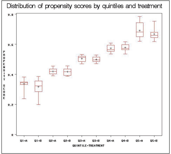
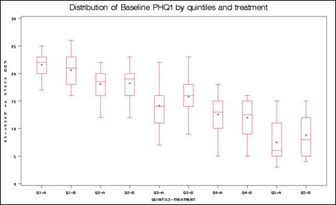
PROC BOXPLOT in Program 2.4 produces box plots of the propensity score distributions for each treatment group within each propensity stratum. The within-strata box plots showed general agreement, with potential exceptions of strata 1 and 5. However, assessment of treatment by strata interaction in the analysis model did not suggest differential results in these strata. The box plot can also be used to assess the distributions of each continuous covariate by treatment group within each propensity score stratum. The box plots of the baseline PHQ1 variable are provided in the output.
Macro GEN2 computes standardized differences for the unadjusted sample (without propensity scoring), averaged across propensity scores (adjusted) and within each propensity score stratum. The standardized differences are output to a data set so that summaries, listings, or box plots of the standardized differences can easily be created. Four of the five unadjusted standardized differences were greater than 0.10, while all of the standardized differences averaged over the strata were small. However, within-propensity score strata demonstrated many standardized differences greater than 0.10. While such differences are not greater than chance (as indicated by the two-way models), this does show the difficulty in producing and assessing balance with relatively small samples within each stratum. Balance in the propensity score does not necessarily mean balance in each individual covariate. Because of this, we examined other propensity models, including interactions as well as term removal. A model with significant two-way interactions and two-way interactions involving the PHQ1 term reduced the standardized differences, though modest imbalances were still noted in strata 1 and 5. Ultimately, variables other than PHQ1 did not appear strongly related to outcome, and the various models did not affect the outcome. One possible sensitivity analysis here would be to consider a propensity score matching analysis in order to obtain greater balance (see Chapter 3).
Macro GEN3 computes the weighted standardized differences for assessing covariate balance in a propensity score regression analysis. Output data sets from PROC GENMOD are used to compute the standardized differences and the MEANS procedure is used to summarize the data set with results from all the covariates. Both age and PHQ1 have standardized differences slightly greater than 0.1, indicating further assessment might be warranted. Adding these variables to the regression model as a sensitivity analysis once again did not result in any differences in the final results (OR=1.47; p=.235).
For this analysis, we assumed that there were no missing data for the covariate values, no dropouts, and no treatment changes (from A to B or from B to A) during the three months of the study. Chapter 5 covers computation of the propensity scores with missing covariate data, and Chapters 8 through 11 discuss methods used to address issues found in longitudinal naturalistic data.
In conclusion, various sensitivity analyses were all supportive of the initial analysis results. Thus, while unadjusted results suggested treatment differences, the propensity adjusted techniques revealed that the differences between treatments A and B on remission were not statistically significant.
Program 2.4 Evaluating Balance Produced by Propensity Score
/* This section of code evaluates the balance produced by the
propensity score by 1) summarizing the distribution of the propensity
scores via box plots, 2) running two-way models to compare the
balance of covariates before and after adjustment, and 3) computing
standardized treatment differences for each covariate before and
after adjustment. */
/*1. assessing balance between covariates by treatment and quintiles
of propensity scores by box plots*/
PROC FORMAT;
VALUE BPF 1 = 'Q1-A'
2 = 'Q1-B'
3 = 'Q2-A'
4 = 'Q2-B'
5 = 'Q3-A'
6 = 'Q3-B'
7 = 'Q4-A'
8 = 'Q4-B'
9 = 'Q5-A'
10 = 'Q5-B';
RUN;
DATA ADOS4;
SET ADOS3;
LABEL BP='QUINTILE-TREATMENT';
FORMAT BP BPF.;
IF TX=1 AND QUINTILES_PS=0 THEN BP=1;
ELSE IF TX=0 AND QUINTILES_PS=0 THEN BP=2;
ELSE IF TX=1 AND QUINTILES_PS=1 THEN BP=3;
ELSE IF TX=0 AND QUINTILES_PS=1 THEN BP=4;
ELSE IF TX=1 AND QUINTILES_PS=2 THEN BP=5;
ELSE IF TX=0 AND QUINTILES_PS=2 THEN BP=6;
ELSE IF TX=1 AND QUINTILES_PS=3 THEN BP=7;
ELSE IF TX=0 AND QUINTILES_PS=3 THEN BP=8;
ELSE IF TX=1 AND QUINTILES_PS=4 THEN BP=9;
ELSE IF TX=0 AND QUINTILES_PS=4 THEN BP=10;
RUN;
PROC SORT DATA=ADOS4;
BY BP;
RUN;
TITLE 'Distribution of propensity scores by quintiles and treatment';
PROC BOXPLOT DATA=ADOS4;
PLOT PS*BP;
RUN;
TITLE 'Distribution of Baseline PHQ1 by quintiles and treatment';
PROC BOXPLOT DATA=ADOS4;
PLOT PHQ1*BP;
RUN;
***********************************************************;
* MACRO STRATA is called by MACRO GEN2 and computes the *;
* standardized differences for a given subgroup (quintile)*;
* of the data. *;
* Input Variables: *;
* DATAIN - analysis data set *;
* DATOUT - output data set containing standardized *;
* differences *;
* STRN - strata number *;
***********************************************************;
%MACRO GEN1(VAR,DST,LNK);
* Run main effect and ps-adjusted models using GENMOD,
output parameter estimates to data sets for compilation*;
PROC GENMOD DATA = ADOS3 DESCENDING;
CLASS TX;
MODEL &VAR = TX / DIST = &DST LINK = &LNK TYPE3;
ODS OUTPUT TYPE3 = TEST1;
TITLE2 'TESTING FOR COVARIATE BALANCE: WITHOUT PS';
TITLE3 "VAR: &VAR"; RUN;
PROC GENMOD DATA = ADOS3 DESCENDING;
CLASS TX QUINTILES_PS;
MODEL &VAR = TX QUINTILES_PS TX*QUINTILES_PS / DIST =
&DST LINK = &LNK TYPE3;
LSMEANS TX / DIFF;
ODS OUTPUT TYPE3 = TEST2;
ODS OUTPUT LSMEANS = TESTL1;
TITLE2 'TESTING FOR COVARIATE BALANCE: WITH PS';
TITLE3 "VAR: &VAR"; RUN;
DATA TEST1;
SET TEST1;
OVAR = "&VAR";
DUM = 1;
PVAL_TX_UNADJ = PROBCHISQ;
TSTAT_TX_UNADJ = CHISQ;
TSTATDF_TX_UNADJ = DF;
KEEP DUM OVAR TSTAT_TX_UNADJ TSTATDF_TX_UNADJ PVAL_TX_UNADJ;
DATA TEST2A;
SET TEST2;
IF SOURCE = 'tx';
OVAR = "&VAR";
DUM=1;
PVAL_TX_ADJ = PROBCHISQ;
TSTAT_TX_ADJ = CHISQ;
TSTATDF_TX_ADJ = DF;
KEEP DUM OVAR TSTAT_TX_ADJ TSTATDF_TX_ADJ PVAL_TX_ADJ;
DATA TEST2B;
SET TEST2;
IF SOURCE = 'tx*QUINTILES_PS';
OVAR = "&VAR";
DUM=1;
PVAL_TXPS_ADJ = PROBCHISQ;
TSTAT_TXPS_ADJ = CHISQ;
TSTATDF_TXPS_ADJ = DF;
KEEP DUM OVAR TSTAT_TXPS_ADJ TSTATDF_TXPS_ADJ PVAL_TXPS_ADJ;
DATA TEST2B;
SET TEST2;
IF SOURCE = 'tx*QUINTILES_PS';
OVAR = "↕";
DUM=1;
PVAL_TXPS_ADJ = PROBCHISQ;
TSTAT_TXPS_ADJ = CHISQ;
TSTATDF_TXPS_ADJ = DF;
KEEP DUM OVAR TSTAT_TXPS_ADJ TSTATDF_TXPS_ADJ PVAL_TXPS_ADJ;
PROC SORT DATA = TEST1; BY DUM; RUN;
PROC SORT DATA = TEST2A; BY DUM; RUN;
PROC SORT DATA = TEST2B; BY DUM; RUN;
DATA BPP_&VAR;
MERGE TEST1 TEST2A TEST2B;
BY DUM;
%MEND GEN1;
* Call GEN1 macro to assess balance for each covariate and summarize
output in single data set*;
ODS LISTING CLOSE;
%GEN1(GENDER, BIN, LOGIT); RUN;
%GEN1(SPOUSE, BIN, LOGIT); RUN;
%GEN1(WORK, BIN, LOGIT); RUN;
%GEN1(AGE, NOR, ID); RUN;
%GEN1(PHQ1, NOR, ID); RUN;
ODS LISTING;
DATA BPP_ALL;
SET BPP_GENDER BPP_SPOUSE BPP_WORK BPP_AGE BPP_PHQ1;
PROC PRINT DATA = BPP_ALL;
VAR OVAR TSTAT_TX_UNADJ PVAL_TX_UNADJ TSTAT_TX_ADJ
PVAL_TX_ADJ PVAL_TXPS_ADJ;
TITLE 'PROPENSITY STRAT. BALANCE ASSESSMNT: 2-WAY MODELS';
TITLE2 'TEST STATISTICS (TSTAT) AND PVALUES (PVAL) FOR
MODELS WITHOUT PROPENSITY';
TITLE3 'ADJUSTMENT (UANDJ) AND WITH PROPENSITY ADJUSTMENT
(ADJ)'; RUN;
***********************************************************;
* MACRO STRATA is called by MACRO GEN2 and computes the *;
* standardized differences for a given subgroup (quintile)*;
* of the data. *;
* Input Variables: *;
* DATAIN - analysis data set *;
* DATOUT - output data set containing standardized *;
* differences *;
* STRN - strata number *;
***********************************************************;
%MACRO STRAT(DATIN,DATOUT,STRN);
DATA ONE;
SET &DATIN;
IF QUINTILES_PS = &STRN;
DATA ONE_A ONE_B;
SET ONE;
IF TX = 1 THEN OUTPUT ONE_A;
IF TX = 0 THEN OUTPUT ONE_B;
DATA ONE_A;
SET ONE_A;
MN_A_&STRN = MN;
SD_A_&STRN = SD;
NUM_A_&STRN = NUM;
DUMM = 1;
KEEP MN_A_&STRN SD_A_&STRN NUM_A_&STRN DUMM;
DATA ONE_B;
SET ONE_B;
MN_B_&STRN = MN;
SD_B_&STRN = SD;
NUM_B_&STRN = NUM;
DUMM = 1;
KEEP MN_B_&STRN SD_B_&STRN NUM_B_&STRN DUMM;
* This step merges the summary stats for each treatment and
computes the pooled variances and then the standardized
difference. For binary data variances a percentage value
between .05 and .95 is used to avoid infinite values. *;
DATA &DATOUT;
MERGE ONE_A ONE_B;
BY DUMM;
MN_DIFF_&STRN = MN_A_&STRN - MN_B_&STRN;
MN2_A_&STRN = MAX(MN_A_&STRN,.05); MN2_A_&STRN =
MIN(MN2_A_&STRN,.95);
MN2_B_&STRN = MAX(MN_B_&STRN,.05); MN2_B_&STRN =
MIN(MN2_B_&STRN,.95);
IF &BNRY = 0 THEN SD_DIFF_&STRN = SQRT( 0.5*(
SD_A_&STRN**2 + SD_B_&STRN**2 ));
IF &BNRY = 1 THEN SD_DIFF_&STRN = SQRT( (MN2_A_&STRN*(1-
MN2_A_&STRN) + MN2_B_&STRN*(1-MN2_B_&STRN)) / 2 );
STDDIFF_&STRN = MN_DIFF_&STRN / SD_DIFF_&STRN;
%MEND STRAT;
************************************************************;
* MACRO GEN2 computes the standardized differences for a *;
* given covariate within each propensity score strata *;
* (by calling the MACRO STRAT), unadjusted in the full *;
* sample (without propensity scoring), and averaging *;
* across the propensity score strata (adjusted) *;
* INPUT VARIABLES: *;
* VAR - covariate to be evaluated *;
* BNRY - enter 1 for binary covariate, 0 for continuous *;
************************************************************;
%MACRO GEN2(VAR,BNRY);
* Generate summary statistics for entire sample using PROC SUMMARY and then compute the standardized difference for the unadjusted full sample *;
PROC SUMMARY DATA = ADOS3;
CLASS TX;
VAR &VAR;
OUTPUT OUT=SSTAT MEAN=MN STD=SD N=NUM;
DATA SSTAT1;
SET SSTAT;
IF TX = 1;
MEAN_A = MN;
SD_A = SD;
N_A = NUM;
DUMM = 1;
DATA SSTAT2;
SET SSTAT;
IF TX = 0;
MEAN_B = MN;
SD_B = SD;
N_B = NUM;
DUMM = 1;
PROC SORT DATA = SSTAT1; BY DUMM; RUN;
PROC SORT DATA = SSTAT2; BY DUMM; RUN;
DATA SSTATF;
MERGE SSTAT1 SSTAT2;
BY DUMM;
MN_DIFF = MEAN_A - MEAN_B;
SDP = SQRT( ( (SD_A**2) + (SD_B**2) ) / 2 );
MEAN_A2 = MAX(MEAN_A,.05); MEAN_A2 = MIN(MEAN_A2,.95);
MEAN_B2 = MAX(MEAN_B,.05); MEAN_B2 = MIN(MEAN_B2,.95);
IF &BNRY = 1 THEN SDP = SQRT( (MEAN_A2*(1-MEAN_A2) +
MEAN_B2*(1-MEAN_B2)) / 2 );
STDDIFF_UNADJ = MN_DIFF / SDP;
OVAR = "&VAR";
KEEP OVAR DUMM MN_DIFF SDP STDDIFF_UNADJ;
* Generate summary statistics for each propensity strata using PROC SUMMARY and then compute the standardized difference for each strata using STRAT macro *;
PROC SORT DATA = ADOS3; BY QUINTILES_PS; RUN;
PROC SUMMARY DATA = ADOS3;
BY QUINTILES_PS;
CLASS TX;
VAR &VAR;
OUTPUT OUT=PSSTAT MEAN=MN STD=SD N=NUM;
DATA PSSTAT;
SET PSSTAT;
IF TX = ' ' THEN DELETE;
%STRAT(PSSTAT,SD0,0); RUN;
%STRAT(PSSTAT,SD1,1); RUN;
%STRAT(PSSTAT,SD2,2); RUN;
%STRAT(PSSTAT,SD3,3); RUN;
%STRAT(PSSTAT,SD4,4); RUN;
DATA MRG;
MERGE SD0 SD1 SD2 SD3 SD4;
BY DUMM;
ADJ_DIFF = (MN_DIFF_0 + MN_DIFF_1 + MN_DIFF_2 + MN_DIFF_3
+ MN_DIFF_4) / 5;
* Create final data set with standardized differences from unadjusted, adjusted, and within each quintile approach. The unadjusted SD is used here rather than a pooled within SD across strata to provide a direct comparison with the unadjusted standardized difference. *;
DATA FINAL_&VAR;
MERGE MRG SSTATF;
BY DUMM;
STDDIFF_ADJ = ADJ_DIFF / SDP;
KEEP OVAR STDDIFF_UNADJ STDDIFF_ADJ STDDIFF_0 STDDIFF_1
STDDIFF_2 STDDIFF_3 STDDIFF_4 ;
%MEND GEN2;
* Compute the standardized difference for each covariate by running GEN2 macro and then compile results into a single data set for summarizing. *;
%GEN2(GENDER,1); RUN;
%GEN2(SPOUSE,1); RUN;
%GEN2(WORK,1); RUN;
%GEN2(AGE,0); RUN;
%GEN2(PHQ1,0); RUN;
DATA FINAL;
SET FINAL_GENDER FINAL_SPOUSE FINAL_WORK FINAL_AGE
FINAL_PHQ1;
PROC PRINT DATA = FINAL;
VAR OVAR STDDIFF_UNADJ STDDIFF_ADJ STDDIFF_0 STDDIFF_1
STDDIFF_2 STDDIFF_3 STDDIFF_4;
TITLE 'STANDARDIZED DIFFERENCES BEFORE PS ADJUSTMENT
(STAND_DIFF_UNADJ), AFTER PS ';
TITLE2 ' ADJUSTMENT AVERAGING ACROSS STRATA
(STAND_DIFF_ADJ), AND WITHIN EACH PS';
TITLE3 ' QUINTILE (STDDIFF_0… STDIFF_4)'; RUN;
***********************************************************;
* MACRO GEN3 assesses the balance produced by a propensity*;
* scoring for a propensity score regression analysis. *;
* Weighted standardized differences (Austin, 2007a) are *;
* produced for a given covariate. *;
* INPUT VARIABLES: *;
* DVAR - covariate to be evaluated *;
* BNR - enter 1 for binary variable, 0 for continuous *;
* DST - NOR for normal, BIN for binary variables *;
* LNK - ID for normal, LOGIT for binary variables *;
***********************************************************;
%MACRO GEN3(DVAR,BNR,DST,LNK);
* Run the two-way model and output parameter estimates *;
PROC GENMOD DATA = ADOS3;
CLASS TX;
MODEL &DVAR = TX PS TX*PS / DIST = &DST LINK = &LNK TYPE3;
LSMEANS TX / DIFF;
ODS OUTPUT PARAMETERESTIMATES = TEST11;
ODS OUTPUT MODELFIT = TEST111;
TITLE2 'TESTING FOR COVARIATE BALANCE: WITH PS'; RUN;
DATA TRT_EST (KEEP = DUM TRT0_EST) PS_EST (KEEP = DUM
PS_EST) TRTPS_EST (KEEP = DUM TRT0PS_EST) INTRCPT_EST
(KEEP = DUM INTRCPT_EST);
SET TEST11;
DUM = 1;
IF PARAMETER = 'tx' AND LEVEL1 = ’;A’ THEN DO;
TRT0_EST = ESTIMATE;
OUTPUT TRT_EST;
END;
IF PARAMETER = 'PS' THEN DO;
PS_EST = ESTIMATE;
OUTPUT PS_EST;
END;
IF PARAMETER = 'PS*tx' AND LEVEL1 = ’A’ THEN DO;
TRT0PS_EST = ESTIMATE;
OUTPUT TRTPS_EST;
END;
IF PARAMETER = 'Intercept' THEN DO;
INTRCPT_EST = ESTIMATE;
OUTPUT INTRCPT_EST;
END;
DATA TEST111;
SET TEST111;
IF CRITERION = 'Deviance';
SIGHAT = SQRT(VALUEDF);
DUM = 1;
KEEP DUM SIGHAT;
DATA EST;
MERGE TEST111 TRT_EST PS_EST TRTPS_EST INTRCPT_EST;
DUM = 1;
KEEP TRT0_EST PS_EST TRT0PS_EST INTRCPT_EST SIGHAT DUM;
* Merge parameter estimates with analysis data to allow computation of predicted values for each patient. *;
DATA ADOS3;
SET ADOS3;
DUM = 1;
PROC SORT DATA = ADOS3; BY DUM; RUN;
PROC SORT DATA = EST; BY DUM; RUN;
DATA ALL;
MERGE ADOS3 EST;
BY DUM;
* For each observation, compute the predicted value assuming each treatment group *;
PRED0 = INTRCPT_EST + TRT0_EST + PS_EST*PS +
TRT0PS_EST*PS;
PRED1 = INTRCPT_EST + PS_EST*PS;
* Compute the standardized difference for continuous and binary covariates *;
IF &BNR = 0 THEN DO;
TRTDIFF = TRT0_EST + TRT0PS_EST*PS;
STDDIFF = ABS(TRT0_EST + TRT0PS_EST*PS) / SIGHAT;
END;
IF &BNR = 1 THEN DO;
PRED0B = EXP(PRED0) / (1 + EXP(PRED0));
PRED1B = EXP(PRED1) / (1 + EXP(PRED1));
TRTDIFF = PRED0B - PRED1B;
STDDIFF = ABS( TRTDIFF / SQRT( (PRED0B*(1-PRED0B) +
PRED1B*(1-PRED1B)) / 2 ) );
END;
DATA OUT_&DVAR;
SET ALL;
STDDIFF_&DVAR = STDDIFF;
KEEP AGE PHQ1 GENDER SPOUSE WORK PS STDDIFF_&DVAR;
%MEND GEN3;
* Call GEN3 macro for each covariate to compute the weighted standardized differences and then combine the results into a single data set for reporting. *;
ODS LISTING CLOSE;
%GEN3(GENDER, 1, BIN, LOGIT); RUN;
%GEN3(SPOUSE, 1, BIN, LOGIT); RUN;
%GEN3(WORK, 1, BIN, LOGIT); RUN;
%GEN3(AGE, 0, NOR, ID); RUN;
%GEN3(PHQ1, 0, NOR, ID); RUN;
ODS LISTING;
DATA REGSTD;
SET OUT_GENDER OUT_SPOUSE OUT_WORK OUT_AGE OUT_PHQ1;
PROC MEANS DATA = REGSTD N MEAN STD MIN MAX;
VAR STDDIFF_GENDER STDDIFF_SPOUSE STDDIFF_WORK
STDDIFF_AGE STDDIFF_PHQ1;
TITLE 'Assessing Propensity Score Balance for PS
Regression Analyses';
TITLE2 'Summary of Weighted Standardized Differences for
all covariates'; RUN;
Output from Program 2.4
PROPENSITY STRATIFICATION BALANCE ASSESSMENT: 2-WAY MODELS
TEST STATISTICS (TSTAT) AND PVALUES (PVAL) FOR MODELS WITHOUT PROPENSITY
ADJUSTMENT (UANDJ) AND WITH PROPENSITY ADJUSTMENT (ADJ)
| TSTAT | PVAL TX | TSTAT | PVAL TX | PVAL | ||
| Obs | OVAR | TX UNADJ | UNADJ | TX ADJ | ADJ | TXPS ADJ |
| 1 | GENDER | 0.52574 | 0.46840 | 0.75414 | 0.38517 | 0.43693 |
| 2 | SPOUSE | 0.36448 | 0.54603 | 0.12642 | 0.72217 | 0.91679 |
| 3 | WORK | 1.83639 | 0.17537 | 0.26352 | 0.60771 | 0.39002 |
| 4 | AGE | 1.55113 | 0.21297 | 0.00735 | 0.93168 | 0.55912 |
| 5 | PHQ1 | 8.47659 | 0.00360 | 0.38192 | 0.53658 | 0.38868 |
STANDARDIZED DIFFERENCES BEFORE PS ADJUSTMENT (STAND_DIFF_UNADJ), AFTER PS
ADJUSTMENT AVERAGING ACROSS STRATA (STAND_DIFF_ADJ), AND WITHIN EACH PS
QUINTILE (STDDIFF_0 … STDIFF_4)
| STDDIFF | STDDIFF_ | STDDIFF_ | STDDIFF_ | STDDIFF_ | STDDIFF_ | STDDIFF_ | ||
| Obs | OVAR | UNADJ | ADJ | 0 | 1 | 2 | 3 | 4 |
| 1 | GENDER | -0.10472 | -0.027202 | -0.27458 | 0.09386 | 0.15247 | -0.30824 | 0.34522 |
| 2 | SPOUSE | -0.0872C | -0.038501 | -0.12512 | -0.23010 | 0.08454 | 0.14960 | -0.11032 |
| 3 | WORK | 0.19633 | 0.084570 | 0.47314 | -0.28228 | -0.01852 | 0.43424 | -0.17660 |
| 4 | AGE | -0.17919 | -0.012030 | -0.41389 | -0.11483 | 0.36707 | 0.12328 | -0.10241 |
| 5 | PHQ1 | -0.42270 | -0.055802 | 0.35965 | -0.03898 | -0.42395 | 0.16759 | -0.35988 |
Summary of Weighted Standardized Differences for all covariates
The MEANS Procedure
| Variable | N | Mean | Std Dev | Minimum | Maximum |
| STDDIFF GENDER | 192 | 0.0176960 | 0.0129160 | 0.000075936 | 0.0660873 |
| STDDIFF SPOUSE | 192 | 0.0520099 | 0.0343423 | 0.000088147 | 0.1374309 |
| STDDIFF WORK | 192 | 0.0167626 | 0.0052507 | 0.0042665 | 0.0233658 |
| STDDIFF AGE | 192 | 0.1976337 | 0.1329724 | 0.0018827 | 0.5687586 |
| STDDIFF PHQ1 | 192 | 0.1702790 | 0.1142801 | 0.0039389 | 0.4802105 |
This chapter presents the stratification and regression methods for conducting a propensity score analysis. We have demonstrated how these analyses are conducted and discussed how to assess the quality of the propensity adjustment, the sensitivity analyses, and the differences from classical regression modeling. Finally, we have illustrated the details of the methods using SAS code applied to data from an observational study. In summary, propensity scores are a valuable approach for estimating the causal effects of exposures in naturalistic data.
The authors gratefully acknowledge the help of Josep Maria Haro.
Austin P. C., and M. M. Mamdani. 2006. “A comparison of propensity score methods: a case-study estimating the effectiveness of post-AMI statin use.” Statistics in Medicine 25(12): 2084—;106.
Austin P. C., P. Grootendorst, and G. M. Anderson. 2007a. “A comparison of the ability of different propensity score models to balance measured variables between treated and untreated subjects: a Monte Carlo study.” Statistics in Medicine 26(4): 734—;53.
Austin P. C., P. Grootendorst, S. T. Normand, and G. M. Anderson. 2007b. “Conditioning on the propensity score can result in biased estimation of common measures of treatment effect: a Monte Carlo study.” Statistics in Medicine 26: 754—;768.
Austin, P. C. 2008. “Goodness-of-fit diagnostics for the propensity score model when estimating treatment effects using covariate adjustment with the propensity score.” Pharmacoepidemiology and Drug Safety 17(12): 1202—;1217.
Braitman, L. E., and P. R. Rosenbaum. 2002. “Rare outcomes, common treatments: analytic strategies using propensity scores.” Annals of Internal Medicine 137(8): 693—;695.
Brookhart , M. A., S. Schneeweiss, K. J. Rothman, R. J. Glynn, J. Avorn, and T. StÜrmer. 2006. “Variable selection for propensity score models.” American Journal of Epidemiology 163(12): 1149—;1156.
Cadarette, S. M., J. N. Katz, M. A. Brookhart, T. StÜrmer, M. R. Stedman, and D. H. Solomon. 2008. “Relative effectiveness of osteoporosis drugs for preventing nonvertebral fracture.” Annals of Internal Medicine 148(9): 637—;646.
Cepeda, M. S., R. Boston, J. T. Farrar, and B. L. Strom. 2003. “Comparison of logistic regression versus propensity score when the number of events is low and there are multiple confounders.” American Journal of Epidemiology 158(3): 280—;287.
Cochran, W. G. 1968. “The effectiveness of adjustment by subclassification in removing bias in observational studies.” Biometrics 24: 295—;313.
D’Agostino, Jr., R. B., and R. B. D’Agostino, Sr. 2007. “Estimating treatment effects using observational data.” The Journal of the American Medical Association 297(3): 314—;316.
D’Agostino, R. B. 1998. “Propensity score methods for bias reduction in the comparison of a treatment to a non-randomized control group.” Statistics in Medicine 17 (19): 2265—;2281.
Grimes D. A., and K. F. Schulz. 2002. “An overview of clinical research: the lay of the land.” The Lancet 359: 57—;61.
Haro, J. M., S. Kontodimas, M. A. Negrin, M. D. Ratcliffe, D. Suarez, and F. Windmeijer. 2006. “Methodological aspects in the assessment of treatment effects in observational health outcomes studies.” Applied Health Economics & Health Policy 5 (1): 11—;25.
Hernán, M. A. 2004. “A definition of causal effect for epidemiological research.” Journal of Epidemiology and Community Health 58 (4): 265—;271.
Hernán, M. A., and J. M. Robins. 2006a. “Estimating causal effects from epidemiological data.” Journal of Epidemiology and Community Health 60 (7): 578—;586. (a)
Hernán, M. A., and J. M. Robins. 2006b. “Instruments for causal inference: an epidemiologist’s dream?” Epidemiology 17(4): 360—;372.
Imbens, G. W. 2000. “The role of the propensity score in estimating dose-response functions.” Biometrika 87 (3): 706—;710.
Joffe, M. M., and P. R. Rosenbaum. 1999. “Invited commentary: propensity scores.” American Journal of Epidemiology 150(4): 327—;333.
Kurth, T., A. M. Walker, R. J. Glynn, K. A. Chan, et al., 2006. “Results of multivariable logistic regression, propensity matching, propensity adjustment, and propensity-based weighting under conditions of nonuniform effect.” American Journal of Epidemiology 163(3):
262—;270.
Lunceford, J. K., and M. Davidian. 2004. “Stratification and weighting via the propensity score in estimation of causal treatment effects: a comparative study.” Statistics in Medicine 23 (19): 2937—;2960.
Martens, E.P., W. R. Pestman, A. D. Boer, S. V. Belitser, and O. H. Klungel. 2008. “Systematic differences in treatment effect estimates between propensity score methods and logistic regression.” International Journal of Epidemiology 37(5): 1142—;1147.
McCandless, L. C., P. Gustafson, and A. Levy. 2007. “Bayesian sensitivity analysis for unmeasured confounding in observational studies.” Statistics in Medicine 26: 2331—;2347.
McKee, M., A. Britton, N. Black, K. McPherson, et al. 1999. “Interpreting the evidence: choosing between randomised and non-randomised studies.” British Medical Journal 319: 312—;315.
Rosenbaum, P. R. 2002. Observational Studies. New York: Springer-Verlag.
Rosenbaum, P. R., and D. B. Rubin. 1983. “The central role of the propensity score in observational studies for causal effects.” Biometrika 70 (1): 41—;55.
Rosenbaum, P. R., and D. B. Rubin. 1984. “Reducing bias in observational studies using subclassification on the propensity score.” Journal of the American Statistical Association 79: 516—;524.
Rothwell, P. M. 2005. “Testing individuals 1: external validity of randomised controlled trials: “to whom do the results of this trial apply?” The Lancet 365(9453): 82—;93.
Rubin, D. B. 2007. “The design versus the analysis of observational studies for causal effects: parallels with the design of randomized trials.” Statistics in Medicine 26: 20—;36.
Schneeweiss, S. 2006. “Sensitivity analysis and external adjustment for unmeasured confounders in epidemiologic database studies of therapeutics.” Pharmacoepidemiology and Drug Safety 15 (5): 291—;303.
Senn, S. , E. Graf, and A. Caputo. 2007. “Stratification for the propensity score compared with linear regression techniques to assess the effect of treatment or exposure.” Statistics in Medicine 26 (30): 5529—;5544.
Setoguchi, S., S. Schneeweiss, M. A. Brookhart, R. J. Glynn, and E. F. Cook. 2008. “Evaluating uses of data mining techniques in propensity score estimation: a simulation study.” Pharmacoepidemiology and Drug Safety 17(6): 546—;555.
Shah, B. R., A. Laupacis, J. E. Hux, and P. C. Austin. 2005. “Propensity score methods gave similar results to traditional regression modeling in observational studies: a systematic review.” Journal of Clinical Epidemiology 58(6): 550—;9.
StÜrmer, T., M. Joshi, R. J. Glynn, J. Avorn, K. J. Rothman, and S. Schneeweiss. 2006. “A review of the application of propensity score methods yielded increasing use, advantages in specific settings, but not substantially different estimates compared with conventional multivariable methods.” Journal of Clinical Epidemiology 59 (5): 437.e1—;437.e24.
StÜrmer, T., S. Schneeweiss, J. Avorn, and R. J. Glynn. 2005. “Adjusting effect estimates for unmeasured confounding with validation data using propensity score calibration.” American Journal of Epidemiology 162: 279—;289.
Weitzen, S. , K. L. Lapane, A. Y. Toledano, A. L. Hume, and V. Mor. 2004. “Principles for modeling propensity scores in medical research: a systematic literature review.” Pharmacoepidemiology and Drug Safety 13 (12): 841—;853.
Weitzen, S., K. L. Lapane, A. Y. Toledano, A. L. Hume, and V. Mor. 2005. “Weaknesses of goodness-of-fit tests for evaluating propensity score models: the case of the omitted confounder.” Pharmacoepidemiology and Drug Safety 14 (4): 227—;238.
Woo, M. J., J. P. Reiter, and A. F. Karr. 2008. “Estimation of propensity scores using generalized additive models.” Statistics in Medicine 27(19): 3805—;3816.