
In this chapter, we look at autoencoders. This chapter is a theoretical one, covering the mathematics and the fundamental concepts of autoencoders. We discuss what they are, what their limitations are, the typical use cases, and then look at some examples. We start with a general introduction to autoencoders, and we discuss the role of the activation function in the output layer and the loss function. We then discuss what the reconstruction error is. Finally, we look at typical applications, such as dimensionality reduction, classification, denoising, and anomaly detection.
Introduction

Where in general xi ∈ ℝn with n ∈ ℕ. Autoencoders were introduced1 by Rumelhart, Hinton, and Williams in 1986 with the goal of “learning to reconstruct the input observations xi with the lowest error possible”.2
Why would you want to learn to reconstruct the input observations? If you have problems imagining what that means, think of having a dataset made of images. An autoencoder is an algorithm that can give as output an image that is as similar as possible to the input one. You may be confused, as there is no apparent reason to do this. To better understand why autoencoders are useful, we need a more informative (although not fully unambiguous) definition.
An autoencoder is a type of algorithm with the primary purpose of learning an “informative” representation of the data that can be used for different applications3 by learning to reconstruct a set of input observations well enough.
To better understand autoencoders, we need to refer to their typical architecture, visualized in Figure 9-1. The autoencoders’ main components are an encoder, a latent feature representation, and a decoder. The encoder and decoder are simply functions, while the latent feature representation typically means a tensor of real numbers (more on that later). Generally speaking, we want the autoencoder to reconstruct the input well enough. Still, at the same time, it should create a latent representation (the output of the encoder part in Figure 9-1) that is useful and meaningful.

The general structure of an autoencoder
In most typical architectures, the encoder and the decoder are neural networks5 (that is the case we will discuss at length in this chapter) since they can be easily trained with existing software libraries such as TensorFlow or PyTorch with backpropagation.

Where hi ∈ ℝq (the latent feature representation) is the output of the encoder block in Figure 9-1, when we evaluate it on the input xi. Note that we will have g : ℝn → ℝq.
 ) can be written then as a second generic function f of the latent features
 . Training an autoencoder simply means finding the functions g(·) and f(·) that satisfy
Where Δ indicates a measure of how the input and output of the autoencoder differ (basically our loss function will penalize the difference between the input and output) and < · > indicates the average over all observations. Depending on how you design the autoencoder, it may be possible to find f and g so that the autoencoder learns to reconstruct the output perfectly, thus learning the identity function. This is not very useful, as we discussed at the beginning of the chapter, and to avoid this possibility, two main strategies can be used: creating a bottleneck and adding regularization in some form.
We want the autoencoder to reconstruct the input well enough. Still, at the same time, it should create a latent representation (the output of the encoder) that is useful and meaningful.
Adding a “bottleneck,” (more on that later) is achieved by making the latent feature’s dimensionality lower (often much lower) than the input’s. That is the case that we look at in detail in this chapter. But before looking at this case, let’s briefly discuss regularization.
Regularization in Autoencoders

In the formula, the θi are the parameters in the functions f(·) and g(·) (you can imagine that in the case where the functions are neural networks, the parameters will be the weights). This is typically easy to implement, because the derivative with respect to the parameters is easy to calculate. Another trick that is worth mentioning is to tie the weights of the encoder to the weights of the decoder6 (in other words, make them equal). Those techniques, and a few others that go beyond the scope of this book, have fundamentally the same effect: to add sparsity to the latent feature representation.
We turn now to a specific type of autoencoders: those that build f and g with feed-forward networks that use a bottleneck. The reason for this choice is that they are very easy to implement and are very effective.
Feed-Forward Autoencoders

A typical architecture of a Feed-Forward Autoencoder. The number of neurons in the layers at first goes down as we move through the network, until it reaches the middle and then starts to grow again, until the last layer has the same number of neurons as the input dimensions
A typical FFA architecture (although it’s not mandatory) has an odd number of layers and is symmetrical with respect to the middle layer. Typically, the first layer has a number of neurons n1 = n (the size of the input observation xi). As we move toward the center of the network, the number of neurons in each layer drops in some measure. The middle layer (remember we have an odd number of layers) usually has the smallest number of neurons. The fact that the number of neurons in this layer is smaller than the size of the input is the bottleneck mentioned earlier.
In almost all practical applications, the layers after the middle one are a mirrored version of the layers before the middle one. For example, an autoencoder with three layers could have the following numbers of neurons: n1 = 10, n2 = 5 and then n3 = n1 = 10 (supposing we are working on a problem where the input dimension is n = 10). All the layers, up to and including the middle one, make what is called the encoder, and all the layers from and including the middle one (up to the output) make what is called the decoder
, as you can see in Figure 9-2. If the FFA training is successful, the result will be a good approximation of the input, in other words  . What is essential to notice is that the decoder can reconstruct the input by using only a much smaller number (q) of features than the input observations initially have (n). The output of the middle layer hi is also called a learned representation
of the input observation xi.
. What is essential to notice is that the decoder can reconstruct the input by using only a much smaller number (q) of features than the input observations initially have (n). The output of the middle layer hi is also called a learned representation
of the input observation xi.
The encoder can reduce the number of dimensions of the input observation (n) and create a learned representation (hi) of the input that has a smaller dimension q < n. This learned representation is enough for the decoder to reconstruct the input accurately (if the autoencoder training was successful as intended).
Activation Function of the Output Layer
In autoencoders based on neural networks, the output layer’s activation function plays a particularly important role. The most used functions are ReLU and sigmoid. Let’s look at both and see some tips on when to use which as well as why you should choose one instead of the other.
ReLU

It’s a good choice when the input observations xi assume a wide range of positive values.
If the input xi can assume negative values, the ReLU is a terrible choice, and the identity function is a much better choice.
The ReLU activation function for the output layer is well suited for cases when the input observations xi assume a wide range of positive, real values.
Sigmoid

This activation function can only be used if the input observations xi are all in the range ]0, 1[ or if you have normalized them to be in that range. Consider as an example the MNIST dataset. Each value of the input observation xi (one image) represents the gray values of the pixels that can assume any value from 0 to 255. Normalizing the data by dividing the pixel values by 255 would make each observation (each image) have only pixel values between 0 and 1. In this case, the sigmoid would be a good choice for the output layer’s activation function.
The sigmoid activation function for the output layer is a good choice in all cases where the input observations assume only values between 0 and 1 or if you have normalized them to assume values in the range ]0, 1[.
The Loss Function
 . If you remember the explanations at the beginning, you will realize that this loss function will be
Where for FFAs, g, and f will be the functions that are obtained with dense layers, as discussed in the previous sections. Remember that an autoencoder is trying to learn an approximation of the identity function; therefore, you want to find the weights in the network that give you the smallest difference according to some metric (Δ(·)) between xi and  . Two loss functions are widely used for autoencoders: Mean Squared Error (MSE) and Binary Cross-Entropy (BCE). Let’s look more in-depth at both since they can only be used when specific requirements are met.
Mean Square Error

The symbol ∣ · ∣ indicates the norm of a vector,8 and M is the number of the observations in the training dataset. It can be used in almost all cases, independently of how you choose your output layer activation function or how you normalize the input data.
It is easy to show that the minimum of LMSE is found for  . To prove it, let’s calculate the derivative of LMSE with respect to a specific observation, j. Remember that the minimum is found when this condition
is met for all i = 1, …, M. To simplify the calculations, let’s assume that the inputs are one dimensional9 and let’s indicate them with xi. We can write

 as can be easily seen, as we wanted to prove. To be precise, we also need to show that

This is greater than zero, therefore confirming our assumption that for  we indeed have a minimum.
Binary Cross-Entropy
If the activation function of the output layer of the FFA is a sigmoid function, thus limiting neuron outputs to be between 0 and 1, and the input features are normalized to be between 0 and 1, we can use the binary cross-entropy as a loss function, indicated here with LCE. Note that this loss function is typically used in classification problems, but it works beautifully for autoencoders. The formula for it is

Where xj, i is the jth component of the ith observation. The sum is over the entire set of observations and over all the components of the vectors. Can we prove that minimizing this loss function is equivalent to reconstructing the input as well as possible? Let’s calculate where LCE has a minimum with respect to  . In other words, we need to find out which values should
  assume to minimize LCE. As we have done for the MSE, to make the calculations easier, let’s consider the simplified case where xi and
  are one-dimensional and let’s indicate them with xi and
  .
.
To find the minimum of a function, as you should know from calculus, we need the first derivative of LCE. In particular, we need to solve the set of M equations

In this case, it is easy to show that the binary cross-entropy LCE is minimized when  for i = 1, …, M. Note that strictly speaking, this is true only when xi is different than 0 or 1 since
  can be neither 0 nor 1.
To find when the LCE is minimized, we can derive LCE with respect to a specific input 

Now remember that we need to satisfy the condition

 , as can be seen in Equation (9.3). To make sure that this is a minimum, we need to evaluate the second derivative. Since the point for which the first derivative is zero is a minimum only if
We can calculate the second derivative at the minimum point  easily

![$$ ilde{x}_{j}in left]0,1
ight[ $$](https://imgdetail.ebookreading.net/2023/10/9781484280201/9781484280201__9781484280201__files__images__463356_2_En_9_Chapter__463356_2_En_9_Chapter_TeX_IEq18.png) . We can immediately see that the denominator of the previous formula is greater than zero. The nominator is also clearly greater than zero since
. We can immediately see that the denominator of the previous formula is greater than zero. The nominator is also clearly greater than zero since  . Dividing two positive numbers gives a positive number, thus we have just proved that
The minimum of the cost function is reached when the output is exactly equal to the inputs, as we wanted to prove .
An essential prerequisite of using the binary cross-entropy loss function is that the inputs must be normalized between 0 and 1 and the activation function for the last layer must be a sigmoid or softmax function.
The Reconstruction Error


An example of big and small reconstruction errors when an autoencoder tries to reconstruct an image
Example: Reconstructing Handwritten Digits

In the top line, you can see the original digits from the MNIST dataset. In contrast, the bottom line contains the digits reconstructed by the autoencoder with the number of neurons equal to (784, 16, 784)
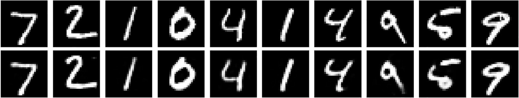
In the top line you can see the original digits from the MNIST dataset. The bottom line shows the digits reconstructed by the autoencoder with the number of neurons equal to (784, 64, 784)
This tells us that the relevant information on how to write digits is contained in a much lower number of features than 784.
An autoencoder with a middle layer smaller than the input dimensions (a bottleneck) can be used to extract the essential features of an input dataset. This creates a learned representation of the inputs given by the function g(xi). Effectively an FFA can be used to perform dimensionality reduction.

In the top line you can see the original digits from the MNIST dataset. In contrast, the bottom line contains the digits reconstructed by the autoencoder with the number of neurons equal to (784, 8, 784)

In the top line, you can see the original digits from the MNIST dataset. The second line of digits contains the digits reconstructed by the FFA (784,8,784). The third line is by the FFA (784,16,784), and the last line is by the FFA (784,64,784)
From Figure 9-7 you can see how, by increasing the middle layer’s size, the reconstruction gets better and better, as we expected.

In the top line, you can see ten random original digits from the MNIST dataset. The second line of digits contains the digits reconstructed with an FFA with 16 neurons in the middle layer and the binary cross-entropy as the loss function. The last line contains images reconstructed with the MSE as a loss function
Autoencoder Applications
Dimensionality Reduction
As mentioned in this chapter , using the bottleneck method, the latent features will have a dimension q that is smaller than the dimensions of the input observations n. The encoder part (once trained) does natural (by design) dimension reduction, thereby producing q real numbers. You can use the latent features for various tasks, such as classification (as you will see in the next section) or clustering.
We would like to point out some of the advantages of dimensionality reduction with an autoencoder compared to a more classical PCA approach. The autoencoder has one main benefit from a computational point of view: it can deal with a very large amount of data efficiently since its training can be done with mini-batches, while PCA, one of the most used dimensionality reduction algorithms, needs to do its calculations using the entire dataset. PCA is an algorithm that projects a dataset on the eigenvectors of its covariance matrix,13 thus providing a linear transformation of the features Autoencoders are more flexible and consider non-linear transformations of the features. The default PCA method uses  space for data in ℝd. This is, in many cases, not computationally feasible, and the algorithm does not scale up with increasing dataset size. This may seem irrelevant, but in many practical applications, the amount of data and the number of features is so big that PCA is not a practical solution from a computational point of view.
The use of an autoencoder for dimensionality reduction has one main advantage from a computational point of view: it can deal with a very large amount of data efficiently since its training can be done with mini-batches.
Equivalence with PCA
You use a linear function for the encoder g(·)
You use a linear function for the decoder f(·)
You use the MSE for the loss function
- You normalize the inputs to

The proof is long and can found in the notes by M.M. Kahpra for the course CS7015 (Indian Institute of Technology Madras) at http://toe.lt/1a.
Classification
Classification with Latent Features
The Different Accuracies and Running Times When Applying the kNN Algorithm to the Original 784 Features or the Eight Latent Features for the MNIST Dataset
Input Data | Accuracy | Running Time |
|---|---|---|
Original dataxi ∈ ℝ784 | 96.4% | 1000 sec. ≈16.6 min. |
Latent Features g(xi) ∈ ℝ8 | 89% | 1.1 sec. |
Using eight features allows us to get very good accuracy in just one second.
The Difference in Accuracy and Running Time When Applying the kNN Algorithm to the Original 784 Features with an FFA with Eight Neurons and with an FFA with 16 Neurons for the Fashion MNIST Dataset
Input Data | Accuracy | Running Time |
|---|---|---|
Original data xi ∈ ℝ784 | 85.4% | 1040 sec. ≈16.6 min. |
Latent Features enc(xi) ∈ ℝ8 | 79.9% | 1.2 sec. |
Latent Features enc(xi) ∈ ℝ16 | 83.6% | 3.0 sec. |
It is exciting to note that with an FFA with 16 neurons in the middle layer, we reach an accuracy of 83.6% in just three sec. When applying a kNN algorithm to the original features (784), we get an accuracy only 1.8% higher but with a running time of around 330 times longer.
Using autoencoders and doing classification with the latent features is a good way to reduce the training time by several orders of magnitude while incurring a minor drop in accuracy.
The Curse of Dimensionality: A Small Detour

The Length l of the Smallest Hyper-Cube to Contain at Least One Point from a Population of Randomly Distributed m Points
d | l |
|---|---|
2 | 0.003 |
10 | 0.50 |
100 | 0.93 |
1000 | 0.99 |
Furthermore, as you can see, the data becomes so sparse in high dimensions that you need to consider the entire hyper-cube to capture one single observation. When the data becomes so sparse, the number of observations you need in order to train an algorithm properly becomes much bigger than the size of existing datasets.

You can see that this number is very small for high values of d. For example, if we consider d = 100 it’s easy to see that we would need more observations than atoms in the universe17 to find at least one observation in that small portion of the hyper-cube.
Performing dimensionality reduction is a viable method for reducing running time dramatically while incurring a small drop in accuracy. In high-dimensionality datasets, this becomes fundamental due to the curse of dimensionality.
Anomaly Detection
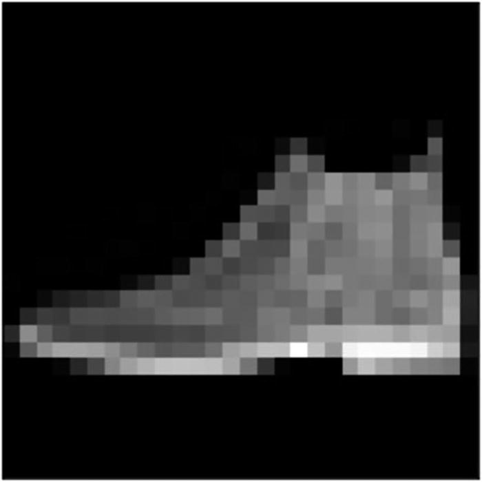
A random image from the Zalando MNIST dataset.
Let’s add it to the testing portion of the MNIST dataset. The original testing portion of MNIST has 10,000 images. With the shoe, we will have 10,001 images. How can we use an autoencoder to find the shoe automatically in those 10,001 images? Note that the shoe is an “outlier,” it’s an “anomaly” since it is an entirely different image class than handwritten digits. To do that, we will take the autoencoder we trained with the 60,000 MNIST images and calculate the reconstruction error for the 10,001 test images.

The shoe and the autoencoder's reconstruction trained on the 60,000 handwritten images of the MNIST dataset. This image has the biggest RE in the entire 10,001 test dataset we built, with a value of 0.062

The image with the second biggest RE in the 10,001 test dataset: 0.022
- 1.
Train an autoencoder on the entire dataset (or if possible, on a portion of the dataset known not to have an outlier).
- 2.
For each observation (or input) of the portion of the dataset known to have the wanted outliers, calculate the RE.
- 3.
Sort the observations by the RE.
- 4.
Classify the observations with the highest RE as outliers. The number of observations that classify as outliers will depend on the problem at hand and requires an analysis of the results (and usually a lot of knowledge of the data and the problem).
Note that if you train the autoencoder on the entire dataset, there is an essential assumption: the outliers are a negligible part of the dataset and their presence will not influence how the autoencoder learns to reconstruct the observations. This is one of the reasons that regularization is so essential. If the autoencoders could learn the identity function, anomaly detection could not be done.
A classic example of anomaly detection is finding fraudulent credit card transactions (the outliers). This case usually presents around 0.1% fraudulent transactions and therefore this would be a case that would allow us to train the autoencoder on the entire dataset. Another is fault detection in an industrial environment.
If you train the autoencoder on the entire dataset at disposal, there is an essential assumption: the outliers are a negligible part of the dataset and their presence will not influence how the autoencoder learns to reconstruct the observations.
Model Stability: A Short Note
Note that doing anomaly detection as described in the previous section seems easy, but those methods are prone to overfitting and often give inconsistent results. This means that training an autoencoder with a different architecture may well give different REs and therefore other outliers. There are several ways of solving this problem, but one of the simplest ways of dealing with instability of results is to train different models and then take the average of the REs. Another often used technique involves taking the maximum of the REs evaluated from several models. This kind of approaches are called ensemble methods but go beyond the scope of this book.
Anomaly detection done with autoencoders is prone to problems related to overfitting and unstable results. It is essential to be aware of these problems and check the results coming from different models to interpret the results correctly.
Note that this section serves to give you some pointers and is not meant to be an exhaustive overview on how to solve this problem.
Like autoencoders ensembles,18 more advanced techniques are also used to deal with problems of instable results coming, for example, from small datasets.
Denoising Autoencoders
Denoising autoencoders 19 are developed to auto-correct errors (noise) in the input observations. As an example, imagine the handwritten digits we considered before where we added some noise (for example, Gaussian noise) in the form of randomly changing the gray values of the pixels. In this case, the autoencoders should learn to reconstruct the image without the added noise. As a concrete example, consider the MNIST dataset. We can add to each pixel a random value generated by a normal distribution scaled by a factor (you can check out the code at https://adl.toelt.ai). We can train an autoencoder using the noisy images as the input and the original images as the output. The model should learn to remove the noise, since it is random in nature and has no relationship to the images.

The results of denoising an FFA autoencoder with three layers and 32 neurons in the middle layer . The noise was generated by adding a real number between 0 and 1 taken from a normal distribution. For details, see the code at https://adl.toelt.ai
Beyond FFA: Autoencoders with Convolutional Layers

A comparison of the results of an FAA (with architecture 784,32,784) and of a Convolutional Autoencoder (CA) with architecture (28x28), (26x26x64), (24x24,32), (26x26x64), (28x28)
Another important aspect is that the feature-generating layer can be a convolutional layer but can also be a dense one. There is no fixed rule and testing is required to find the best architecture for your problem. It also depends on how you want to model your latent features: as a tensor (multi-dimensional array) or as a one-dimensional array of real numbers.
Implementation in Keras
Where you can imagine that mnist_x_train and mnist_x_test are two datasets composed of several flattened MNIST handwritten digits. It is important to note that we have given the dataset mnist_x_train as input to the network for the images and for the output. In other words, there are no labels here. The labels are the dataset itself, since we want the output to be as close to the input as possible (remember the previous sections?).
At https://adl.toelt.ai you will find examples of autoencoders, anomaly detection with autoencoders, and denoising with autoencoders, as described in this chapter.
Exercises
List the most useful tasks you can use an autoencoder for. Can you think of an application in your field of work?
Can you explain briefly what a sparse autoencoder is? How is it similar to an autoencoder with a bottleneck?
How do you measure the performance of an autoencoder (which metric do you use)? List the most commonly used metrics that you can use. Can you think of any additional metric, in addition to those discussed in this chapter, that could be used?
Describe how anomaly detection works with autoencoders.
Further Readings
Deep Learning Tutorial from Stanford University
http://ufldl.stanford.edu/tutorial/unsupervised/Autoencoders/
Building autoencoders in Keras
https://blog.keras.io/building-autoencoders-in-keras.html
Introduction to autoencoders in TensorFlow
https://www.tensorflow.org/tutorials/generative/autoencoder
Bank, D., Koenigstein, N., and Giryes, R., “Autoencoders”, arXiv e-prints, 2020,
https://arxiv.org/abs/2003.05991
R. Grosse, University of Toronto, Lecture on autoencoders
http://www.cs.toronto.edu/~rgrosse/courses/csc321_2017/slides/lec20.pdf