
This chapter contains a basic introduction to the most important concepts of optimization and explains how they are related to neural networks. This chapter doesn’t go into detail, leaving longer discussions to the following chapters. But at the end of this chapter, you should have a basic understanding of the most important concepts and challenges related to neural networks. This chapter covers the problem of learning, constrained and unconstrained optimization problems, what optimization algorithms are, and the gradient descent algorithm and its variations (mini-batch and stochastic gradient descent).
A Basic Understanding of Neural Networks
 . The network function normally depends on a certain number N of parameters, which we will indicate with θi. We can write this mathematically as
 is as close to yi as possible. There are two very important undefined concepts in the last sentence: first, what “close” means, and second, how you update the parameters in an intelligent way to make
  and yi “close.” We answer those exact two questions in depth in this book.
A intuitive diagram of a neural network. xi are the inputs (for i = 1, …, M), θi are the parameters (for i = 1, …, N), and  is the output of the network. The network function is depicted by the irregular shape in the middle
To summarize, a neural network is nothing more than a mathematical function that depends on a set of parameters that are tuned, hopefully in some smart way, to make the network output as close as possible to some expected output. The concept of “close” is not defined here, but for the purposes of this section, a basic understanding is good enough. By the end of this book, you will have a more complete understanding of its meaning.
A neural network is nothing more than a mathematical function that depends on a set of parameters that are tuned, hopefully in some smart way, to make the network output as close as possible to some expected output.
The Problem of Learning
A First Definition of Learning
 with k being some integer. We will assume we have a set of M input observations with the expected target variables yi ∈ ℝk. We also assume that we have a mathematical function
  , called a loss function
, where we have used the vector notation y = (y1, …, yM),
, called a loss function
, where we have used the vector notation y = (y1, …, yM),  and θ = (θ1, …, θN). This function measures how “close” the expected (y) and predicted (
 ) values are, given specific values of the parameters θi. We will not yet define how this function looks, as this is not relevant for this discussion. Let’s summarize the notation we have defined so far:
xi ∈ ℝn: Input observations (for this discussion, we assume that they are a mono-dimensional array of dimension n ∈ ℕ). Examples could be age, weight, and height of a person, gray level values of pixels in an image, and so on.
yi ∈ ℝk: Target variables (what we want the neural network to predict). Examples could be the class of an image, what movie to suggest to a specific viewer, the translated version of a sentence in a different language, and so on.
f(θ, xi): Network function. This function is built with neural networks and depends on the specific architecture used (feed-forward, convolutional, recurrent, etc.).
θ = (θ1, …, θN): A set of real numbers, also called parameters or weights.
 : The loss or cost function. This function is a measure of how “close” y and
  are. Or, in other words, how good the neural network’s predictions are.
Those are the fundamentals elements that we need in order to understand neural networks.
[Advanced Section] Assumption in the Formulation
If you already have some experience with neural networks, it is important to discuss one important assumption that we have silently made. Note that skipping this short section in a first reading of this book will not impact the understanding of the rest. If you don’t understand the points discussed here, feel free to skip this part and come back to it later.
The most important assumption here can be found in how the loss function  is written. In fact, as written, it is a function of all the M components of the two vectors
  and y and this translates in not using a mini-batch during the training. The assumption here is that we will measure how good the network’s predictions are by considering all the inputs and outputs simultaneously. This assumption will be lifted in the following sections and chapters and discussed at length. The experienced reader may notice that this will lead to advanced optimization techniques—stochastic gradient descent and the concept of mini-batch. Using all the M components of the two vectors
  and y makes the learning process generally slower, although in some situations it’s more stable.
A Definition of Learning for Neural Networks
With the notation defined previously , we can now formally define learning in the context of neural networks.
 (the network function), and a function (the loss function)
  the process of learning is equivalent to minimizing the loss function with respect to the parameters θ. Or in mathematical notation
Learning is equivalent to minimizing the loss function with respect to the parameters θ, given a set of tuples (xi, yi) with i = 1, …M.
The typical term for learning is training and that is the one we will use in this book. Basically, training a neural network is nothing more than minimizing a very complicated function that depends on a very large number of parameters (sometimes billions). This presents very difficult technical and mathematical challenges that we discuss at length in this book. But for now, this understanding is sufficient to start understanding how to tackle this problem.
The following sections discuss how to solve the problem of minimizing a function in general and explain the fundamentals theoretical concepts that are necessary to understand more advanced topics. Note that the problem of minimizing a function is called an optimization problem .
Constrained vs. Unconstrained Optimization
The problem of minimizing a function as described in the previous section is called an unconstrained optimization problem .

Where ci(x) and qi(x) are constraint functions that define some equations and inequalities that need to be satisfied. In the context of neural networks, you may have the constraint that the output (suppose for a moment that  is simply a number) must lie in the interval [0, 1]. Or maybe that it must be always greater than zero or smaller than a certain value. Or another typical constraint that you will encounter is when you want the network to output only a finite number of outputs, for example, in a classification problem.
![$$ {hat{y}}_iin left[0,1
ight] $$](https://imgdetail.ebookreading.net/2023/10/9781484280201/9781484280201__9781484280201__files__images__463356_2_En_1_Chapter__463356_2_En_1_Chapter_TeX_IEq17.png) . Our learning problem could be formulated as follows
. Our learning problem could be formulated as follows

This is clearly a constrained optimization problem. When dealing with neural networks, this problem is typically reformulated by designing the neural network in such a way that the constraint is automatically satisfied, and learning is brought back to an unconstrained optimization problem.
[Advanced Section] Reducing a Constrained Problem to an Unconstrained Optimization Problem
You may be confused by the previous section and wonder how constraints can be integrated into the network architecture design. This happens typically in the output layer of the network. For example, in the examples discussed in the previous section, to ensure that  , it is enough to use the sigmoid function σ(s) as an activation function for the output neuron. This will guarantee that the network output will always be between 0 and 1 since the sigmoid function maps any real number to the open interval (0, 1). If the output of the neural network should always be 0 or greater, you could use the ReLU activation function for the output neuron.
When dealing with neural networks, constraints are typically built into the network architecture, thus reframing the original constrained optimization problem into an unconstrained one.
Building constraints into the network architecture is extremely useful and it typically makes the learning process much more efficient. Constraints often come from a deep knowledge of the data and the problem you are trying to solve. It pays off to find as many constraints as possible and to build them into the network architecture.

This is realized by having k neurons in the output layer and using for them the softmax activation function. This step reframes the problem into an unconstrained optimization problem, since the previous equation will be satisfied by the network architecture. If you don’t know what the softmax activation function is, don’t fret. We discuss it in the following chapters. Keep this example in mind, as it is the key to any classification problem with neural networks.
Absolute and Local Minima of a Function
![$$ exists eta in mathbb{R} mathrm{such} mathrm{that} f(x)le fleft({x}_0
ight)kern0.5em forall xin left[{x}_0-eta, {x}_0+eta
ight] $$](https://imgdetail.ebookreading.net/2023/10/9781484280201/9781484280201__9781484280201__files__images__463356_2_En_1_Chapter__463356_2_En_1_Chapter_TeX_Equg.png)
In principle, we want to find the global minimum or, in other words, the point for which the function value is the smallest between all possible points. In the case of neural networks, identifying if the minimum is a local or a global minimum is impossible, due to the network function complexity. This is one (albeit not the only one) of the reasons that training large neural networks is such a challenging numerical problem. In the next chapters, we discuss at length what factors2 may make finding the global minimum easier or more challenging.
Optimization Algorithms
So far, we have discussed the idea that learning is nothing less than minimizing a specific function, but we have not touched the issue of how this “minimizing” happens. This is achieved by what is called an “optimization algorithm,” whose goal it is to find the location of the (hopefully) absolute minimum. Practically speaking, all unconstrained minimization algorithms require the choice of a starting point, which you denote by x0. In the example of neural networks, this initial point would be the initial values of the weights. Typically starting from x0, the optimization algorithms will generate a sequence of iterates  that will converge toward the global minimum.
In all practical applications, only a finite number of terms will be generated, since we cannot generate an infinite number of xk of course. The sequence will stop when progress can no longer be made (the value of xk will not change any more3) or a specific solution has been reached with sufficient accuracy. Usually, the rule to generate a new xk will use information about the function f to be minimized and one or more previous values (often properly weighted) of the xk. In general, there are two main strategies for optimization algorithms: line search and trust regions. Optimizers for neural networks use all a line search approach.
Line Search and Trust Region


In the trust region approach , the information available on L is used to build a model function mk (typically quadratic in nature) that approximates f in a sufficiently small region around xk. Then this approximation is used to choose a new xk + 1. This book does not cover trust region approaches, but the interested reader can find a very complete introduction in Numerical Optimization, 2nd edition by J. Nocedal and S.J. Wright, published by Springer.
Steepest Descent


 ). Using the Taylor expansion and noting that f (xk) is a constant, we simply must solve for


as we claimed at the beginning.
The steepest descent method is a line-search method that searches for a better approximation of the minimum along the direction, minus the gradient of the function for every step. This method is at the basis of the gradient descent optimizer.
There are of course other directions that may be used, but for neural networks, those can be neglected. Just to cite an example, possibly the most important is the Newton direction, which can be derived from the second-order Taylor expansion of f(xk + p), but it requires you to know the Hessian ∇2L(x).
The Gradient Descent Algorithm


The Sequence xk Generated for the Function L(x) = x2 with the Parameters x0 = 1 and α = 0.1
k | xk x0 = 1 |
|---|---|
0 | 1 |
1 | 0.8 |
2 | 0.64 |
3 | 0.512 |
… | … |
40 | 0.00013 |
… | … |
500 | 3.5·10−49 |

 In Figure 1-2, you can see a plot of the sequence xk for various values of the parameter α.
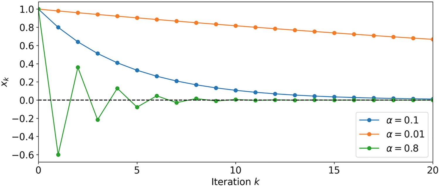
The sequence xk generated for the function L(x) = x2 for various values of α
 (green line), an oscillating sequence is generated. It is interesting to note how this oscillating sequence converges quite faster than the others. The value α = 1 generates a sequence that does not converge. But what happens for α > 1? This is a very interesting case, as it turns out that the sequence diverges (albeit oscillating from positive to negative values). In Figure 1-3, you can see the plot of the sequence for α = 1.01.
The sequence xk for the parameter α = 1.01. The sequence oscillates from positive to negative values while diverging in absolute value
You can clearly see how it diverges. Note that from a numerical point of view, it is easy to get NaN (if you are using Python) or errors. If you are trying neural networks and you get NaN for your loss function (for example), one possible reason may be a learning rate that is too big .
The learning rate is possibly one of the most important hyper-parameters that you have to decide on when training neural networks. Choose one that’s too small, and the training will be very slow, but choose one that’s too big, and the training will not converge! More advanced optimizers (Adam for example) try to compensate this shortcoming by effectively varying the learning rate6 dynamically, but the initial value is still important.

Therefore, it’s easy to see that this sequence converges for |1 − 2α| < 1 and diverges for |1 − 2α| > 1. For |1 − 2α| = 1, it stays at 1 and if 1 − 2α = − 1, it oscillates between 1 and −1. Still, it is instructive to see how important the role of the learning rate is when using the GD.
Choosing the Right Learning Rate
- 1.
Choose an initial learning rate. Typical values7 are 10−2 or 10−3.
- 2.
Let your optimizer run for a certain number of iterations, saving the L(xk) each time.
- 3.
Plot the sequence L(xk). This sequence should show a convergent behavior. From the plot, you can get an idea whether the learning is too small (slow convergence) or too big (divergence). For example, Figure 1-4 shows the sequence L(xk) for the example we discussed in the previous section. The figure tells us that using α = 0.01 (orange line) is very slow. Trying larger values for α shows how convergence can be faster (blue and green). With α = 0.1 after 12-13 iterations, you already have a good approximation of the minimum, while for α = 0.01 you are still very far from a solution.
When training neural networks, always check the behavior of your loss function. This will give you important information about how the training process is going.

The sequence L(xk) for the function L(x) = x2 for various values of α
This is why, when training neural networks, it is important to always check the behavior8 of the loss function that you are trying to minimize. Never assume that your model is converging without checking the sequence L(xk).
Variations of GD
 , where we have used the vector notation y = (y1, …, yM),
  and θ = (θ1, …, θN). In other words, we have at our disposal M input tuples that we can use. In the plain version of GD, the loss function is written as


That is the classical formula for the MSE that you may have already seen. In plain GD, we would use this formula to evaluate the gradient that we need to minimize L. Using all M observations has pros and cons.
Plain GD shows a stable convergence behavior
Usually, this algorithm is implemented in such a way that all the dataset must be in memory; therefore, it is computationally intensive.
This algorithm is typically very slow with very big datasets.
Variations of the GD are based on the idea of considering only some of the observations in the sum in the previous equation instead of all M. The two most important variations are called mini-batch GD (MBGD, where you consider a small number of observations m < M) and stochastic GD (SGD, where you consider only one observation at a time). Let’s look at both in detail, starting with the mini-batch GD.
Mini-Batch GD

Where we have introduced m ∈ ℕ with m < M, called batch size. Lm is defined by summing over m observations sampled from the initial dataset.
- 1.
A mini-batch size m is chosen. Typical values are 32, 64, 128, or 256 (note that the mini-batch size m does not have to be a power of 2, and it can be any number, such as 137 or 17).
- 2.
 subsets of observations are created9 by sampling each time m observation from the initial dataset S without repetition. We indicate them with
  . Note that in general if M is not a multiple of m the last batch,
  may have a number of observations smaller than m.
 - 3.
The parameters θ are updated Nb times using the GD algorithm with the gradient of Lm evaluated over the observations in Si for i = 1, …, Nb.
- 4.
Repeat Step 3 until the desired result is achieved (for example, the loss function does not vary much anymore).
When training neural networks, you may have heard the term “epoch” instead of iteration. An epoch is finished after all the data has been used in the previous algorithm. Let’s look at an example. Suppose we have M = 1000 and we choose m = 100. The parameters θ will be updated using 100 input observations each time. After ten iterations ( ) the network will have used all M observations for its training. At this point, it is said that one epoch is finished. One epoch in this example consists of ten times the parameters being updated (or ten iterations). Here are the advantages and disadvantages.
The parameters update frequency is higher than with plain gradient descent but lower than SGD, therefore allowing for a more robust convergence than SGD
This method is computationally much more efficient than plain gradient descent or Stochastic GD since fewer calculations (as in SGD) and resources (as in Plain GD) are needed.
This variation is by far the fastest of the three and the most commonly used.
The use of this variation introduces a new hyper-parameter that needs to be tuned: the batch size (the number of observations in the mini-batch).
An epoch is finished after all the input data has been used to update the parameters of the neural network. Remember that in one epoch, the parameters of the network may be updated many times.
Stochastic GD
SGD is a very common version of the GD, and it simply is the mini-batch version with m = 1. This involves updating the parameters of the network by using one observation at a time for the loss function. This also has advantages and disadvantages.
The frequent updates provide an easy way to check how the model learning is going (you don’t need to wait until all the dataset has been considered).
In a few problems this algorithm may be faster than plain gradient descent.
The model is intrinsically noisy and that may help the model avoid local minima when trying to find the absolute minimum of the cost function.
On large datasets, this method is quite slow, as it’s very computationally intensive due to the continuous updates.
The fact that the algorithm is noisy can make it hard for the algorithm to settle on a minimum for the cost function, and the convergence may not be as stable as expected.
How to Choose the Right Mini-Batch Size
So, what is the right mini-batch size m? Typical values used by practitioners are in the order of 100 or less. For example, the TensorFlow standard value (if you don’t specify otherwise) is 32. Why is this value so special? To understand why, you need to study the behavior of MBGD for various choices of m. To make it resemble real cases, consider the MNIST dataset. You may have already seen it. It is a dataset that contains 70,000 hand-written digits from 0 to 9. The images are gray-level 28x28 pixel images. We will build a classifier with a neural network with 16 neurons using the ReLU activation function and use the Adam optimizer. Note that if you don’t know what I am talking about, you can skip those details. The following discussion can be followed even without understanding the details of how the network is designed.
Secondly, using Adam is only for practical reasons, as in TensorFlow the MBGD is not available out of the box. But the conclusions continue to be valid. We have trained the network for ten epochs on 60,000 training images and then measured the running time10 needed, the reached value of the loss function, and the accuracy at the end of the training. We used the following values for the mini-batch size m: 60000 (effectively using all the data, so no mini-batches), 20000, 5000, 500, 50, 10, and 1. Note that while for m = 10 the required time is 2.34 min, when using m = 1, 19.18 minutes are needed for ten epochs!

A plot of the loss function reached after ten epochs on the MNIST dataset plotted vs. the running time needed. a indicates the accuracy reached
Let’s see what Figure 1-5 is telling us. When we use m = 60000, the running time needed for ten epochs is the lowest, but the accuracy is quite low. Decreasing m increases the accuracy quite rapidly, until we reach the “elbow.” Between m = 500 and m = 50, the behavior changes. Decreasing m does not increase the accuracy much, but the running time becomes larger and larger. So, when we reach the elbow, a decrease in m is no longer advantageous. As you will notice, around the elbow, m is in the order of 100. Figure 1-5 shows why typical values for m are in the order of 100. Of course, the optimal value is dependent on the data and some testing is required, but in most cases a value around 100 is a very good starting point.
A good starting point for the mini-batch size is in the order of 100. The optimal value is dependent on the data you use and on the neural network architecture you train, and testing is required to find the optimal value.
[Advanced Section] SGD and Fractals
![$$ {x}^{left[i
ight]}=left({x}_1^{left[i
ight]},{x}_2^{left[i
ight]}
ight)in {mathbb{R}}^2 $$](https://imgdetail.ebookreading.net/2023/10/9781484280201/9781484280201__9781484280201__files__images__463356_2_En_1_Chapter__463356_2_En_1_Chapter_TeX_IEq29.png) . We call the target variables y[i]. The optimization problem we are trying to solve involves minimizing this function
. We call the target variables y[i]. The optimization problem we are trying to solve involves minimizing this function![$$ L=frac{1}{2}sum limits_{i=1}^M{left(fleft({x}_1^{left[i
ight]},{x}_2^{left[i
ight]}
ight)-{y}^{left[i
ight]}
ight)}^2 $$](https://imgdetail.ebookreading.net/2023/10/9781484280201/9781484280201__9781484280201__files__images__463356_2_En_1_Chapter__463356_2_En_1_Chapter_TeX_Equy.png)
![$$ fleft({x}_1^{left[i
ight]},{x}_2^{left[i
ight]}
ight)={w}_1{x}_1^{left[i
ight]}+{w}_2 {x}_2^{left[i
ight]} $$](https://imgdetail.ebookreading.net/2023/10/9781484280201/9781484280201__9781484280201__files__images__463356_2_En_1_Chapter__463356_2_En_1_Chapter_TeX_Equz.png)


The calculations are boring but not overly complex. By solving these two equations, you will find that the minimum is at  .
.
Exercises

And prove that L has its global minimum at  .
.
- 1.
Choose a learning rate α.
- 2.
Choose a random value between {1,2,3} and assign it to i.
- 3.
Update the parameters w1, w2 by using
![$$ {l}_i=frac{1}{2}{left(fleft({x}_1^{left[i
ight]},{x}_2^{left[i
ight]}
ight)-{y}^{left[i
ight]}
ight)}^2 $$](https://imgdetail.ebookreading.net/2023/10/9781484280201/9781484280201__9781484280201__files__images__463356_2_En_1_Chapter__463356_2_En_1_Chapter_TeX_IEq32.png) ; in other words, use li to calculate the derivatives to update the weights according to the gradient descent rule wj → wj − α∂li/∂wj for j = 1, 2. Each time, save the values w1, w2, for example in a Python list.
; in other words, use li to calculate the derivatives to update the weights according to the gradient descent rule wj → wj − α∂li/∂wj for j = 1, 2. Each time, save the values w1, w2, for example in a Python list. - 4.
Repeat Steps 2 and 3 a certain number of times, N.

Each blue point is a tuple of values (w1, w2) that are generated by using SGD as described in the section for a value of the learning rate α = 0.65. The plot has been obtained using 4 · 105 iterations
Can you derive the equations of the lines delimiting the triangle from the input matrix X?
Try to reproduce the image by implementing the SGD algorithm as described in this section from scratch. If you are stuck, you can find a complete implementation in the online version of the book.

A zoomed region that shows the fractal nature that the SGD algorithm can generate. This picture has been generated with a learning rate of α = 0.65 and with 107 iterations. In the zoomed region, you can clearly see the same kind of structure that you observe at a larger scale on the left. The zoomed region is less sharp than the one on the left since only a fraction of the 107 points happen to be in the small regioned zoomed in

Fractal shapes obtained by SGD for different learning rates. Note in the figure the learning rate is indicated with γ.

By choosing smaller and smaller learning rates, the fractal structures completely disappear, leaving an unstructured cloud of points centered on the global minimum x∗ of L.

By choosing a very small learning rate of α = 5 · 10−4, SGD will move in the direction of the expected global minimum x∗ and remain in its vicinity, as can be seen in the zoomed-in region. Still, SGD continues to deliver points that remain around x∗, but never converge to it. The smaller the learning rate, the smaller the cloud of points around x∗
Prove that each of the updates done with SGD, as described in the previous section, moves the point in parameter space in the direction perpendicular to one of the three lines that describe the triangle in the previous figures. In other words, the direction between two subsequent updates of the parameters (w1, w2) and  is perpendicular to one of the three lines that delimitate the triangle in the previous figures. Note that this is not an easy exercise, and you can find some tips in the online version of the book if you get stuck.
The gradient descent algorithm, especially in its stochastic version, has incredible hidden complexity, even for a trivial case, as the one described in the previous section. This is the reason that training neural networks can be so difficult and tricky, and why choosing the right learning rate and optimizer is so important.
Conclusion
You should now have all the ingredients to (at least at a basic level) understand what it means for neural networks to learn. We have not yet covered how to build a neural network, except for the fact that it is a very complicated function f of the inputs that depend on a large number of parameters. We go into a lot more detail about how neurons work, how non-linearity is introduced, and so much more.
A neural network architecture, namely a way of getting from an input x to an answer
 (remember the function f ?) that can be tuned by changing a large number of parameters.
A set of input observations xk (possibly a large number of them) with the expected values we want to predict (we are dealing with supervised learning).
An optimizer, or in other words, an algorithm that can find the best parameters of the network to get the outputs as close as possible to what you expect.
This chapter discussed these points in a basic way. It is important that you get the main idea behind what training neural networks means. The next chapters discuss each of the three points in more detail and include a lot of examples to make the discussion as clear as possible. We build on what’s discussed here to bring you to a point where you can use these more advanced techniques for your projects.