What Are Recommendation Engines?

In the past, people generally purchased products recommended to them by their friends or the people they trust. This is how people used to make purchasing decisions when there was doubt about a product. But since the advent of the Internet, we are so used to ordering online and streaming music and movies that we are constantly creating data in the back end. A recommendation engine uses that data and different algorithms to recommend the most relevant items to users. It initially captures the past behavior of a user, and then it recommends items for future purchase or use.

There are scenarios where there is no historical data as well. For example, when a new user visits a site, there is no history of that user. So how does the website recommend products to this user? One way is by recommending bestselling products (i.e., the products that are trending). Another possible solution is to recommend the products that bring maximum profit to the business and any new products recently added to the site.

If you can recommend a few items to a customer based on their interests, it positively impacts the user experience and leads to frequent visits. Hence, intelligent recommendation engines are built by studying the past behavior of their users to enhance revenue.

Recommendation System Types

Data on a user’s likes and dislikes of items are essential to building a recommender engine that can suggest relevant items to the user. There are two feedback mechanisms through which users provide this required data.

Explicit feedback is the data that the user explicitly provides as feedback on an item. It is usually difficult to obtain this type of feedback from users, and companies try many innovative ways. A simple like or dislike button, star ratings, and even comments and reviews as text input can get user feedback on an item.

Implicit feedback is the data that the user implicitly or unknowingly provides through their actions. This can be in the form of pages visited, items viewed, the number of clicks, and all sorts of other activities performed on the site/platform, which can indicate their interest in certain items. This type of data is generally captured automatically through cookies and browsing history and doesn’t require any direct action from the users.

Types of Recommendation Engines

Market Basket Analysis (Association Rule Mining)

Retailers predominantly use market basket analysis to reveal relationships between items. It works by looking for combinations of items that are often put together, allowing retailers to identify relationships between items that people buy.

There are several terms used in association analysis that are important to understand. Association rules are widely used to analyze retail basket or transaction data. They are intended to identify strong rules discovered in transaction data using interest measures based on the concept of strong rules.

Association rules are normally written like this: {bread} -> {butter}. This means a strong relationship exists between customers who bought bread and butter in the same transaction.

In the preceding example, {bread} is the antecedent and {butter} is the consequent. Both antecedents and consequences can have multiple items. In other words, {bread, milk} -> {butter, chips} is a valid rule.

Support is the relative frequency of the rule display. In many cases, you may want to seek high support to make sure it’s a worthwhile relationship. However, there may be cases where low support is useful if you are trying to find “hidden” relationships.

Confidence is a measure of the reliability of a rule. A 0.5 reliability in the preceding example means that bread and milk were purchased 50% of the time. The purchase also included butter and chips. For a product recommendation, 50% confidence may be perfectly acceptable, but this level may not be high enough in a medical situation.

Lift is the ratio of observed support to expected support if the two rules were independent. As a rule of thumb, a lift value close to 1 means that the rules were completely independent. Lift - values > 1 are more “interesting” and could indicate a useful rule pattern. Figure 1-1 illustrates how support, confidence, and lift are calculated.

An analysis of market basket rules. It includes four rules with support, confidence, and lift calculations. The rules are 1. A implies D. 2. C implies A. 3. A implies C. 4. B and C imply D.

Content-Based Filtering

The content-based filtering method is a recommendation algorithm that suggests items similar to the ones the users have previously selected or shown interest in. It can recommend based on the actual content present in the item. For example, as shown in Figure 1-2, a new article is recommended based on the text present in the articles.

An illustration depicts a content-based filtering method. It reveals new articles recommended, based on the text present in the article (text read by the user and similar articles are recommended to other users).

Let’s look at the popular example of Netflix and its recommendations to explore the workings in detail. Netflix saves all user viewing information in a vector-based format, known as the profile vector, which contains information on past viewings, liked and disliked shows, most frequently watched genres, star ratings, and so forth. Then there is another vector that stores all the information regarding the titles (movies and shows) available on the platform, known as the item vector. This vector stores information like the title, actors, genre, language, length, crew info, synopsis, and so forth.

The content-based filtering algorithm uses the concept of cosine similarity. In it, you find the cosine of the angle between two vectors—the profile and item vectors in this case. Suppose A is the profile vector and B is the item vector, then the (cosine) similarity between them is calculated as follows.

A formula states: sim open parenthesis A, B close parenthesis equals cos theta equals start fraction A dot B over either A OR B end fraction, here A is the profile vector and B is the item vector.

A formula for Euclidean distance. The square root of x subscript 1 minus x subscript 1 whole square plus up to plus x subscript N minus y subscript N whole square.

• Pearson’s correlation refers to how correlated or similar two things are. The higher the correlation, the higher the similarity. Pearson’s correlation is calculated using the formula shown in Figure 1-3.

A formula for Pearson's correlation. Sim of u, v is equal to the summation of r subscript u i minus r superscript hyphen subscript u and r subscript v i minus r superscript hyphen subscript v over square root of summation of r subscript u i minus r superscript hyphen subscript u whole square and the square root of summation of r subscript v i minus r superscript hyphen subscript v whole square is the end of the formula.

The major downside to this recommendation engine is that all suggestions fall into the same category, and it becomes somewhat monotonous. As the suggestions are based on what the user has seen or liked, we’ll never get new recommendations that the user has not explored in the past. For example, if the user has only seen mystery movies, the engine will only recommend more mystery movies.

To improve on this, you need a recommendation engine that not only gives suggestions based on the content but also on the behavior of users and on what other like-minded users are watching.

Collaborative-Based Filtering

In collaborative-based filtering recommendation engines, a user-to-user similarity is also considered, along with item similarities, to address some of the drawbacks of content-based filtering. Simply put, a collaborative filtering system recommends an item to user A based on the interests of a similar user B. Figure 1-4 shows a simple working mechanism of collaborative-based filtering

An illustration depicts the collaborative-based filtering method. It recommends an item to user A based on the interests of a similar user B. Here displays an example with two users A and B.

The similarity between users can be calculated again by all the techniques mentioned earlier. A user-item matrix is created individually for each customer, which stores the user’s preference for an item. Taking the same example of Netflix’s recommendation engine, the user aspects like previously watched and liked titles, ratings provided (if any) by the user, frequently watched genres, and so on are stored and used to find similar users. Once these similar users are found, the engine recommends titles that the user has not yet watched but users with similar interests have watched and liked.

This type of filtering is quite popular because it is only based on a user’s past behavior, and no additional input is required. It’s used by many major companies, including Amazon, Netflix, and American Express.

One of the drawbacks of this method happens when no ratings are provided for a particular item; then, it can’t be recommended. And reliable recommendations can be tough to get if a user has only rated a few items.

Hybrid Systems

So far, you have seen how content-based and collaborative-based recommendation engines work and their respective pros and cons. But the hybrid recommendation system combines content and collaborative-based filtering methods.

Hybrid recommendation systems can overcome the drawbacks of both content-based and collaborative-based to form one powerful recommendation system, both the individual methods fail to perform well when there is a lack of data to learn the relation between users and items, which is overcome in this hybrid approach.

Figure 1-5 shows a simple working mechanism of the hybrid recommendation system.

A flow chart depicts the working mechanism of the hybrid recommendation system. It includes two inputs, one with C F-based recommender, the other with a content-based recommender, combiner, and R E C O.

Several studies compare the performance of conventional methods to that of a hybrid system, showing that hybrid recommender engines generally perform better and provide more reliable recommendations.

ML Clustering

In today’s world, AI has become an integral part of all automation and technology-based solutions and the area of recommendation systems is no different. Machine learning-based methods are the upcoming high prospective methods that are quickly becoming a norm as more and more companies start adapting AI.

Machine learning methods are of two types: unsupervised and supervised. This section discusses the unsupervised learning method, which is the ML clustering–based method. The unsupervised learning technique uses ML algorithms to find hidden patterns in data to cluster them without human intervention (unlabeled data). Clustering is the grouping of similar objects into clusters. On average, an object belonging to one cluster is more similar to an object within that cluster than to an object belonging to another cluster.

In recommendation engines, clustering is used to form groups of users similar to each other, as shown in Figure 1-6. It can also cluster similar items or products as well. Traditionally similarity measures like cosine similarity have been used to get similar users or items, but they have their demerits. If a user has not rated many items and the resultant user-item matrix is sparse, or when you need to compare multiple user-user pairings to find similar users, it gets computationally expensive. A clustering-based approach is generally taken to get similar users to overcome these issues. If a user is found to be similar to a cluster of users, that user is added to that cluster. Within the cluster, all users share interests and tastes, and recommendations are provided to users based on them.

A pie chart depicts the group-based similarity. It includes clustering to form groups of users similar to each other (cluster similar products or items).

The following are some of the popularly used clustering algorithms.

• k-means clustering

• fuzzy mapping

• self-organizing maps (SOM)

• a hybrid of two or more techniques

Rule-Based Recommendation Systems

You build these recommendation systems with simple rules, such as popularity-based or buy again.

Popularity

A popularity-based rule is the simplest form: a product is recommended based on its popularity (most sold, most clicked, etc.). Let’s implement a quick one. For example, a song listened to by many people means it’s popular. It is recommended to others without any other intelligence being part of it.

Let’s take a retail dataset and implement the same logic.

Fire up a Jupyter notebook and import the necessary packages.

#import necessary libraries

import pandas as pd

import numpy as np

#import viz libraries

import seaborn as sns

import matplotlib.pyplot as plt

%matplotlib inline

Let’s import the data.

Note Refer to the data in this book’s data section. Download the dataset from the GitHub link of this book.

#import data

df = pd.read_csv('data.csv',encoding= 'unicode_escape')

df.head()

Figure 1-7 shows the output of the top 5 rows from the dataset.

An output file depicts the popularity-based rule. It includes invoice number, stock code, description, quantity, invoice date, unit price, customer I D, and country. It has five rows of data.

# null value counts

df.isnull().sum().sort_values(ascending=False)

An output file depicts the null value counts. It includes customer I D, description, country (null), unit price (null), invoice date (null), quantity (null), stock code (null), invoice number (null), and d type.

# drop where Description is not available

df_new = df.dropna(subset=['Description'])

df_new.describe()

Figure 1-8 shows that the quantity has some negative values that are a part of the incorrect data, so lets drop them using the below code.

df_new = df_new[df_new.Quantity > 0]

df_new.describre()

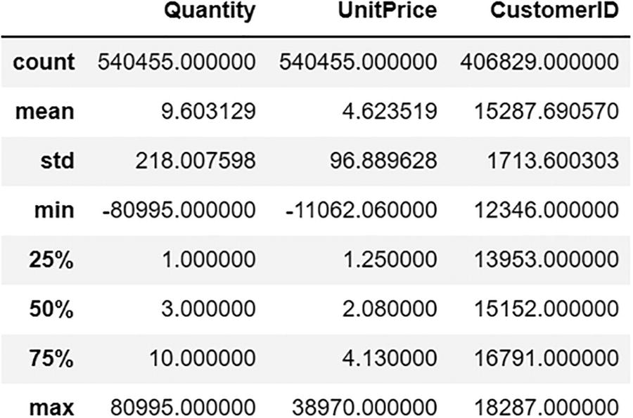
An output file depicts eight rows of data with some negative values (incorrect data). It includes quantity, unit price, and customer I D with two negative values in minimum.

An output file depicts eight rows of data with the popularity-based recommendation system. It includes quantity, unit price, and customer I D with count, mean, S T D, minimum, 25, 50, and 75 percent. Here 25 percent is highlighted.

Now that we cleaned up the data, let’s do some basic types of recommendation systems. These are not intelligent yet effective in some cases. Popularity-based recommendation systems could be a trending song. It could be a fast-selling item required for everyone, a recently released movie that gets traction, or a news article many users have read.

Sometimes it’s important to keep it simple because it gets you the most revenue. Let’s build a popularity-based system in the data we are using.

Global Popular Items

Let’s calculate popular items worldwide and then dice them into different regions.

# popular items globally

global_popularity=df_new.pivot_table(index=['StockCode','Description'], values='Quantity', aggfunc='sum').sort_values(by='Quantity', ascending=False)

print('Top 10 popular items globally....')

global_popularity.head(10)

Figure 1-10 shows that PAPER CRAFT is the most bought item across all regions. It’s a very popular item.

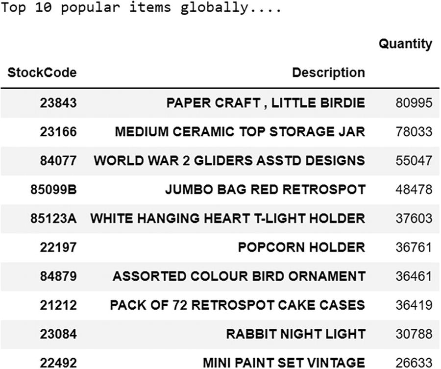
An output file depicts the top ten most popular items. It includes stock code, description, and quantity. paper craft, little birdie was the most bought item all over the region.

Let’s visualize it.

# vizualize top 10 most popular items

global_popularity.reset_index(inplace=True)

sns.barplot(y='Description', x='Quantity', data=global_popularity.head(10))

plt.title('Top 10 Most Popular Items Globally', fontsize=14)

plt.ylabel('Item')

Figure 1-11 shows the output of top 10 popular items.

A bar graph depicts items versus the quantity of the top ten most popular items globally. Papercraft, a little birdie has the highest range all over the region. medium ceramic top storage jar is the second highest item.

Popular Items by Country

Let’s calculate popular items by country.

# popular items by country

countrywise=df_new.pivot_table(index=['Country','StockCode','Description'], values='Quantity', aggfunc='sum').reset_index()

# vizualize top 10 most popular items in UK

sns.barplot(y='Description', x='Quantity', data=countrywise[countrywise['Country']=='United Kingdom'].sort_values(by='Quantity', ascending=False).head(10))

plt.title('Top 10 Most Popular Items in UK', fontsize=14)

plt.ylabel('Item')

Figure 1-12 shows that PAPER CRAFT, LITTLE BIRDIE is the most purchased item. It’s very popular only in the United Kingdom.

# vizualize top 10 most popular items in Netherlands

sns.barplot(y='Description', x='Quantity', data=countrywise[countrywise['Country']=='Netherlands'].sort_values(by='Quantity', ascending=False).head(10))

plt.title('Top 10 Most Popular Items in Netherlands', fontsize=14)

plt.ylabel('Item')

A bar graph depicts items versus the quantity of the top ten most popular items in U K. Papercraft, a little birdie has the maximum range with a quantity of 80000 approximately. Victorian glass hanging t-light has the minimum.

Figure 1-13 shows that RABBIT NIGHT LIGHT is the most purchased item. It’s very popular in the Netherlands.

A bar graph depicts items versus the quantity of the top ten most popular items in the Netherlands. Rabbit night light has a maximum range of 5000 quantities approximately. Space boy lunch box has the second highest range.

Buy Again

Now let’s discuss buy again. It’s another simple recommendation simple calculated at the customer/user level. You might have seen “Watch again” on streaming platforms. It’s the same concept. You know a certain set of actions are done repeatedly by a customer, and we recommend the same action next time.

This is very useful in online grocery platforms because customers come back and buy the same item again and again.

Let’s implement it.

# Lets create a function to get buy again output

from collections import Counter

def buy_again(customerid):

    # Fetching the items bought by the customer for provided customer id

    items_bought = df_new[df_new['CustomerID']==customerid].Description

    # Count and sort the repeated purchases

    bought_again = Counter(items_bought)

    # Convert counter to list for printing recommendations

    buy_again_list = list(bought_again)

    # Printing the recommendations

    print('Items you would like to buy again :')

    return(buy_again_list)

Let’s use the function on customer 17850.

buy_again(17850)

Figure 1-14 recommends the holder and the lantern to customer 17850, given that he often buys these items.

An output file depicts the often-bought items by customer 17850. The 21 items include a white hanging T-light holder and white metal lantern and more.

Summary

In this chapter, you learned about recommender systems—how they work, their applications, and the various implementation types. You also learned about implicit and explicit types and the differences between them. The chapter also explored market basket analysis (association rule mining), content-based and collaborative-based filtering, hybrid systems, ML clustering-based and classification-based methods, and deep learning and NLP-based recommender systems. Finally, you implemented simple recommender systems. Many other complex algorithms are explored in upcoming chapters.