How do we take into account the 3D nature of the earth when using 2D seismic data? Keep in mind our earlier contention that a 2D seismic section rarely represents a true planar slice through the earth. Furthermore, the interpretation of 3D workstation data is made through the collation of individual 2D profiles. The advantage of 3D data sets, as opposed to 2D data sets, is that the interpreter of 3D workstation data can select the location and direction of any 2D profile. Thus, the process used to aid in the construction of a valid interpretation is called “tying” the profiles together. Anyone who has worked with geophysicists has heard the phrases “tie the data,” or “tie the loop.” What tying the data does for the interpreter is build a 3D picture of the subsurface. Both structure contour maps and fault surface contour maps are 2D approximations of 3D geologic surfaces. It follows that two vertical sections intersecting a common surface (i.e., geologic log cross sections or seismic sections) will show the intersection of that surface at the same elevation on both profiles. This is illustrated in Fig. 5-11.

Figure 5-11. Intersection of seismic sections through a subsurface structure. Events must tie at line intersections because they represent the same subsurface point.

Even though this seems self-evident, the most common error in seismic interpretation is failure to ensure that all geologic surfaces that affect an interpretation have been tied around a loop along the lines. This includes tying the faults from line to line. For example, our experience with 2D and 3D data sets demonstrates that the failure to loop-tie fault surfaces can result in mapping two faults as one. The failure to loop-tie fault surfaces on 3D data can result in so-called trapping faults that do not exist. This problem is most important where, in the strike direction, one fault replaces another. This area is called the fault ramp or bridge (Chapter 11). The only cases where tying faults is difficult are in areas where the fault surfaces are near vertical, or in areas of complex deformation where the strike lines are poorly imaged. This may seem laborious (and often is), but the ability to tie surfaces by following a laterally continuous seismic event is one of the major advantages that seismic data has over well data. Well data forces the interpreter to infer a continuous surface from point information, whereas seismic data shows explicit continuity for the horizons and faults being mapped. By tying surfaces, you can eliminate some of the ambiguity that may arise when just using point information from well data. In effect, the act of tying both horizons and faults on a network of lines continually extends the surface and eliminates a number of possible surface configurations that may arise from the point data in wells.

Figure 5-12 is a set of diagrams illustrating the utility of tying surfaces in order to eliminate this three-dimensional ambiguity. Figure 5-12a is a fault surface map that was constructed solely from fault depth data derived from well log correlation. Figure 5-12b shows a different fault surface configuration that satisfies the same set of well log fault data. It is apparent that in some cases the point data from the wells are insufficient to uniquely define a geologic surface. An interpretation that satisfies the data may not be a unique solution. Figure 5-12c shows the same area with a set of two seismic lines, and Fig. 5-12d is a representation of these two lines, tied at their intersection and interpreted. To satisfy the requirement that all nonvertical surfaces should tie, it is easy to see that all but one of the possible fault surfaces cannot be justified with the grid of seismic data. Figure 5-12e shows a completed fault surface map, which is different than the other two but more accurate because both well data and seismic data are integrated into the fault surface interpretation.

Figure 5-12. (a) Possible interpretation of hypothetical fault data observed in a set of wells. (b) Another possible interpretation of the same fault data. Multiple fault surface interpretations are possible from this set of data. (c) Hypothetical seismic grid through faulted area. (d) Appearance of hypothetical seismic sections when interpreted and tied. Note that fault traces on profiles meet (tie) at the intersection of the two lines. (e) Final fault surface interpretation, integrating both seismic and well data.

Tying seismic data serves two important purposes. First, it establishes a relationship between the traces of surfaces seen on seismic profiles. In other words, by tying the data, we can assure ourselves that a given interpretation of a geologic surface on one line is indeed the same surface as interpreted on an intersecting line. This principle applies to both 2D and 3D data sets. The second benefit of tying seismic data is the ability to project the horizon being mapped into areas where well control may not exist. This forms the basis for many wildcat prospects. As previously mentioned, few wildcat prospects have wells near them. Seismic data allow you to extend a mapped horizon into areas with little subsurface control.

Do seismic interpretations have to tie between the grid of lines? The answer is a qualified yes. Ignoring 3D imaging problems for a moment, we can state that a valid interpretation must tie to be correct. All faults and horizons must be related and understood in the framework of a spatial grid of lines. The traces of geologic surfaces, as seen on seismic sections (the seismic events), must intersect at the tie points between lines.

Be aware of the tendency, however, to believe that a given interpretation must be correct because it ties between lines. Any nonvertical surface being interpreted on a section can be drawn to tie between any set of lines. Of course, when it is observed that seismic profiles show interpreted horizons crossing the actual seismic events, there is good cause not to believe in the interpretation. An exception occurs in reverse-faulted and thrust-faulted terranes where horizons may overlap because of faulting. More subtle problems can creep into the interpretation during the process of tying faults. Fault traces on seismic sections are sometimes difficult to see, and tying an array of closely spaced faults can present a near-impossible task, even on 3D data sets. An insufficiently spaced grid of seismic data in an area of dense faulting can present problems of aliasing, particularly if there is little data oriented along the strike of the faults. Figure 5-13 illustrates how aliasing can be a problem in highly faulted areas. Line Y is a strike line on which the faults are poorly imaged.

Figure 5-13. Ambiguity when tying closely spaced faults. Line Y is a strike line. Multiple interpretations may be possible.

The geometry of the faults in Fig. 5-13 may help with the tying problem. Notice that the maximum upper limits of two of the faults on line Z is the same as the maximum upper limits of the two faults on line X. It would be a reasonable first guess that the faults that die or are buried at the same elevation are the same pair of faults. This supposition, however, should be consistent with a believable tie and the construction of a reasonable set of fault surface maps.

Perhaps the most useful advice about tying data is to always think in terms of geologic surfaces and to regard what is seen on seismic sections as merely the trace of this surface intersecting the surface of the seismic line. Remember, however, that the time sections are not depth sections. Making geologic interpretations based on one seismic profile defies the 3D nature of the earth. Tying the data is a visualization tool that helps create a 3D representation of the subsurface.

Certain organizational procedures can save you unnecessary work during an interpretation. When you receive a set of paper seismic sections, it is tempting to immediately begin interpreting and mapping. A lot of unnecessary rework can be avoided by first taking the time to arrange the paper sections into stacks of data with similar orientations. For example, put all your north-south data into one pile, arranged consecutively from west to east or east to west. Similarly, put all your east-west oriented data into a separate pile, ordered consecutively going north to south or south to north. If your lines are arranged randomly, separate the lines into groups of roughly similar orientations. When you use a workstation, similar procedures can be conducted by scrolling through the 3D data set or by selecting parallel lines on the workstation.

Begin by selecting a line that is oriented in the same direction as the dip of the predominant geologic features you are interpreting. In areas of folds and thrusts, pick lines that are oriented perpendicular to the strike of the fold axes and thrust faults. In listric fault regions, choose lines oriented perpendicular to the strike of the listric faults, and so on. With each line, ask yourself questions about the structure. Which faults are the dominant faults? Where do the horizons show changes in apparent dip direction? Where are the crests of the highs and the bottoms of the lows? (Tearpock and Bischke 1991; see the section Long Wavelength Domain Mapping in Chapter 9.)

If using paper sections, unfold the next line and put it beside the first line. If at a workstation, bring up a new window and compare a new line to the existing line. Look at both lines and ask yourself more questions. Are the same faults present on this line as on the previous line? If a fault is almost certainly the same as one on the previous line, create a fault name, pick the fault, and, when using a computer, assign the picked faults to the same file. Do additional faults appear on this second line? If the dips change dramatically across the fault surface and the horizons lack compatibility, then the fault is likely to be large and will extend over large horizontal distances. Do the crests of the highs and bottoms of the lows change between the lines? Does the structural style change, or is it similar? Do the seismic dip rates at similar seismic times differ between the lines? What could be causing these differences? Pull up a third line and ask the same questions.

Continue this process of looking at two lines at a time until you have looked at all the similarly oriented lines. Make notes about major changes that you observe but cannot adequately explain at the moment. Now follow the same procedure with the strike lines. This may seem somewhat tedious and simple-minded, but we have found that a modest amount of time taken to do this sort of work is well worth the effort. It can save enormous amounts of time spent correcting mistakes made because you made too cursory an interpretation or became biased. We have found that when we are failing and having problems with an interpretation, doing this little exercise methodically and with a critical and questioning eye can help create an interpretation that is more likely to be correct.

We always peruse or scroll through a 3D data set before embarking on an interpretation. This procedure allows the interpreter to get acquainted with the structural style of an area and to get a better feel for and understanding of the data set.

Seismic profiles (e.g., Fig. 5-4) contain numerous reflections, and it is obvious that it would not be possible or practical to interpret and map every event. The interpreter should look critically at the sections and decide which seismic horizons are best to interpret and to map. Typically, the chosen events correspond to selected stratigraphic horizons, although reflection strength or continuity can also influence the decision.

Today, interpreters typically map sequence boundaries because not only are these boundaries commonly the most laterally continuous events on a section, but they are also directly related to rock type and the geologic history of an area. Sequence boundaries are geologic unconformities, or surfaces of erosion or nondeposition, and represent approximate isochronous surfaces (Payton 1977). They can generally be located on seismic sections by observing where reflections converge or are truncated against a (usually) strong event.

Sequence stratigraphic analysis is an exciting use of geology in geophysical interpretation. Covering this subject in any detail is a book in itself, and therefore we direct you to the references in the bibliography (in particular, Payton 1977; Berg and Woolverton 1985; Wilgus et al. 1988). You should be aware of the implications of this growing body of knowledge, as it has had and will continue to have a major impact on petroleum exploration.

Now that you are confident that your geologic interpretation is underway, mark the position of any wells that intersect the seismic lines. Straight holes require only that you have reasonably correct checkshot data close to the line. Directional wells require that a directional survey be available. Directional surveys and the projection of deviated wells into a seismic line are covered in Chapters 3 and 6. Remember that you must convert the depth points to their equivalent two-way travel times in order to annotate them correctly on a seismic section.

It is important to remember that any projection is a compromise and will commonly cause some confusion. Figure 5-14a is an illustration of a projection of a directional well onto a seismic section. Notice on Fig. 5-14a and b that an orthogonal projection of the well into the seismic line suggests that the well penetrated the footwall of the interpreted fault. However, the fault surface map (Fig. 5-14b) clearly shows that the well never crossed the fault from hanging wall to footwall; it is entirely within the downthrown block. This illusion occurs because of the compromises inherent in projecting a 3D entity onto a 2D profile. The routine orthogonal projection of a well into a seismic line can also cause significant mis-ties of horizons and faults.

(Seismic line published by permission of TGS/GECO.)

Figure 5-14a. Seismic section with directional well projected onto section (straight-line perpendicular projection used).

Figure 5-14b. Fault surface map of fault observed in Fig. 5-14a. Projection onto line makes well appear to have penetrated the upthrown block. Fault surface and the well’s directional survey clearly indicate that the well remained in the downthrown block. Care must be exercised in projecting wells onto seismic lines.

Once the well position is annotated, the information from the well data, in the form of geologic tops, must be located and marked on the time sections or loaded into the computer and annotated on the profile. How do you know where to find the event that corresponds to the geologic horizons? There are basically two methods used to tie the geologic control into the seismic data: (1) using a time–depth function calculated from checkshot data, or (2) tying into the seismic data with a synthetic seismogram.

The simplest but least accurate method of tying well data to seismic is to use the checkshot data to convert the tops from the log data from depth to time, and post the equivalent horizons on the seismic section at the proper times. The problem with this method is that you never know what kind of assumptions may have been made in the processing of the seismic line to correct to the proper datum. This is why data from different contractors may have static shifts between lines when tied together. “Ground truth” is hard to ascertain in these circumstances.

There is also a temptation to place unwarranted faith in the checkshot data and to believe it over all other information. We have seen cases where an interpreter tied a sand occurring in the middle of a 1000-ft shale interval to a level within a no-data zone and above a distinct event, simply because a nearby checkshot indicated such a tie. Particularly when sonic and density information indicate that a sand should generate a strong seismic response, it is likely that the sand ties to the strong event in the middle of the mostly reflection-free shale zone. This is not to say that shale intervals cannot generate strong seismic events. However, if a sand is present and fairly close to tying an event on the line, then correlate the sand to the reflection and don’t be misled by the checkshot listing.

Tying the well data into the seismic data with a synthetic seismogram is the preferred method, as it will usually provide reasonable results. Its usefulness, however, depends almost exclusively on the availability of good quality sonic and bulk density log data from the wells. In some areas, these logs are run as a matter of course, whereas in other regions they are the exception rather than the rule. Particularly in older basins, there may be a shortage of high quality sonic and density log data. It is imperative that the geoscientist determines the quality of the data used to make the synthetic seismogram. We have seen synthetics made from sonic logs obtained from washed-out wellbores that have recorded mostly mud arrivals and cycle skipping. Needless to say, the synthetic seismograms from such logs are useless.

Figure 5-15 shows a high-quality synthetic seismogram and its tie to a seismic profile. This seismogram is shown adjacent to a seismic section through the actual well location. As you can see, the match is good, though not perfect. The procedure for tying the proper event is to locate the chosen horizon on the log plotted next to the synthetic, then draw a horizontal line over to the synthetic trace. Lay the synthetic seismogram over the seismic profile at the appropriate location, then shift the synthetic up or down to determine if it matches the seismic data. The horizon line drawn earlier will show where the actual seismic event, corresponding to the log horizon, is located on the seismic line.

(From Badley 1985, provided by Merlin Profilers, Ltd.)

Figure 5-15. Tie of seismic data to synthetic seismogram. Events correlate well from synthetic seismogram to seismic profile.

Always be wary of forcing yourself to see correlations between the seismic data and the synthetic seismogram. If there are problems with either the seismic data or the synthetic data, it may be impossible to make a valid correlation. As a rule of thumb, a shift of the synthetic by more than about one hundred milliseconds should be highly suspect. Also, if you can turn the synthetic upside down and get equally good correlations, you should be suspicious of the validity of this method for tying well horizons into seismic data.

If applicable, this method of tying in the well data is preferable over tying into a particular seismic event with just checkshot data. If a correlation exists between the synthetic and the seismic profiles, then the synthetic seismogram method will ensure, with a reasonable degree of certainty, that the event being mapped is the intended geologic horizon. This is particularly valuable in areas of abrupt stratigraphic thinning and thickening. Figure 5-16 illustrates how an incorrect pick for the mapping horizon can have a profound effect on the depth of the horizon away from the well control. As shown, a small error in the thinner stratigraphic section will cause a much larger error to occur where the stratigraphic section is thicker.

Figure 5-16. Increase in magnitude of error in areas with rapid changes in interval thicknesses. Any uncertainty in tying formation top to seismic event can introduce a greater uncertainty where stratigraphic section thickens away from well control.

A vertical seismic profile (usually abbreviated VSP) derived from a synthetic trace is also an excellent tool for tying into the seismic data. The methods for using the VSP to tie into the seismic line are the same as those used for synthetic seismograms. Establish a correlation between the traces on the VSP and the seismic, and use the plotted log as a guide for tying into the seismic section. An added benefit to both the synthetic seismogram and the vertical seismic profile is the ability to use these data to analyze the relationship between the lithology in the well and the seismic character.

The subject of tying well information into seismic data is deceptively simple. There is a dangerous tendency to believe that your first tie from a well is the correct one. Make sure that it is, because being tied into the wrong horizon can cause you to miss the relationship between a given log response and its correlative seismic response. The only other advice we can give is to avoid a “railroad track” mentality (looking strictly at a narrow 80-millisecond strip of the seismic data), or you may totally miss what is present above and below the horizon you are mapping.

We strongly recommend that fault surfaces be loop-tied prior to loop-tying horizons. Geophysicists loop-tie surfaces for the same reasons that geologists loop-tie stratigraphic markers. That is to make sure that you are on the same surface where you began, and not on a different surface. Mapping faults first has distinct advantages. First, in areas of complex structure the style of faulting helps determine the type of structures that exist in the area (Chapter 10). How can you determine how the structure formed if you do not understand how the faults behave in three dimensions? Second, problems may arise when mapping horizons on portions of a profile that contain a lower seismic frequency or where the data are not perfectly coherent. If the position of recognized faults has not been identified in three dimensions, then geoscientists may map horizons right through fault surfaces. This will result in a horizon mis-tie, as described in the next section. Our examination of the horizon mis-tie problem on many data sets indicates that the geoscientist may not even suspect that an existing fault produced the mis-tie. After all, the assumption was made that the faulting is understood or that fault surface mapping is not required. The result is that the geoscientist may create a nonexistent fault to solve the mis-tie problem. The nonexistent fault constructed through semicoherent data or data that abruptly changes reflection character creates additional mis-ties and more nonexistent faults and mis-picked horizons. We have seen cases where prospects have been generated as a result of the nonexistent faults. Needless to say, the wells were dry.

There is another common problem with the picking of nonexistent faults in semicoherent data or data that rapidly changes reflection character. These nonexistent faults may actually be axial surfaces or changes in bed dip that are common to compressional and salt-related folds (Chapter 10). Where the geoscientist encounters a nonexistent fault, the horizons must be offset, which results in a horizon mis-pick. A mis-picked horizon results in mis-ties and in other nonexistent faults that are created to solve the mis-tie problem.

However, if fault surface maps are constructed for each of these nonexistent faults, the fault may not map as a smooth curved surface, but will contain offsets and kinks. The presence of an offset or kink typically implies more than one fault. Also, the overall geometry of a mapped fault surface may be simply unreasonable. These types of fault surfaces are not viable geologic surfaces and should be rejected. Faults that map as smooth surfaces are considered more plausible. Furthermore, with 2D data sets, questions typically arise as to which faults link to form a continuous fault surface. Fault surface maps can help resolve the fault correlation problem.

We find that mapping fault surfaces not only results in better interpretations and in higher quality prospects, but the process saves time. The time taken to construct quality fault surface maps is justified when you consider the time required to attempt to solve existent and nonexistent mis-tie problems, the reworking of an interpretation that proves incorrect, and the costs of an unnecessary dry hole.

If you have followed the procedures so far, you now have a tentative interpretation and well data annotated on each profile. To this point, we have not described loop-tying the data. That is the next step. On a good day, portions of your preliminary interpretation will probably be wrong when you finish loop-tying the data. Again, methodically tying the loops will improve the chances of finishing the task correctly and in a timely manner. The use of a workstation has advantages in that any errors encountered during the interpretation can be readily corrected and alternative ideas can be easily tested.

We find it much easier to interpret the most obvious geologic features first and to tie them together on all the lines. After the large features tie, begin another iteration of tying through the data volume, concentrating on the smaller “second order” features. As the size of the features being tied together decreases, the number of lines required to tie them also decreases, so the work goes more quickly toward the end of the process.

It is important to pick a loop-tying scheme that will allow you to make the smallest number of assumptions while carrying your surface around the map area. Tying a path that crosses the fewest faults and that crosses faults at their location of smallest displacement will more likely be correct.

The initial task for tying the loops is to post all the intersections of the seismic data on all the lines. With paper sections, depending on the number of lines that are being tied, this process can take anywhere from a morning to several weeks. Figure 5-17 shows a seismic base map with two seismic lines. The corresponding profiles are shown in Figs. 5-18 and 5-19. Line A intersects line B at a location just north of shotpoint 480 on line B.

Figure 5-17. Seismic basemap showing positions of seismic lines A and B.

(Seismic data published by permission of TGS/GECO.)

Figure 5-18. Seismic line A. Profile shows gently dipping reflectors cut by a small growth fault.

(Seismic data published by permission of TGS/GECO.)

Figure 5-19. Seismic line B. Profile shows gently dipping reflectors cut by a small growth fault.

Line intersections are seldom cooperative enough to fall on a downline (a downline, shown in Fig. 5-7, merely refers to the dark vertical line printed on the time section at the shotpoint locations annotated on the maps). Depending on the precision required, you can either make a rough estimate of the intersection or use a scale to determine that the intersection is exactly 150 ft, or 1.829 traces to the right of shotpoint 480 on line B. All the intersections that you intend to tie together must be marked.

The next step, when using paper sections, is to fold one of the lines at the marked intersection. This fold must be vertical. Use a straightedge to ensure that the section is folded vertically. Align the folded section with the unfolded section at the appropriate intersection. Figure 5-20 demonstrates a tie between the two paper sections. On the workstation, the horizon intersection picks are posted automatically.

(Seismic data published by permission of TGS/GECO.)

Figure 5-20. Seismic lines A and B intersected with each other. Notice line A appears to be too “shallow” in relation to line B when the timing lines are aligned.

Figure 5-21. Keeping track of relative mis-tie through a grid of seismic data. All absolute mis-ties are in reference to reference line.

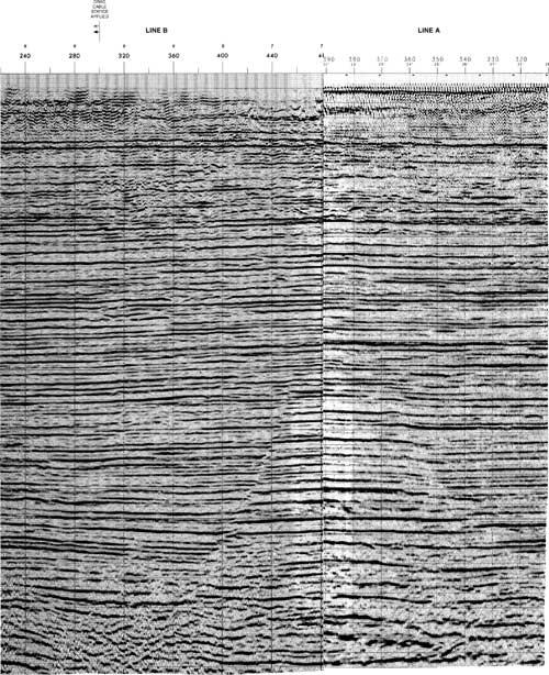
The first thing you will probably notice is that the lines may not tie perfectly when the intersecting lines are aligned at a common two-way time (Fig. 5-20). Sometimes they will match perfectly, but more likely, they will not match at a common time. At least one section will have to be slightly shifted vertically to establish a good correlation between the lines. Figure 5-21 shows how the two lines have to be shifted relative to one another to “tie” the events. Which line has been shifted? Has line A been shifted down 10 milliseconds (+ 10 ms), or has line B been shifted up 10 milliseconds (− 10 ms)? You now decide which line shows the “real” two-way time to the event.

In an interpretation and mapping project of any complexity, it is necessary to pick a reference seismic line so that all the other data may be posted with the appropriate time shifts relative to the reference line. In effect, the procedure for choosing a proper reference line is similar to that for picking a correlation type log (Chapter 4). When using wells, you are picking the log that best demonstrates the geologic section of the mapping area. When choosing a reference line, pick a line that has as many of the following characteristics as possible.

Static mis-ties can be recognized because they cause “bulk” shifts of the intersecting line, either up or down to achieve a good correlation (Sheriff 1973). They commonly occur between data sets of varying vintages and contractors because of different datum corrections and assumptions. Figure 5-20 shows a static mis-tie between two intersecting lines. The easiest way to determine a static mis-tie problem is to search for any shift between flat-lying events that are normally present in the shallow part of most basins. In Fig. 5-20, line A ties line B perfectly with a static shift. We do not know, however, if the times on line A are too large or if the times on line B are too small. There is no absolute answer. This is the reason for picking a reference line; it establishes a reference or datum. The rest of the lines can then have the time picks for a given event adjusted to the datum established by the reference line. If a line does not directly intersect the reference line, then its relative mis-tie with a line that does intersect the reference line is added together with the adjustment value from the line intersecting the reference line. This is harder to describe than to illustrate, so Fig. 5-21 shows an example for keeping track of static mis-ties on lines that do not directly intersect the reference line.

Once a reference line is chosen, annotate the rest of the sections with their respective static mis-tie values relative to the chosen datum. An important point to note about this process is that it should be carried out only where you are tying events that are relatively low-dip (probably less than 8-10 deg at most). High dip rates cause an effect called migration mis-tie, which is discussed next.

A migration mis-tie is one of the more difficult aspects of interpretation of 2D seismic data, and it becomes problematic in areas of high bed dips. As noted previously, you may encounter varying amounts of mis-tie with different time ranges of events. In general, the shallow, low-dip events will tie reasonably well with a static shift. But as the dip increases with increasing depth (greater time on the section), you may notice that events on the dip lines appear to be too deep (too large a time) relative to the intersecting strike line. Figure 5-22 is a sketch of this phenomenon. This mis-tie problem is present because of the limits of 2D seismic data in imaging a 3D surface.

Figure 5-22. Appearance of migrated strike and dip lines at their intersection. Notice events on strike line are too “high” (too small a time).

To understand this problem, it is first important that you understand what the migration process does to seismic data. Figure 5-23 is a simplified illustration of a 2D seismic line shot in the dip direction. Two simple, normal incidence raypaths are drawn on the section from surface positions A and B. By definition, a normal incidence ray will intersect the reflector Z at a right angle. Raypaths drawn to satisfy this condition are A-A′ and B-B′. Assume the two-way travel time for a reflection from point A′ is 2.0 sec and the two-way travel time for a reflection from point B′ is 2.1 sec. Both these reflection points are being recorded at the surface at positions A and B, respectively. So, on an unmigrated seismic section, the events appear to have the positions shown by dashed line Z′. The seismic lines are recording data at surface locations A and B from subsurface reflection points A′ and B′, which are located up-dip of surface locations A and B.

Figure 5-23. Diagram illustrating why data need to be migrated. Subsurface reflection points A′ and B′ are positioned at A″ and B″ on unmigrated data. Migration moves points A″ and B″ back to their actual time positions A′ and B′.

Migration is a fairly complex process that corrects the data by moving it back to its proper time position relative to the surface location. In other words, after migration, a reflection point should be positioned correctly with respect to the surface recording points. Migrating the example would move the event Z′ to a position coincident with the actual event Z. Migration will always steepen events or reflectors and cause a given event to appear “deeper” (occur at a larger time) for any given shotpoint when compared to the unmigrated data. Migration of the seismic time data is critically important in obtaining a reasonably accurate interpretation of the subsurface.

The problem with migration is that it can fully correct only a true dip line. Because the 2D migration algorithm cannot move data from out of the plane of the line, a line that has an apparent dip and not true dip will not be fully corrected. Figure 5-24 shows the extreme case: a true strike line that is oriented perpendicular to dip direction and thus contains no component of dip whatsoever. The data are still being recorded from up-dip, but the migration algorithm cannot move data out of the 2D plane of the line. The apparent dip is zero, so the migration algorithm really has no effect on the line. Event Z is positioned on the line at the two-way time of A-A′ and B-B′, much shallower (smaller two-way time) than is really the case beneath the surface line A-B. Figure 5-22 shows what occurs at the intersection of a true dip and true strike line. All the events on the strike line appear to come in too shallow (too small a time). This is important to remember when tying data. Only in very peculiar circumstances will a strike line event intersect a dip line deeper (greater time) than the corresponding event on the dip line. (This assumes that any static mis-tie has already been taken into account.)

Figure 5-24. Strike line imaging. Reflection path for strike line is not underneath the line. Data is being recorded from up-dip.

Figure 5-25 illustrates what effect a migration mis-tie can have on a line intersection in areas where there is increasing dip with depth: The mis-tie becomes larger and larger in the deeper (greater time) part of the section. In an interesting twist to this problem, notice that the strong event at about 2.6 sec on the strike line is actually “deeper” than its correlative event on the dip line. How can this be possible if the data are coming from up-dip? Notice that all the events are too shallow on the strike line until about 2.4 sec, when they begin to appear deeper. By tracing horizontally (isotime) from the strike line to the dip line, we can see that the events are deeper because they are being recorded from up-dip, which happens to be downthrown to a buried growth fault, whereas the section ties the dip line in the upthrown block. Notice also that the fault intersection point on the strike line is actually 300 ms deeper than a “mechanical” tie would indicate. In growth fault areas, this problem is not uncommon. Many growth faults have larger dips in the nongrowth sediments located beneath the fault at depth.

(Seismic lines published by permission of TGS/GECO.)

Figure 5-25. An unusual case of migration mis-tie. Strike section events occur earlier (“shallower”) than same events on dip section until approximately 2.4 sec. At the bold event at 2.6 sec, strike line continues to record up-dip; however, this is also downthrown to an expanding growth fault.

The problem can be handled in two ways. The first and easiest method is to use the strike lines only to tie the events among the dip lines, but ignore them as valid sources of data points for drawing maps. In areas where there is already abundant well control and adequate density of dip-line coverage, this may be a viable option. The strike lines can still be used to tie events among the lines, but their actual time values are ignored. The disadvantage of this method is that the strike lines contain information on cross structures that is often critical to development of a potential hydrocarbon trap (see Chapter 11).

The best option (and the most time consuming) is to explicitly correct the strike line data by moving the data to their proper position relative to the surface locations. There is an easy graphical way to accomplish this task that the 2D seismic workstation does not automatically provide. Figure 5-26a shows hypothetical dip and strike lines posted on a structure map. Figure 5-26b shows an intersection of migrated lines A and B, as they would appear on migrated time sections. If you assume that the dip line A is properly migrated, then the data on strike line B at the intersection is actually coming from a position that is up-dip of the intersection with the dip line.

Figure 5-26. (a) Approximate method for dealing with migration mis-tie involves relocating strike line data points up-dip as determined from a true dip line. (b) Method for calculating the distance that strike data must be moved to account for migration mis-tie. Find intersection of time observed on strike line (at line intersection) with the same event on dip line.

This concept is easier to illustrate than to explain, so Fig. 5-26b shows an imaginary horizontal line drawn from the event intersection on the strike line to its real reflection point on the dip line. The process for correcting a series of lines is to find the actual reflection points for all the intersections of the strike lines with dip lines, and to mark these points on the map. These points locate positions near where the reflected event actually originated (Point A on Fig. 5-26b). If this procedure is carried out over a series of intersections, then a “corrected” base map can be made that shows the approximate reflection path of the strike line. The dashed shotpoint display in Fig. 5-26a illustrates how to “relocate” the strike line up-dip before posting the data points to use in making a map. Once this corrected base map is made, interpolate the individual shotpoints and post the times from the strike lines at their approximate subsurface locations. One important point about this technique: Any correction is only valid for the particular event being interpreted and loop-tied. For example, another event that is deeper may require another corrected base map to be constructed for its structure map. In other words, the correction is not a fixed value, but rather, varies depending on the depth of the event being mapped.

This discussion has been directed toward tying actual seismic events among lines. Faults must also be tied, and in areas with high bed dips, the migration mis-tie problem can make mapping fault surfaces extremely difficult. It is vital to remember that if the fault surface reflections are coming from somewhere other than beneath the line, then the fault surface reflection is subject to migration effects. What makes mapping faults especially difficult is the spatial aspect of the migration mis-tie problem. It is entirely possible to have data points for a given fault surface coming from further and further away from the line, simply because the profile crosses the fault at an oblique angle. This causes the fault to change depth relative to the profile. Figure 5-27a shows two seismic lines that intersect each other. Line A is a dip line and shows increasing dip of the seismic events with increasing time (depth). Line B is a strike line with an obvious fault cutting the events on the line. It is obvious from the tie that the events on line B are actually coming from up-dip of the surface location of the line. The discontinuity in the events is caused by fault X, and thus the image of fault X is also coming from up-dip of the surface location of the line. Point “X” on Line A in Fig. 5-27a is the actual tie point for fault X. Figure 5-27b is an illustration of the method used to construct a corrected fault surface map by moving the times for the fault trace further and further up-dip with increasing depth of the fault. The complex nature of the migration process illustrates the advantages of 3D migration.

Figure 5-27. (a) Hypothetical dip and strike lines with fault observed on strike line. Notice the effect that an increasing amount of dip, with increasing depth on the dip line, has on the correlative events on the strike line. (b) Relocation of fault surface points to proper spatial location, using method outlined in text. Notice that the change in the distance the points must be shifted actually changes as the record time (depth) increases.

When interpreting by hand, the most obvious type of data to post from seismic sections are the actual two-way travel times for the events that correspond to the geologic horizons being mapped. This is analogous to posting formation tops on the map when using well data. The same two-way travel times can be posted for any fault surfaces being mapped. There are several other types of mapping information that can be extracted from the seismic data. One type of information that is extremely useful is the upthrown and downthrown intersections (cutout points) of the horizon being mapped with the surface of a fault. These intersection points have both a vertical datum and a location associated with them. The significance of these points, assuming the data is reasonably high quality, is that they can be used to help position the upthrown and downthrown traces of the fault and the approximate width of the fault gap. In practice, seismic methods overstate gap width by about a factor of 2, and the correct width of the gap is finally derived from structural horizon and fault surface map integration (Chapter 8).

Many interpreters post a solid bar on the map in an easily identifiable color to indicate the fault trace identification. In complex areas, you can assign a unique color code to each fault being tied on the seismic sections and post the trace on a base map in the same color.

Depending on the area, there may be some other useful information that can be posted on the map. If the seismic event being mapped has an amplitude anomaly associated with a hydrocarbon-bearing sand, then the areal extent of the amplitude anomaly can be posted. In areas adjacent to salt domes, you may be fortunate to have data sufficient to identify a salt/sediment interface. This contact can be posted and mapped. In areas with stratigraphic discontinuity in the objective sands, you may be able to detect a unique seismic response indicating where the sand is present and where it is not. The extent of the potential reservoir body can thus be mapped.

When tying the data around a loop by hand, use a colored pencil to color in the troughs of the seismic data. At each downline or shotpoint marked on the line, mark with a pencil a consistent part of the waveform, using either the maximum trough (which is easy to see), the maximum peak, or the crossover.

Now that the data have been interpreted, they have to be transferred from the seismic lines to the base map. With an engineer’s scale, measure the two-way time in milliseconds to the event being mapped. Next, add or subtract the constant value in milliseconds that represents the amount of static mis-tie between this seismic line and the reference seismic line. Post the two-way time on the map at the actual reflection point for the horizon being mapped. If you constructed “pseudo” base maps with all the strike lines repositioned up-dip, post two-way times at the “corrected” shotpoint locations. Remember that the adjusted strike line location may vary, depending on the depth of the seismic event that is being mapped. Mark all the intersections of the seismic events associated with fault surfaces, and post the upthrown and downthrown intersection (cutout) points. Finally, record any other valuable information and post it on the map.

The first method for converting time to depth is extremely easy. The procedure for converting the values involves determining the depth values corresponding to the posted time values in a time–depth table that has been generated from checkshot data. Checkshot data is acquired during the evaluation phase of drilling a well. A checkshot measures the amount of time it takes for the first arrival of a seismic wave to travel from a surface source near the well to a receiver lowered down the wellbore. After the data are acquired, they are usually interpreted to generate a set of one-way travel times for specific depths in the well.

Conversion of these one-way times to two-way times involves multiplying the time values by two. (The receiver only measures the time it takes for a wave to travel to a given depth, whereas a seismic line measures the time required for a wave to travel to a reflecting horizon and back to the surface.) The two-way time–depth pairs are then interpolated from the usually sparse set of data points to generate a table with the time–depth pairs calculated at even increments of time. Such a table was shown in Fig. 5-8. A plot of a particular checkshot can be shown graphically by constructing a time versus depth graph. The actual times are shown as data points, and a line is fitted to the data points using a cubic spline curve-fitting computer program.

Once the correct depth for a given two-way travel time has been found, you can post the depth value beside the time value on the map. Using a contrasting color pencil to post depth information is a good method for keeping the time values distinct from the depth values you will use to contour the map.

Where should this method be used? Use this simple technique in areas where there does not appear to be any large lateral variations in the relationship between seismic time and depth. The method for determining whether this is appropriate is as follows. First, use a time–depth table generated from the closest well to the mapping area (or a well in the middle of the area) to convert all the times to depth. Second, examine your map, looking for obvious discrepancies between the well tops posted on your map and the converted time values. If, for example, the depth from a converted time value is 11,200 ft subsea, and a well top at the same location is 10,700 ft subsea, then there is an obvious problem to be addressed.

If the velocity information does not tie accurately to the wells, there are two possible sources for the differences in the values posted. One possibility, often overlooked, is that the wrong horizon was interpreted on the seismic line, and thus inappropriate time values are being converted to depth. This problem could arise from an incorrect pick across a fault or from an incorrect tie to a well. The error can be caused by using too large a shift to tie to a synthetic seismogram. Perhaps the synthetic seismogram contains problems related to log quality or some other factor. There exists a whole multitude of possible causes similar to these.

Another possibility is that there is a strong horizontal velocity gradient in the area that causes the time–depth relationship to change laterally. Lateral variations are often easy to determine if you have logs and synthetic seismic events that are easy to correlate in two wells. In this case you absolutely know that both the correlations and time picks on seismic data are correct and the correlations in the wells are correct. However, the correlations between the wells don’t agree with one another. In other cases, the problem may not be so easy to identify. If either the well correlations or the seismic event ties are ambiguous, the presence of a gradient may not be obvious because of the difficulty in deciding what interpretation to rely on initially.

Lateral velocity changes can be extremely difficult to manage. It is beyond the scope of this book to attempt a complete discussion of the methods of handling velocity gradients. The key question is when to recognize the need for expert help. A simple rule of thumb is this: If the gradient in the area being mapped is severe enough to cause the depth uncertainty for a given two-way time value to exceed the average amount of closure on the features you are mapping, you should be careful. In particular, if this depth uncertainty can be observed to occur between check shots in wells that are as physically close as the average dimensions of a prospective closure, the likelihood of correctly mapping a structural closure is small. If a problem exists, seek the assistance of a senior geophysicist who understands all aspects of handling velocity gradients.

If the magnitude of velocity changes over your mapped area is not severe, you can often “eyeball correct” a map to account for a gradient. To correct for gentle gradients, interpreters may make ad hoc adjustments to the map to account for the horizontal velocity gradients. In practice, interpreters will attempt to find the geologic reason for the velocity differences and use a different time–depth table on either side of the geological “boundary” causing the anomaly. For example, in the Gulf Coast tertiary section, a large growth fault will commonly have downthrown section that has a different velocity field than the upthrown section. In some areas, the seismic velocities may be faster on the downthrown side because of the increased amount of sand in the downthrown block. In other cases, the seismic velocities may be slower in the downthrown block because the thickened section was deposited rapidly and is undercompacted and slightly overpressured, and therefore the velocities are slower. Whatever the situation, if you can determine the reason for the gradient, you can often adjust the contours to honor the well control.

We have found that the easiest way to handle velocity gradients that do not appear to have definite “boundaries” is to use the following technique, illustrated in Figs. 5-28a-d. A base map with posted information obtained from both well logs and seismic sections is shown in Fig. 5-28a.

Figure 5-28. (a) Base map showing posted seismic two-way times and formation tops from well data for a mapping horizon. (b) Isotime map of seismic two-way data. (c) Preliminary depth map constructed from each point of control. Contouring begins at each point of well control and moves outward. (d) Final depth map with horizontal velocity gradient “lost” in the syncline between the two plunging noses. The difference in depth values has been adjusted in the contouring of the syncline between the well control points.

First, prepare a pure-time map. Map the isotime contours of the time values, as shown in Fig. 5-28b. Next, determine the average velocity in the depth range being mapped. Simply determine the number of milliseconds of two-way time that the contour interval, in depth, represents at the depth range you are mapping. A typical Tertiary value might be about 22 ms per 100 ft. At each point of well control, use the time map as a guide and begin contouring in depth, using the distance between each time contour as a rough indicator of the magnitude of bed dip. Carry the contours about halfway to the next well and then start at that well and contour away from that well until you meet the previous contours (Fig. 5-28c). The discrepancy in the depth values can then be adjusted by splitting the difference between the two sets of contours and gradually adjusting the mis-tie in the spacing of the depth contours (Fig. 5-28d).

The points to remember about this technique are, (1) it is quick but imprecise, (2) it is appropriate when applied to minor velocity problems over large areas, and (3) it is useful when the map must be finished quickly. A caveat: Never use this technique when the gradient is severe and is present over a single structure. It is an appropriate and useful technique when you are mapping on a large scale and need a method of “absorbing” the mis-ties in the synclines between the major closures. Remember that seismic data do not have the vertical resolution of well data. A seismic line sampled at 4 ms and picked to an accuracy of 10 ms will give you about 40 to 60 ft of error in an average Gulf of Mexico Tertiary section. Using this technique to account for a 200-ft mis-tie problem seems acceptable.

The most important point to remember about velocity problems is that it is very easy to exceed your expertise with simplistic solutions. Look critically at your data and get assistance if it is needed.