
The first edition of ASGM contained one chapter on structural geologic methods. Since knowledge of structural geology plays a key role in interpretation and mapping, as discussed in number 2 of the Philosophical Doctrine, we believed the chapter was important to the overall content of the textbook. Because of advances in structural geology and balancing during the past decade, in this second edition we have expanded the one chapter into four separate chapters covering compressional, extensional, strike-slip and growth structures. Knowledge of structural methods in these various tectonic settings will improve your ability to generate viable, three-dimensionally valid interpretations, maps and prospects, as well as improve your ability to develop field discoveries.
We begin the structural geology section of the textbook with a review of compressional techniques and methods. Much of modern structural geologic analysis began with the study of compressional tectonics, and therefore it is appropriate to start here. These four structural chapters center around specific structural methods and techniques. A basic understanding of rock mechanics, structural geology, and balancing, presented in such textbooks as Billings (1972), Suppe (1985), Woodward, Boyer, and Suppe (1985), Marshak and Mitra (1988), is a prerequisite to understanding and applying the techniques presented in this chapter.
Compressional structures contain extensive proven petroleum reserves in many areas of the world. But even more accumulations remain undiscovered, and existing fields are insufficiently exploited, because the typical complexity of compressional structures and inadequate seismic resolution inhibit reasonable and accurate interpretation and mapping. Critical to the best possible analysis of the data is the interpreter’s knowledge of compressional structural geology and the application of techniques that lead to geologically reasonable interpretations and accurate maps.
One of the most important of the compressional structural geologic techniques is structural balancing. The ultimate goals of balancing are to restore complexly deformed rock to its initial state or to its correct palinspastic restoration and to determine the geologic sequence of events. Such information can be very useful to the geologist or geophysicist. Not only is the geometry of the structure better understood, resulting in better and more accurate prospect and reservoir maps, but geologic trends such as sand patterns can be more accurately located. An understanding of the timing of the structural events should aid in oil migration studies and define how and where fluids may have entered the structure. If the geometry of the structure is understood, then this knowledge can be used to more accurately process seismic data, which in turn results in an even better understanding of the geometries. Balancing can also be effectively used to check assumptions and interpretations (Tearpock et al. 1994). Lastly, balancing tends to keep the interpreter more focused. If the section does not balance, then perhaps it is time to reconsider the interpretation. Why drill a well to determine that the interpretation does not balance when restoration can determine a misinterpretation prior to the drilling? Our experience with balancing, as well as that of our colleagues, indicates that balanced, geologically possible interpretations can discover significant additional reserves. In short, balancing works.
Structural balancing is based on the intuitively satisfying concept that the interpreter must neither create nor destroy volume during the interpretation process (Goguel 1962). Interpreters may inadvertently introduce a volume imbalance anytime a fault is mis-picked or a horizon is miscorrelated. Fortunately, balancing can detect volume problems prior to the drill bit. Thus, it follows that an interpreted map or cross section, whether it be a geologic or seismic section, should volumetrically restore without overlaps or voids in the stratigraphic section. Faulted and folded beds should be restorable to their initial subhorizontal state (Tearpock et al. 1994). Thereby, a structural interpretation may be tested for admissibility. An analogy might be a child who removes a new block puzzle from a box and places it on the floor. Once all the pieces of the puzzle have been removed from its container, the puzzle can be restored to its initial state by placing each block back into its proper position. The first attempt by the child at restoring the puzzle may result in most of the pieces being placed into the box, with one or two pieces remaining on the floor. A second attempt could result in all of the pieces being placed in the box, but with some of the pieces being tilted at various angles or forced to fit.
The geoscientist experiences similar problems when attempting to retrodeform (restore) geologic and/or geophysical data. Of course, the correct solution to a puzzle is one that has been perfectly restored to its initial position. There are two types of interpretations: interpretations that are admissible, or geologically possible, and interpretations that are inadmissible, or not geologically possible (Elliot 1983). A balanced interpretation is an admissible interpretation in which the horizons can be restored to their initial subhorizontal position by unfolding the horizons and rotating the beds back to a subhorizontal position along the interpreted faults.
The benefits of balancing are fundamental to correct geologic interpretations. The earth’s subsurface contains no voids or mass overlaps; thus, a section that does not balance cannot be geologically reasonable on simple geometric grounds. Unfortunately, a balanced section, although physically reasonable, need not necessarily result in the correct geologic interpretation. Balancing is not unique, and two geoscientists can produce two balanced sections that are not alike. Obviously, the more complete the data set and the better the interpretive techniques, the more likely that the balanced section will reflect reality.
Balancing is still a developing science, and new techniques and interpretations are progressively being introduced. Nevertheless, an interpretation tempered by a concept of mass conservation is the key to admissible geologic interpretations and constructions. If the structural interpretation is correct, then balancing techniques can be used to quantify the interpretation.
Balancing can be subdivided into two disciplines: classical balancing, which was primarily developed by Goguel (1962), Bally et al. (1966), and Dahlstrom (1969) and his coworkers, and nonclassical balancing, which was primarily developed by Suppe (1983, 1985) and his students and coworkers. Most of the concepts presented in this introduction can be attributed to Goguel and Dahlstrom.
For many years, structural geologists have argued about the mechanical properties of the upper crust. Does it exhibit elastic and/or frictional behavior as indicated by earthquakes, or is it viscoelastic or viscoplastic, as indicated by the bent strata in the hinge zone of folds? Could time be a factor? Do the sedimentary strata buckle out (Biot 1961), or do the strata follow faults within the sedimentary section (Rich 1934)? Although all of these mechanisms are possible, the evidence now strongly suggests that the deformation that occurs in petroleum basins is primarily controlled by brittle (low temperature) deformation processes, and that the viscous deformation expressed by fold trains (Fig. 10-1) is confined to metamorphic belts (Tearpock and Bischke 1980). The fold style depicted in Fig. 10-1, with its near constant wavelength, is not commonly observed in petroleum basins, and thus another deformation mechanism is required to explain the folds that trap hydrocarbons. This mechanism appears to be frictional deformation. Davis et al. (1983), Dahlen et al. (1984), and Dahlen and Suppe (1988) formulate a frictional, or brittle, theory of crystal deformation that applies to both compressional and extensional regimes. The theory resolves the overthrust paradox (Smoluchowski 1909; Hubbert and Rubey 1959) and is consistent with the geologic and seismic information collected from petroleum basins. Our intention here is to apply this theory and its observations to our areas of interest. Those readers who maintain an interest in mechanics can consult the references listed at the end of this textbook.

The frictional theory of crystal deformation states that when folds form, the maximum principal stress (σ1) is inclined slightly to the bedding surfaces (Fig. 10-2). The rock will then fracture along angles that are dependent on the pore pressure and the intrinsic strength of the rock. The weaker the rock, the lower the angle between σ1 and the fracture.

For example, consider an alternating sequence of limestone and shale layers (Fig. 10-2). Intuitively, shale layers seem to be weaker than better consolidated limestone layers, and it is well known that shales can contain abnormally high fluid pressures that drastically weaken these rocks. The theory states that because shales are weaker than limestone, the angle (α1) between σ1 and the fractures in shales must be smaller than the angle (α2) between σ1 and the fractures in limestones (Fig. 10-2). As σ1 is slightly inclined to the bedding, the fractures in the shales are more subhorizontal than the fractures in the limestones. This leads to the primary conclusion of this section: In more competent or stronger rocks, the fractures will form at a high angle to bedding, and in the incompetent rocks, such as overpressured shales, the fractures tend to form parallel or subparallel to bedding.
If motion along these fractures causes them to coalesce, then a decollement, or zone of detachment, will form along the flat-lying bedding and may follow incompetent (shale or evaporite) horizons for tens or even hundreds of kilometers (Davis and Engelder 1985). In areas where the weaker layers gain strength or are pinched or faulted out, the decollement may ramp to a higher structural level (Fig. 10-2). As these ramps must pass through rocks that are stronger and have lower pore pressures than shales, the angle (α2) between σ1 and the fractures will be larger. Thus, ramps have higher angles with respect to the bedding than do the flatter portions of thrust faults (Fig. 10-2).
Where the ramp connects to a weaker layer on a higher structural level, the ramp transforms into a flat once again. Once a network of ramps and flats form and a large force is applied to the back of the wedge-shaped region in Fig. 10-2, the strata above the flats and ramps will begin to move along the fault. Material will begin to slide along the flats and up the ramps, forming a fold in the hanging wall block. Eventually, large folds will form in a manner that was initially described by Rich (1934), but this process is the subject of a later section.
The angle at which the ramp steps up from the bedding is called the cutoff, or step-up, angle (θ in Fig. 10-2). This angle is often characteristic, or fundamental, to a particular fold-thrust belt and depends on both the pore pressure in the rock and the rock type. Similar relationships may exist in extensional terrains. The characteristic cutoff angle in certain fold-thrust belts is generally less than 20 deg and tends to vary within several degrees of its mean value. For example, in Taiwan the characteristic step-up angle is 13.3 deg +/– 2.4 deg (Suppe and Namson 1979; Dahlen et al. 1984). An attempt must be made to determine this angle prior to a balancing study. This step-up angle will be used to balance your structures. Note that the step-up angle is measured relative to regional dip rather than to the horizontal.
There appear to be at least three methods which give insight into estimating the characteristic step-up angle. Field studies or a literature search can be conducted in the area of interest. As the step-up angle is the angle between the flat and the ramp, field measurements or a description of this relationship will provide the required answer. A second, less direct measurement technique is to observe a well-imaged ramp and flat on a seismic section that is perpendicular to the strike of the fault surface. The section must first be depth-converted to make this measurement. The strata above the ramp will parallel the ramp, and thereby the step-up angle can be determined relative to regional dip (Fig. 10-33). Therefore, a study of the dips across an area may give insight into the characteristic step-up angle. For this method, it is first necessary to know the regional or undeformed dip of the area. For example, suppose that an area has no regional dip. It therefore follows that the nontilted beds will have zero dip. Strata that have moved up ramps, and are deformed, may dip at 12 deg. The characteristic step-up angle is therefore 12 deg. We might, however, be faced with a situation in which 20 percent of the dips are near zero, 30 percent are 3 deg, and 50 percent are about 9 deg or greater. The problem here is attempting to decide whether the regional dip is zero or 3 deg and whether the step-up angle is 9 deg or 12 deg or greater. This matter is often resolved by finding that one of these choices simply works better than the other during the restoration, or balancing, process.
In previous sections we introduced the concepts of volume conservation and brittle deformation, which we apply to petroleum basins and not to metamorphic belts, which often lie adjacent to our areas of interest. Here we develop these concepts in a manner that can lead to the interpretation and mapping of structures that better define prospects.
The volume conservation concepts that are developed in this section, although rigorous in their general application, do not precisely specify how this volume is to be conserved. Thus, a significant degree of artistic license is left to the interpreter. For this reason, the classical techniques developed by Goguel (1962) and Dahlstrom (1969) are ultimately qualitative in their approach. No formula or graph constrains the interpretation.
The basic principle behind all balancing techniques is that nature, and not the interpreter, can create or destroy rock units, and that the interpreter should account for all of the present or pre-existing volume. Engineers are familiar with this concept as one of mass or volume balance, or of volume accountability. Most geoscientists will be quick to point out that geologic compaction, particularly in growth structures, changes volume with time. In addition, fluid flow through limestone can remove volume by pressure solution, and this volume reduction can be significant (Groshong 1975; Engelder and Engelder 1977). Arguments of this type, although correct, should not be substituted for lazy thinking. We have discovered that even thinking about growth structures in terms of strict volume conservation has forced the development of new balancing and interpretation techniques. If the structure does not balance volumetrically, then what process is causing the imbalance? The conservation of volume principle at least brackets the error or helps define the amount of volume reduction due to compaction or pressure solution. In the case of widespread volume removal, regional balancing and structural analysis may indicate that another process is occurring and to what extent. We normally find, however, that these volume reduction processes are not a major concern and that the interpreter normally can think in terms of volume conservation while being prepared for alternatives.
The economic issue that needs to be addressed here is much more practical and much more likely to confront the interpreter on a daily basis than is pressure solution. Interpreters often unknowingly have a tendency to introduce mass overlaps and gaps into their interpretations (Tearpock et al. 1994). Often, these gaps or overlaps are confined to a particular region of their cross sections or to a particular structure. For example, a given seismic-based cross section and prospect, upon retrodeformation, has twice as much volume between sp (shotpoint) 320 and sp 420 (at about 1.5 sec to 2.2 sec) and no volume between sp 285 and sp 400 (at about 2.8 sec to 3.1 sec). An obvious question thus arises: Does this volume incompatibility affect the viability of the prospect, and would a better interpretation enhance or detract from the prospectivity of the area? Therefore, balancing literally attempts to take the “holes” out of our interpretations, as is shown in the retrodeformation section in this chapter.
In the Mechanical Stratigraphy section, we describe the petroleum basin as a low temperature regime subject to brittle (i.e., frictional) deformation. In such an environment, flow, elongation, and flattening are not of primary importance, and thus the 3D volume problem can be reduced to 2D. In other words, we shall assume that material is not entering or leaving the plane of the geologic cross section, and therefore the problem can be reduced to 2D (Goguel 1962). Notable exceptions to this rule would be shale and salt diapirs, which are typically 3D phenomena. These salt structures, which are associated with withdrawal and rim synclines surrounding the diapir (Trusheim 1960), contain a wealth of information that defines salt flowage and can be used to balance salt diapirs in 3D. Another exception is the bifurcating normal fault structure, which moves material out of the plane of cross section. Techniques for studying this type of deformation are briefly addressed in Chapter 11. In the meantime, however, and as long as the deformation is brittle and the transport direction is subperpendicular to fault strike, the 3D problem can be reduced to a 2D cross section that is subperpendicular to the strike of the fault.
If we accept the premise that petroleum-bearing rocks are brittle and deform at temperatures within the hydrocarbons window, then the 2D problem can be linearized (Goguel 1962). In other words, if there is no large-scale material flow within or across the plane of the 2D cross section, then the seismic reflection or bed length before deformation will remain the same after deformation (Fig. 10-3). This logic will also hold true for the thickness of each bed involved in the deformation, which means that the folding will be of the parallel type. Thus, bed length can be utilized to balance cross sections. If a sedimentary sequence is 2 km long before deformation, it must remain 2 km long after the deformation. The bed may be bent and it may be broken, but it should still be 2 km long.
Although the logic inherent in the above statement may seem self-evident, it appears to be one of the primary causes of the so-called “balanced” cross section, which is prevalent throughout the literature. The above logic implies that if one measures the bed lengths across a cross section, and the bed lengths are equal on all levels, then the cross section will balance. In practice, however, small changes in the lengths of lines can result in significant volume changes that result from inaccuracies in, or a lack of, subsurface dip data. This follows from the trigonometric relationship that at low angles the length of the adjacent line is about equal to the hypotenuse (Fig. 10-4). Consequently, we can see that the line segment AB is about equal to AC, even though the thickness AX is not equal to the thickness CZ. Therefore, we can often check existing cross sections by simply observing whether beds or formations are subject to unexplained or nonuniform thickness variations. If these thickness variations are not due to logical variations in stratigraphic thickness, then the interpretation should be subjected to further analysis.

A significant development was made by Dahlstrom (1969), who realized that you can check the validity of any cross section by measuring bed lengths, while keeping an eye out for variations in the thickness of units. This is accomplished through the use of pin lines (Dahlstrom 1969). In this procedure, one attempts to locate regions that are not subject to deformation (such as shear or bedding plane slip) and then affix these regions to the basement by driving an artificial pin vertically through the cross section. Pins are used as a basis for measurement, and bed length consistency is then measured relative to these pin lines (Fig. 10-5). Dahlstrom realized that bed length consistency must be preserved on all structural levels in both 2D and 3D, and that if the bed length consistency does not hold from one section to another, then the interpretation is likely to be in error. Figure 10-5 is modified from Dahlstrom (1969) with (Fig. 10-5a signifying the undeformed pin state. If the unit is concentrically folded and displaced a distance S, then the bed length (lo) within the concentric fold after deformation should be the same length (lo) as it was before deformation (Fig. 10-5a and b).
(Modified after Dahlstrom 1969. Published by permission of the National Research Council of Canada.)
Figure 10-5. Pin lines and bed length consistency. (a) Undeformed bed state. (b) and (c) Deformed bed.
In Fig. 10-5b, the bed length (lo) within the folded unit is not the same as the pin length (l). This follows, as the folded unit has been shortened a distance S (compare Fig. 10-5b and c). In Fig. 10-5c dipping beds overlie flat beds, which is the classic indication of a geometric discontinuity or decollement (thrust fault). We call this method for picking thrust faults Dahlstrom’s Rule, and the thrust fault exists between the steeper dipping and the flatter dipping beds (Fig. 10-5c). Thus, when picking thrust faults on seismic data, simply look for steeply dipping beds over more gently dipping beds. These steeply dipping beds must be structurally deformed and typically are inclined at more than 5 deg to regional dip.
Line-length balancing can be a powerful quick-look tool (Tearpock et al. 1994). We present an example of how line-length balancing may find additional oil in producing fields. Figure 10-6a represents two dip profiles that are similar to those in a large producing trend in South America. The two profiles are from the same field, traverse the same anticlinal structure, and are a short distance from each other. Good to fair quality seismic data from the field image the top of the structure, but do not clearly image Faults A, B, and C. Well No. M-5 on profile A and other wells in the field cut Fault A, but Fault B is inferred from the relatively dense well control (Fig. 10-6a). Notice that Wells No. M-1 and M-3, which penetrate the front of the structure on profiles A and B, encounter the reservoir section at a greater depth than do the structurally higher Wells No. M-2 and M-4. Seismic data from an adjoining field on the same structure are of good to excellent quality and clearly image Fault C, which is a bedding plane thrust. Fault C was mapped into the area of profiles A and B from the adjoining field.

(Published by permission of R. Bischke.)

Figure 10-6. (a) Profiles A and B constructed across an anticline that forms a producing field. The slip imbalance between the two profiles creates a line-length imbalance, as described in text. (b) Profile C represents a reinterpretation of profile B using line-length balancing concepts. Profile C, which uses a ramp-flat thrust fault geometry common to fold-thrust belts, introduces additional potential in the reservoir in the lowermost imbricate block.
The interpretation shown on profile A contains three imbricate blocks formed by Faults A, B, and C. Faults A and B link to large Fault C. The footwall reservoir section has the same bed length along profiles A and B, so pin the structure at the hanging wall cutoff position located in the structurally lowest imbricate blocks (left-hand pin). The pin on the right penetrates the syncline in an off-structural position. In the hanging wall portions of the fold, use a balancing program or a ruler to measure the bed lengths of the reservoir bed along its top. The beds are cut by the faults, so the top of the bed in each imbricate block terminates at the faults. Therefore, do not include as bed length the distance along a fault. On profile A, the hanging wall bed lengths in the three imbricates are about 11.8 km total.
Repeating the bed length measurements on profile B, located a short distance from profile A, results in a hanging wall bed length, at the top of the reservoir horizon, of about 10.8 km. Thus, between the two profiles there is a line length imbalance along the top of the reservoir bed, and profile A contains 1 km more bed length than profile B. Perhaps the faults are dying out, but the profiles are near the center of the trend, which is over 100 km long. Over short distances, the slip along faults is not likely to change significantly along strike (Dahlstrom 1969; Elliot 1976; see Bow and Arrow Rule in the Cross Section Consistency section of this chapter). How may we reconcile this line length imbalance between the two profiles, and what are the implications?
Notice on profile A that the reservoir horizon is repeated in Well No. M-5. Abundant well log data from the field demonstrates that Fault A dies out before reaching profile B. In fold-thrust belts and over short distances, the slip along thrust faults is about constant along strike (see Cross Section Consistency). Thus, it is unlikely that Faults A and B would both grow smaller over such a short distance. Alternatively, slip transfer between faults is common in fold and thrust belts (Dahlstrom 1969) (Fig. 10-14). The slip on Fault A may transfer to Fault B. In other words, as Fault A dies out, the slip on Fault B increases at the expense of fault A.
What are the consequences of a 1 km slip transfer between the two fault surfaces, and how could this slip transfer affect reserves? If Fault B is larger than shown in profile B, then Fault B may overthrust a larger portion of the lower imbricate block penetrated by Well No. M-3. We proceed to line-length balance the data, and present an alternative interpretation of the data shown in profile C in Fig. 10-6b. Profile C contains an additional 1 km of bed length relative to profile B, so that the bed lengths on profiles A and C are both about 11.8 km. The interpretation shown on profile C uses the concept of a ramp-flat fold geometry that is common to fold-thrust belts (Bally et al. 1966), rather than the upward-listric reverse fault shown on profiles A and B. Upward-listric fault surfaces are common to extensional terranes (Chapter 11). As line-length balancing concepts suggest that the bed length should be about 11.8 km on the two profiles, and as we must honor the existing well control, we consider the solution shown in profile C. Profile C contains an additional 1 km of slip on imbricate Fault B. This increase in slip creates more repeated section in the lowermost imbricate block beneath Well No. M-4. This interpretation of the data is exciting, as the new interpretation extends the reservoir horizon in the lower block between Faults B and C by about 1 km to the right, introducing upside potential. This potential exists up-dip of the producing Well No. M-3. The solution shown in profile C may require a reinterpretation of profile A. This example shows how line-length balancing may find new oil in old fields.
Balancing sections using the structural workstation (see the following section Computer-Aided Structural Modeling and Balancing) is an alternative to manual line-length balancing procedures. Profile D in Fig. 10-7, generated on a structural workstation, uses area-balancing concepts. Profile D not only maintains line-length balance, but also cross-sectional area balance (see the section Area Balancing in this chapter). Therefore, profile D is more geometrically accurate than profile C in Fig. 10-6b. However, the two profiles are similar.

(Published by permission of R. Bischke.)
Figure 10-7. Profile D is a reinterpretation of profile C in Fig. 10-6b, using structural workstation methods based on balancing concepts. Profile D is similar to the line-length balanced profile C.
Structural analysis, interpretation, and modeling rely heavily on the graphical representation of structural horizon and fault surface geometry. Using structural workstation software, the end product of this graphical representation results in the construction of cross sections. Graphical methods of structural analysis can be applied to geologic data to determine the viability of cross sections. Historically, structural modeling relied heavily on manual drafting to create cross sections. The emergence and enhancement of computer workstations during the 1990s provided a powerful tool for 2D and 3D structural evaluation. The workstation facilitates the visualization and modeling of structural data and allows interpreters to attack more complicated structural problems (Fig. 10-8). Utilizing workstation software, it is possible to move quickly from the time domain of seismic data into the depth domain of structural visualization. Depth visualization by geoscientists enables the creation of a more complete and accurate depiction of the subsurface structural geology. The technical and economic benefits of computer-aided structural analysis are important, if not key, to the success of petroleum exploration and production in structurally complex areas.

After reviewing the different structural styles presented in Chapters 10 through 12 and their associated algorithms, one may ask, “What is the best and most effective method of applying structural information?” One important approach is the proper use of structural workstation software.
Seismic data are the primary subsurface information; therefore, it is critical to translate seismic time models into seismic depth models. Once depth intervals are selected and assigned respective velocities, the structural workstation software should provide a means to readily move between the time sections and the related depth domains. Data quality and knowledge of related acoustic interval velocities determines the accuracy of the time–depth transition. Again, the workstation is an excellent tool for testing different time–depth pairs. Iteration of structural models utilizing an array of alternative concepts helps to refine and perfect the interpretation, which is another strong justification for the implementation of computer-aided structural analysis.
Animated models of fault bend folds, fault propagation folds, and so on are possible on the workstation. These animated models are helpful when visualizing and constructing forward models of simple structures and illustrating the origin of structures. The identification and accurate depiction of fault surfaces from seismic data sets are one of the most important steps of seismic structural interpretation. There is a direct relationship between the geometry of the fault surfaces and the geometry of structure horizons related to the fault surfaces. The relationship between fold shape and fault shape is often overlooked by many geoscientists during the seismic interpretation phase of a project. We believe this is often due to a limited structural background by geoscientists, which restricts their understanding of fault-fold relationships. Interpretation errors related to the geometry of faults and horizons become obvious when viewed in the form of a balanced cross section. Risk can be reduced significantly by using comprehensive, balanced 3D structural models.
A validated 3D structural model is not only kinematically correct, but also helps to eliminate any errors of interpreted displacement along selected fault surfaces. The elimination of displacements that are kinematically incorrect creates higher quality interpretations. Whereas a balanced 3D structural interpretation may not be unique, it does add substantially to the validity of any interpretation. From structural workstation analysis, it can be readily seen that the term balancing encompasses validation, retrodeformation, and/or restoration (see the section Retrodeformation in this chapter). The complexity of retrodeforming a structural cross section manually may be difficult if not impossible in many cases, yet it can be readily and accurately completed with a computer.
Two-dimensional and three-dimensional structural workstation software can significantly expand the interpretive capacity and accuracy of the geoscientist. Software links provide direct communication between structural applications and other geophysical and geological software programs. Accuracy, efficiency, and completeness are improved by the sharing of data in a workstation environment.
A comprehensive structural model incorporates all the available geologic and geophysical data for a given area. In most cases, structural analysis forces the geoscientist to “fill in the blanks” beyond the limited available information. The good data areas can be readily projected into the poor data areas. Workstations can access and store volumes of data beyond the reasonable capacity or efficiency of manual manipulation.
Accurate dip analysis, sonic logs, lithology logs, deviation surveys, and all other well data are incorporated into an accurate structural interpretation. Detailed surface geology maps, including topography, provide a wealth of information for land-based study areas. All stratigraphic data are an integral part of a comprehensive structural interpretation. Computer-aided structural analysis enables you to analyze all your data accurately and completely. The accuracy and reliability of subsurface maps are enhanced and perfected with a detailed, computer-generated structural model.
Structural modeling is the keystone to subsurface modeling and visualization. Therefore, from an industrial point of view, technical and economic success ties directly to the accuracy and effectiveness of the subsurface structural interpretation. The structural analysis not only provides the framework for detailed production activities, but it also drives frontier exploration. Pre-seismic structural models are cost-effective prospecting tools during the initial phases of a study. Structural models can help in planning and guiding a seismic acquisition program and can aid in improving the quality of acquired seismic data. Digital cross sections and assigned interval velocities lend themselves to ray-tracing programs and resultant models to help facilitate the planning, acquisition, and interpretation of seismic data. The economic success of a new discovery or the cost of a dry hole dwarfs the cost of a proper structural evaluation. The process of structural modeling and restoration forces the geoscientist to critically think about the interpretation, to question the data, and to understand the hydrocarbon potential of the region. The computer-based structural interpretation allows geoscientists to quickly and accurately converge on viable geologic solutions to complex structure problems.
In a previous section on classical balancing techniques, we introduce a number of powerful rules and constraints to check interpretations. These rules concerning preservation of line length and bed thickness can be quickly applied to cross sections to insure cross-section viability. We now demonstrate that line length and thickness preservation is an important first step in a two-step operation of retrodeformation.
In the introduction to this chapter, we emphasize that, with time, structures move, and that structural interpretations should be restorable. The process is called retrodeformation, or palinspastic reconstruction. Any interpretation of subsurface data should be restorable to an initial undeformed state because the stratigraphic units were deposited parallel to regional dip. Faults induced by compressional forces may cut the strata, causing the hanging wall beds to move over footwall beds. The structure is thrust forward and into its present position. Let us assume that this structure is presently imaged on seismic profiles. The retrodeformation process is the reverse of the forward-thrusting process. Any interpretation of the faults contained in this seismic data set should be compatible with the hanging wall beds moving back along the fault surface into their undeformed state. The pieces of the seismic puzzle should be restorable without mass overlaps or voids. These principles apply to every tectonic regime, but they are most easily applied to compressional and extensional regimes. However, the retrodeformation principle is an excellent consistency check on interpretations of compressional, extensional, strike-slip, and salt structures. We apply line length and bed thickness preservation concepts to a seismic line to show how these concepts can improve prospect integrity.
Examine Fig. 10-9, which is taken from Bally’s (1983) classic monograms on seismic interpretation entitled “Seismic Expressions of Structural Styles.” In the forward to his monograms Dr. Bally states, “As to the interpretations presented, the reader will have frequent occasion to disagree or to be unconvinced of the interpretation offered. This properly reflects the fact that seismic reflection profiles are not easily interpreted in a unique way. Because the marked seismic lines are frequently supporting published papers, less critical readers often feel that such illustrations constitute geological proof, while in reality they are much more like drawings on a seismic background that illustrate an author’s concept” (our emphasis). Dr. Bally’s statement has many important consequences to industry, so let’s examine his statement in more detail.

(From Bally 1983; AAPG©1983, reprinted by permission of the AAPG whose permission is required for further use.)
Figure 10-9. Time profile of a fold from the Colorado Rocky Mountains. Beneath the “fault zone,” dipping Niobrara reflections over flatter Dakota sandstone reflections may indicate a detachment near the level of the Dakota.
Dr. Bally makes several important points that management, accountants, economists, and working teams should remember every time geoscientists propose a multimillion dollar well. Economics dictates that wells are expensive and that geoscientists are cheap, and not the other way around. Money should always be available to test the viability of all prospects prior to drilling (Tearpock et al. 1994).
The other concept inherent in Dr. Bally’s forwarding statement is that there are two sets of interpretations: those that constitute “geologic proof” and those that constitute “drawings.” We call the first type of interpretation an admissible interpretation (Elliot 1983). An admissible interpretation maintains 3D structural validity and is a geologically possible interpretation. The second type of interpretation is the inadmissible interpretation that does not maintain 3D structural validity and is therefore impossible on simple geometric grounds. Chapters 10, 11, and 12 concentrate on admissible interpretations as applied to prospects and prospect evaluation. With this in mind, we next test Fig. 10-9 for its admissibility.
Often, during a prospect review and evaluation of compressional structures, we first check for apparent horizon thickness changes. For example, in nongrowth environments horizons should not change thickness across fault surfaces. The eye is very sensitive to vertical thickness changes, and with a little practice can readily detect problems in the time domain. Notice on the time profile in Fig. 10-9, within the front limb of the structure between sp 125 and sp 175, that the section between the top of Pierre and the top Permo-Pennsylvanian strata apparently thickens. Could this thickness variation result from higher velocity rocks thrust over lower velocity rocks or, alternatively, from imbricate thrusting? Time profiles are not geologic profiles and are subject to geometric distortions. In order to remove the geometric distortions, the time section needs to be digitized and depth-corrected on a workstation.
Notice on depth-corrected Fig. 10-10a that the thickness variations within and beneath the fault zone are exaggerated in the depth domain. These thickness changes are more pronounced within the “fault zone” (refer to Fig. 10-9) that was interpreted in order to retrodeform the structure. The bed dips in the “fault zone” exceed 40 deg. An interpretation of the depth-corrected section strongly suggests that the “fault zone” in Fig. 10-9 results from high bed dips that are common to compressional terranes. In compressional regimes, high bed dips can result in time sections that dramatically distort structures, and we strongly recommend that all interpretations be analyzed in the depth domain. The time section in Fig. 10-9 bears little resemblance to the depth section in Fig. 10-10a.

(Published by permission of R. Bischke.)
Figure 10-10. (a) Depth-corrected interpretation of time profile shown in Fig. 10-9, generated using structural interpretation software. The depth-corrected figure suggests a much tighter fold than the horizontally stretched seismic profile (Fig. 10-9). In the depth domain the frontal limb fold geometry contains unusual thickness changes above the Dakota sandstone. Fault zone on Fig. 10-9 correlates to region of high bed dips in this figure. (b) Retrodeformed Fig. 10-10a contains voids and formation thicknesses that do not match or are not uniform across the interpreted faults. This mismatch indicates area and thickness imbalances. (c) Reinterpretation of Fig. 10-9 using workstation software and structural principles. Unnatural thickness changes shown in Fig. 10-10a indicated an area imbalance that may contain an untested horse block. This figure area-balances and is restorable. (d) Balanced section Fig. 10-10c converted to the time domain. This figure can be compared to Fig. 10-9 to check for consistency.
Figure 10-10b, which represents a restoration of the depth interpretation in Fig. 10-10a, shows regions of area imbalance and contains voids in the undeformed state. The horizons change thickness across the restored faults, particularly in the Pierre (Kp) and Niobrara (Kn) units. This indicates a violation of the bed-thickness conservation rule. On a properly restored thrust fault, the beds will maintain approximately constant thickness across the restored structure. This follows because the sedimentary units were deposited parallel to a gentle regional dip. One of the reasons the structure does not area-balance is that no detachment exists to produce the dipping beds above the “flat” Dakota and top Permo-Pennsylvanian strata (between sp 125 to 175 on Fig. 10-9).
How can we improve the interpretation? Refer to Fig. 10-11, a profile from the Canadian Rocky Mountains (Bally et al. 1966). In the Moose Mountain sheet and in the lower central portions of the profile beneath Bow Valley is a structure that resembles the one in Figs. 10-9 and 10-10. In Fig. 10-11 the thrust fault is observed to ramp beneath the western limb of the fold and flatten beneath the structure’s eastern limb. This ramp-flat fault geometry is consistent with high-quality seismic data and is observed in outcrops (Boyer 1986). We use this geometry to reinterpret and balance the structure in Fig. 10-9. As mentioned previously, the structure does not balance due to the lack of a detachment located between the level of the dipping Niobrara and the flatter Permo-Pennsylvanian formations. Applying Dahlstrom’s rule for picking thrust faults (dipping beds over flatter beds) to the time or depth section, we proceed to balance the structure. The results, shown in Fig. 10-10c, require an imbricate fault block, or horse, which is common to fold-thrust belts (Boyer and Elliot 1982). This solution is interesting in that the structure could possess additional hydrocarbons on the level of the repeated Dakota sandstone within the horse. A ramp-flat fault geometry, when applied to Fig. 10-9, results in an admissible interpretation, as shown in Fig. 10-10c.

(From Bally, Gordy, and Stewart 1966. Published by permission of the Canadian Society of Petroleum Geologists.)
Figure 10-11. Balanced cross section of Canadian Rockies showing ramp-flat fault geometry
Lastly, we convert Fig. 10-10c back to the time domain in Fig. 10-10d. You can now compare Fig. 10-10d to the original time section (Fig. 10-9).
All interpretations of prospects have consequences, which may influence the success of a project and the interpretation of the petroleum system. In Fig. 10-9 a possible fault trap exists beneath the fault zone in the upturned beds of the Dakota sandstone. Fig. 10-10c indicates that the trapping fault may not exist and that the Dakota strata maintain stratigraphic thickness and may not turn up beneath the proposed fault. This affects prospect risk. The balancing software also predicts the position and thickness of the horizons that are missing from Fig. 10-9.
Figure 10-10c predicts that the thrust fault beneath the fold continues toward the northeast to possibly link to other prospects in the petroleum system (Boyer and Elliot 1982). Figure 10-9 suggests that no such link exists in the system, which also affects migration risk.
Picking thrust faults on seismic sections is not as straightforward as it may seem. This subject is complicated because thrust faults are typically “thin skinned” and may follow, or parallel, bedding surfaces over long distances (Rich 1934; Bally et al. 1966).
A major insight into picking thrust faults came from the Canadian Rockies, where petroleum structural geologists noticed in outcrops of thrust faults that steeply dipping beds overlie flatter dipping beds (Bally et al. 1966). In the discussion of pin lines, we show this bed dip discordance or discontinuity in Fig. 10-5c, and called this method for picking faults Dahlstrom’s rule (Dahlstrom 1969). The method works for both dip lines and strike lines.
In Fig. 10-12, we can observe a thrust ramping to the left of the fold hinge. The dashed line represents an axial surface, which bisects the limbs of the syncline. The outcrop is perpendicular to the strike of the fault and therefore in the dip direction. To the left of the synclinal axial surface, steeply dipping beds overlie flatter dipping beds, showing a discontinuity and a thrust fault. The thrust in the left part of Fig. 10-12 represents the ramp, or the area near axial surface BY in Fig. 10-33c. Alternatively, dipping beds over flat beds can also be observed at the front of the fold, or the region between axial surfaces AX and A′X′ along the upper flat in Fig. 10-33c. A similar relationship exists on seismic lines in the strike direction of the fault.

(From Boyer 1986. Published by permission of the Journal of Structural Geology.)
Figure 10-12. Ramp in a thrust fault from the Canadian Rocky Mountains. Dipping beds over flatter beds and the synclinal axial surface define the structural ramp.
Figure 10-13 is a spectacular strike-line profile imaging the lateral termination of a fold-thrust belt in Eastern Venezuela. The profile images several thrust faults that peel back and fold the younger cover rocks along a back-thrust fault that forms along the top of a triangle zone (see Triangle Zone and Wedge Structures in this chapter). On the profile between sp A and B the dipping beds image a feature called a lateral ramp. The discontinuity between the dipping and flat beds defines the main thrust. The largest thrust is interpreted to be in the more poorly imaged region at sp A and 2.3 seconds.

(Published by permission of Corpoven.)
Figure 10-13. Seismic section oriented parallel to strike in a fold-thrust belt in eastern Venezuela. This time profile images several thrust faults that move material toward the observer. Our interpretation is that the location of the main fault is positioned at the bed dip discontinuity defined by dipping beds over flatter beds.
A question may arise as to how to distinguish stratigraphic dips from structural dips. We first refer to Rich (1951), who found that clinoforms in the steeply dipping portions of deltas rarely exceed 5 deg. Second, clinoforms reflect downlap or toplap. Thus, if the seismic reflections are folded and dip at angles exceeding about 5 deg, then the dips are most likely structural and not stratigraphic. We recommend that you use a 3D workstation to scan the strike direction looking for lateral ramps along the flanks of a fold. If such a strike ramp is located in the data, pick the fault on several strike lines and construct an initial fault surface map. To complete the fault interpretation and fault surface map, tie the fault surface to the dip lines.
So far, we have generalized the concept of brittle or frictional deformation to a 2D cross section. As deformation is three-dimensional, the brittle deformation interpreted on one cross section imposes constraints on interpretation of the adjoining cross sections, such that the interpreted folds or faults must not terminate abruptly. However, the deformation can be dissipated gradually. In other words, fault slip must be consistent, although not necessarily conserved, from cross section to cross section. However, the slip can decrease to zero as the result of deformation in the cores of folds.
For example, if a cross section of a complex structure exhibits three thrust faults with a total of 3 mi of slip, then it is very likely that a nearby cross section will also contain three thrust faults of similar shape and form that also contain about 3 mi of slip. If these three thrust faults radically change position and/or shape, then some intervening transverse structure must exist to accommodate the deformation. Such intervening structures are called transfer structures, and these structures exist in compressional (Dahlstrom 1969) as well as tensile extensional environments (Gibbs 1984). Transfer structures often occur as tear faults, or cross faults, which form at high angles to the major structural trend. Furthermore, these transverse structures are often responsible for changes in the trends and shapes of structures from cross section to cross section. Figure 10-14 illustrates a transfer by lateral shear from one fault bend fold to another. In Fig. 10-14a, the displacement on Fault 1 is compensated by displacement on Fault 2 (see left side of diagram Fig. 10-14a). The sum of the displacements on Fault 1 and Fault 2 remain constant; thus, as the slip on Fault 1 decreases, the slip on Fault 2 increases. The amplitude of the folds above the faults also change in a like manner. On profile F the slip on Fault 1 is equal to the slip on Fault 2, and the folds that form above the two faults have the same amplitude. The resulting structures caused by the lateral shear are shown in map view in Fig. 10-14b. The result is that the fold on Fault 1 plunges to the south and is replaced by the fold on Fault 2, which plunges to the north. This slip transfer between folds is very common in fold-thrust belts (Fig. 10-15).


(Published by permission of the United States Geological Survey.)
Figure 10-15. Radar aperture image of Appalachian fold-thrust belt near Harrisburg, PA, showing en echelon arrangement of plunging anticlines. This displacement transfer is common to fold-thrust belts. Although repeated section exists in the well logs from this area, notice the near absence of surface faulting. The absence of surface faulting is common to portions of many fold-thrust belts, where the deep thrusts occur as blind or as bedding plane thrust faults.
Therefore, we see that small changes are permissible from cross section to cross section, but how much change is possible? Elliott (1976) answers this question with the Bow and Arrow Rule (Fig. 10-16). This rule states that the amount of displacement can vary along a fault zone, but at an amount equal to 7 percent to 12 percent of its strike length. For example, suppose you mapped deformation along a large thrust fault zone that has a total length of 10 mi. From the Bow and Arrow Rule, one would predict that the maximum dip-slip motion on the fault would be on the order of 0.7 mi to 1.2 mi. Next, assume that the amount of displacement along another fault is known to increase to a maximum along a 10-mi portion of the fault zone. We can now predict not only that the fault is at least 20 mi long, but also that there are at least 1.4 mi to 2.4 mi of dip-slip motion on this fault. Elliott (1976) developed the Bow and Arrow Rule for thrust faults, but a similar relationship may exist for normal faults, particularly for faults in excess of 10 mi in length (Morley 1999). Merret and Almendinger (1991) studied 562 faults from different environments and found that

(Modified after Elliott 1976. Published by permission of the Royal Society of London.)
Figure 10-16. Bow and Arrow Rule. Slip perpendicular to fault strike is approximately 10 percent of the fault length.
Log (displacement) = –2.05 + 1.46 log (length)
The Bow and Arrow Rule is based on scaling laws, and it follows that laterally restricted faults have small displacements, whereas only laterally extensive faults have large displacements.
Extrapolation of dip data to depth is a critical aspect of interpreting structures that may contain hydrocarbons and to accurately predict wellbore results. The data can be in the form of outcrop dips, stratigraphic unit tops and bases taken from outcrop or well logs, dipmeter data, and depth-corrected seismic data. There are presently two methods available for extrapolating dip data to depth: the Busk method of segmented circular arcs (Busk 1929) and the kink method, which stresses the long planar limbs exhibited by most folds (Faill 1969, 1973; Laubscher 1977; Suppe 1985; Boyer 1986). Both methods assume that the folding is parallel; i.e., stratigraphic unit thickness remains constant (in the absence of more detailed information). The Busk or the kink method can be used to extrapolate any type of dip data. It is important, however, to be consistent in the use of the data. For example, the top of a stratigraphic unit is projected to the top of an adjacent unit only if the units being mapped do not change thickness, which is commonly the case over short distances. A dipmeter recording within a stratigraphic unit is not projected to a dipmeter reading in an adjacent well unless these recordings are on the same stratigraphic level. In other words, it is important to understand that you are projecting time-stratigraphic surfaces across the structure.
The Busk method (Busk 1929) assumes that the folds are parallel (constant-thickness of stratigraphic units) and that they are concentric; i.e., the folds consist of segments of circular arcs. These arc segments are used to project data to depth. Normally, dip data measured from surface outcrops, well logs, or seismic sections will not lie along the plane of cross section. Thus, the data must be projected to the plane using the methods discussed in Chapter 6. Let us assume for simplicity that the data, measured from outcrop, are shown in Fig. 10-17a. The data points are usually defined on specific stratigraphic unit tops or bases. Normals (lines perpendicular to dip) are drawn downward from the position of the dip measurement data. These normals intersect at a point that represents a radius of curvature for an arc (point O in Fig. 10-17b), which is used to project the stratigraphic data in the area between the two data points A and B. A compass centered at point O is extended so that it has a radius OA, and then an arc is constructed from point A to line D (Fig. 10-17c). This procedure is then repeated for point B, using radius OB. The results of this exercise are two concentric arc segments, AE and FB, which define a curved layer AE-FB, of constant thickness AF, or EB. If another data point G is introduced (Fig. 10-17d), the normal to this adjoining data point will intersect line segment OB at a different location, point O′, and now several different radii (O′B, O′G, OI) are used to complete the stratigraphic extrapolation. In Fig. 10-17e, a well with dipmeter data is added and more normals and arcs are drawn to depict a more complete fold.
(Modified from Marshak and Mitra 1988.)
Figure 10-17. (a) - (e) Busk Method Approximation. The strata are projected to depth along segments of circular arcs.
The method can be visualized as consisting of several adjoining regions, or domains, in which the curvature of the beds is constant, and at the intersection of these domains the curvature of the beds changes. The Busk method is therefore a curved dip domain method. It suffers from an inability to retrodeform easily and to correctly project the front limb of a fold into the adjoining syncline.
The next method that has proven extremely useful for extrapolating data to depth or along a cross section is the kink method, or constant dip domain method (Faill 1969, 1973; Laubscher 1977; Suppe and Chang 1983). In the Busk method, bed dips that were mutually related were assumed to represent a common curvature domain. However, we could have just as readily bisected the angle between the dips from two adjacent dip data points and created two regions of constant dip related to the two data points. In the limit, or where the data are closely spaced, both methods would be identical.
As shown in Fig. 10-18a, the first task in the kink method is to project the bed dip data in cross section. For example, the dip at point B is projected in the direction of bed dip data point A. Next, place two triangles adjacent to each other so that the upper triangle (X) is parallel to bed dip A and can be moved over the lower triangle (Y). (If preferred, a parallel glider can be used in place of two triangles.) Now move the upper triangle upward past the bed dip data point B and construct a line CD so that point D is approximately halfway between bed dip points A and B (Fig. 10-18b). When working with real data, point D need not be halfway between points A and B, and its position will depend on where the beds change dip. This position can often be determined from outcrop or depth-corrected seismic data. Bisect the angle between lines CD and DB with a protractor or compass, and then project the dip data at A to the dip domain boundary line with the triangle (line AE, Fig. 10-18c). Move the triangles to a new position so that one of them is parallel to dip data point B, and move this triangle down to continue line AE into the domain of dip data point B (line EF, Fig. 10-18c). The projection process results in two dip domains with each domain containing a constant dip and a theoretical interval of constant thickness (DE). Repeat the process as additional data are introduced (Fig. 10-18d). Notice that in Fig. 10-18d, dip domain B converges and terminates at point O, which is called a branch point. A branch point occurs at the intersection of two axial surfaces. A dip domain is eliminated at a branch point, in this case dip domain B. Only two dip domains exist beneath the branch point, whereas three domains exist above the branch point. Notice that the axial surfaces bisect the bed dip domains both above and below the branch points. It is important to remember to bisect the angle between the fold limbs and not the angle between the axial surfaces.


In many folded areas, extensive regions of relatively constant dip adjoin smaller regions of rapidly changing dip. This is commonly seen on seismic sections. These relationships suggest that many folds possess limbs that have a uniform or near-constant dip, but have hinge zones that are curved. As a result of this uniformity in dip, the kink method is readily adapted to work in low temperature fold belts.
When applying the constant dip domain method, always remember to bisect the angle between the bed dips, thereby creating two adjoining and individual dip domains. Usually, the data are generalized or averaged to eliminate aberrant data points. This can be accomplished by taking two triangles and aligning them so that the top triangle can be passed across the data. In this manner, the triangle can be used as a filter to generalize or average the data. Areas of different generalized dip are defined as individual or separate dip domains, and the dip is then assumed to be approximately constant within each domain. The method also works very well with depth-corrected seismic or well data. The bisection procedure is in fact the continuity principle as applied to balancing (Suppe 1988) (Fig. 10-19):
t1/t2 = sin (α1)/sin (α2)
Notice that if the fold does not change thickness across the axial surface, then t1 = t2 and α1 = α2. If this procedure is judiciously applied, the cross section is more likely to line-length balance and area-balance.
When mapping using the kink method, you will find that as the stratigraphic intervals change thickness, the theoretical structural level of the interval as predicted by the kink method will deviate from the observed level. Thus, periodic adjustments in bed thickness must be made, usually at the position of the axial surface, which is the dip domain boundary line (Fig. 10-18c). Our preference is to follow the observed stratigraphic unit or sequence boundary in regions of onlap, etc., even though this results in a divergence of once-parallel lines. If units above the unconformity do not change thickness dramatically, little harm is done by accurately representing the strata.
In areas of good data, the bisected dip domain data will ensure proper line length and area balancing. In regions where the data are poor or nonexistent, the kink method can be used to project the units being mapped. Even under these conditions, the uniform thickness assumption can be a very powerful tool. Assume, for example, that you are mapping units A and B in Fig. 10-20 from the north but that you encounter a region where no data exist. Mapping toward the no-data area from the south results in a good match on unit A but a poor match on unit B. What would you conclude in this case? The mismatch could result from either a dramatic change in thickness or an unrecognized fault in the south-central area that ceased growth prior to the deposition of unit A.

An immediate application of the kink method arises when drilling the crests of the symmetric monoclinal or asymmetric folds that are common to fold-thrust belts worldwide (see the Fault Bend Folds and Fault Propagation Folds sections in this chapter). The improper positioning of wells on the crests of anticlines can result in drilling wells off-structure or wells into synclines (Bischke 1994a). This is particularly true when drilling into an asymmetric fold (fault propagation fold). In order to avoid costly mistakes, the compressional regime requires a good understanding of structural styles and geometry.
Figure 10-21 shows two different interpretations of an asymmetric fold based on the same bed dip data and seismic data. The steeply dipping limb of the fold was not imaged. Notice that the crests of the folds near the surface are positioned the same (use the dip data points as a reference). However, proposed wells are spudded at different locations based on the anticipated structural high at the reservoir level. Which well is more likely to be successful?

(Published by permission of R. Bischke.)
Figure 10-21. Different fold interpretations can result in different proposed well locations. (a) Interpretation of a fold based on surface dip and seismic data, but not using the kink method. An attempt was made to maintain the vertical thickness of the beds within the steeply dipping front limb of the fold (see Fig. 10-22). (b) Interpretation of a folded structure based on surface dip and seismic data and using the kink method. An attempt was made to maintain the stratigraphic thickness of the beds within the steeply dipping front limb of the fold.
Figure 10-21a illustrates a well positioned near the crest of the fold, which is interpreted to have a steeply dipping front limb. Developing folds verge or move in the direction of steeper bed dips (Fox 1959; Suppe 1985), so the steeper fold limb is defined as the frontal limb. The front limb is interpreted in Fig. 10-21a to thin relative to the more gently dipping back limb. This style of folding is common to high temperature mobile belts, which do not contain petroleum reserves.
A different type of fold is the parallel, or constant-thickness fold (Ramsey 1967) interpreted in Fig. 10-21b. The beds do not significantly change true stratigraphic thickness from the back limb to the front limb. This type of fold is common to the low temperature petroleum regime. The interpreters positioned the well on the gently dipping back limb of the structure, in a position farther left than the well in Fig. 10-21a.
On seismic time profiles, stratigraphic intervals of constant thickness maintain about the same vertical time thickness. In our example, the depth profile shown in Fig. 10-21a is similar to a time profile on which the interpreters attempted to maintain the same vertical time thickness of the intervals. The result is a thin-limb fold. On the other hand, the geoscientists who constructed Fig. 10-21b made their interpretation on a time profile and then properly depth-corrected it to generate the depth profile seen in Fig. 10-21b. True stratigraphic thickness was maintained, and the result is a parallel fold.
Geoscientists who work fold-thrust belts know a majority of the folds within hydrocarbon-producing regions approximate parallel folds rather than thin-limb folds (Suppe and Medwedeff 1990; Tearpock et al. 1994). Unless data exists in support of a thin frontal limb, the parallel fold interpretation is likely to be the better interpretation.
If the fold is a constant-thickness fold, then the likely result after drilling the two wells is shown in Fig. 10-22. In the figure, the two well positions shown in Fig. 10-21a and b are redrawn on the constant-thickness fold shown in Fig. 10-21b. The well on the right is positioned using the thin frontal limb interpretation. This well is likely to encounter steeply dipping beds in the seal horizon and never test the reservoir. Perhaps the geoscientists who generated the profile shown in Fig. 10-21a believed that a seismic time profile is a geologic profile. Time profiles distort geometry and the distortion increases with increasing bed dip (Chapter 5).
(Modified from Tearpock et al. 1994.)
Figure 10-22. As most folds are constant-thickness folds and obey the kink method, wells spudded on the crests of asymmetric folds will typically intersect steeply dipping beds within the front limbs of these folds. On asymmetric folds, wells spudded on the back limbs are more likely to discover hydrocarbons. This cross section was generated using the kink method, and thus the axial surface bisects the fold limbs.
Notice on the profile shown in Fig. 10-21b that if the well were drilled deeper, it might have crossed the axial surface and entered the front limb of the structure. When drilling asymmetric folds, there is always the risk of crossing the axial surface that separates the gently dipping back limb from the steeply dipping front limb. If the front limb of the fold is slightly overturned, then beneath the axial surface, the stratigraphic units penetrated by a well will become younger with increasing depth (Fig. 10-39). Drilling the syncline in front of the fold is also possible when attempting to exploit asymmetric folds. The fault propagation fold is the second most common type of fold in fold-thrust belts, so interpreters should be aware of the pitfalls associated with asymmetric folding (Tearpock et al. 1994).
The profile shown in Fig. 10-21b illustrates the kink law. The kink law states that if the beds do not change thickness, then the axial surface bisects the limbs of the fold. In other words, on constant-thickness folds the angles between the two fold limbs and the axial surface are about equal, or γ1 = γ2, as in Fig. 10-22. Most petroleum-related folds come close to obeying a constant-thickness relationship and the kink law (Tearpock et al. 1994). At the correct well position, shown on Fig. 10-22, the well was positioned so that it did not cross the axial surface at the reservoir level. This well intersects the reservoir horizon, whereas the dry hole (Fig. 10-21a) crosses the axial surface (Fig. 10-22). A well that crosses an axial surface can even penetrate vertically dipping or overturned beds.
Figure 10-23 is redrawn from Fig. 10-21a to demonstrate that the angles between the two fold limbs and the axial surface are not equal, or γ1 is not equal to γ2. This is an indication that the fold was constructed as a thin-limb fold, and therefore the front limb may be incorrectly located. On the other hand, if the fold is actually a constant-thickness fold, then the well will cross the axial surface and penetrate the steeply dipping beds in the front limb of the fold, as shown in Fig. 10-22.

(Modified from Tearpock et al. 1994.)
Figure 10-23. On a thin-limb fold the axial surface does not bisect the limbs of the structure. This geometry contrasts with Fig. 10-22 in which the axial surface bisects the fold limbs.
The kink law is a powerful tool when constructing cross sections. Remember to construct the cross section on a scale of one-to-one. To apply the method, simply bisect the angle between the fold limbs. These procedures eliminate geometric distortions and provide a clearer picture of the complex relationships concerning folded structures.
As a final exercise, examine the three profiles of folded structures from three different fold-thrust belts in Asia, shown in Fig. 10-24. Seismic and surface dip data constrain the profiles. Using the kink law, can you recognize which one of the three wells was drilled on structure, and why? Remember to bisect the angle between the fold limbs. The kink method is easy to use and rapid to apply, and often generates cross sections that accurately predict wellbore results. The method deteriorates if the projection crosses a large fault. The method assumes that the bed dips remain about constant within each dip domain. However, bed dip may change significantly where crossing large faults and thus violate the constant bed dip assumption. The target depths of the three wells are between 1500 ft and 3500 ft, and the cross sections are drawn at a scale of one to one.
(From Bischke 1994. Published by permission of the Houston Geological Society.)
Figure 10-24. (a) - (c) Cross sections of three structures constrained by surface dip and seismic data of varying qualities. Using the kink method, can you predict which one of the three wells discovered hydrocarbons and which wells encountered steeply dipping beds?
Figure 10-24a shows a well spudded into the front limb of a symmetric monoclinal-type fold. A high-quality seismic line crosses the fold that images a steeply dipping west limb, a flat crestal area, and a more gently dipping east limb. Surface bed dips exist to aid the interpretation. Were high or low bed dips encountered in the well? Using the outcrop data, we know that an axial surface would bisect the angle between the 30-deg to 35-deg front limb dips and the flat crestal dips. We position the axial surface along the change in bed dips that image on the seismic profile, which results in an axial surface that dips steeply to the east (Fig. 10-25a). If seismic data do not exist, position the axial surface halfway between the surface data points. Dips exceeding 30 deg exist below and to the west of the axial surface. The kink method predicts that the well should encounter bed dips in excess of 30 deg at depths exceeding 1000 ft (Fig. 10-25a).

(From R. Bischke 1994. Published by permission of the Houston Geological Society.)
Figure 10-25. (a) The well crosses an axial surface at approximately the 1000-ft level to intersect 25-deg to 40-deg dipping beds. (b) The well is drilled on the crest of an asymmetric fold and encounters near-vertical beds. (c) The well is drilled into the back limb of a tightly folded structure and encounters hydrocarbons.
Data from the well, shown in Fig. 10-25a, confirm the accuracy of the kink method. At a depth of 1200 ft, tadpole dips on the dipmeter log range between 25 deg and 40 deg. The well encountered a sand horizon below 3000 ft that requires more than a 500-ft hydrocarbon column for a discovery in this well. Notice that if a well were positioned on the back limb of the structure, near sp 700, then a smaller hydrocarbon column in that sandstone nevertheless would result in a discovery. Thus, wells spudded at the back of structures are more likely to encounter hydrocarbons than wells spudded on the front of structures. Old-timers learned this rule after drilling numerous wells. Furthermore, wells drilled into the back-limb axial surface are not only more likely to encounter hydrocarbons, but are commonly the most productive wells. We will return to this empirical observation and suggest a cause for the increased production in this chapter’s section on the kinematics of fault bend folds.
Next, examine Fig. 10-24b, which contains a well spudded into an asymmetric fold at the crest of structure. This fold, constrained by surface bed dips, exhibits a near-vertical front limb. Seismic data do not image these steeps bed dips. Applying the kink method to the surface bed dips results in the interpretation shown in Fig. 10-25b. The kink method predicts that the well should encounter near-vertical bed dips below 1000 ft. Tadpole dips obtained from dipmeter data below 1000 ft confirm the accuracy of the kink method prediction. The kink method solution suggests that a well spudded between sp 250 and sp 300 would encounter the sand horizon at a depth of 1200 ft.
Last, examine Fig. 10-24c, constrained by surface bed dips and poor quality seismic data. The interpreters who drilled this well used the kink method to constrain the interpretation. The well was spudded off the crest of structure on the more gently dipping back limb. Dipmeter data confirms the interpreted dip. This well resulted in a hydrocarbon discovery and appears to intersect the subsurface crest of the reservoir horizon (Fig. 10-25c).
We have used the recognition of axial surfaces on seismic data and applied them to fold interpretation. When interpreting seismic data, you must always be aware of the probable existence of axial surfaces. Seismic interpreters commonly mistake axial surfaces for faults, due to the abrupt changes in dip. You can avoid that mistake if you understand the geometry of the possible structures in the area and follow some of the common-sense methodology discussed.
In conclusion, the kink method is relatively easy to use and makes accurate predictions when applied to depth-corrected seismic data and outcrop bed dip data. If the kink projection method does not cross a large fault, then the method typically generates accurate cross sections of subsurface geometry. Bed dips can change across large faults, causing the solution to deteriorate. Remember that surface bed dip data are some of the cheapest data available to interpreters. When employing 2D seismic data, collect the bed dip data along and adjacent to the seismic survey lines. On well-constrained structures, the method typically generates accurate results (Suppe and Medwedeff 1990).
Structures typically contain steeper dipping frontal limbs relative to gentler dipping back limbs. Wells positioned on the back limb of symmetric and asymmetric structures increase the odds of encountering hydrocarbons. On the other hand, wells spudded near the steeply dipping frontal limbs of structures often encounter steep bed dips. If the well penetrates the overturned limb of an asymmetric fold, then the beds will become younger as the well deepens, potentially missing the prospective horizons.
Tearpock et al. (1994) discuss additional pitfalls concerning fault propagation folds and other complex structure styles. A strong structural geologic background is key to exploring in these areas. The understanding of compressional structural styles, including the types of faults and folds and their inseparable relationship, is paramount when exploring in fold-thrust belts (Bischke 1994).
A method to determine the depth at which folding terminates can be attributed to Chamberlin (1910) and to Bucher (1933), who applied the method to determine the depth to detachment in the Jura Mountains. If the sequence that you are studying consists of a number of folds, then each fold must be isolated and studied separately. In this method, you measure the length (lo) of a marker or reference bed, the present pin length (l), and the average amount that the marker bed has been uplifted (Ū) above the undeformed level of the bed, as shown in Fig. 10-26. The average uplift (Ū) is calculated using the same methods engineers use to calculate reserves (Fig. 10-26). The amount of shortening (S) that the unit has experienced is defined as
S = lo – l
The average amount of uplift times the present length (Ū) equals the average area of uplift, which is then equated to the amount of material that enters the structure from the sides (S × d), where d is the depth to detachment (Fig. 10-27).

(Modified after Laubscher 1961; Suppe 1985. Published by permission of the Swiss Geological Society.)
Figure 10-27. Depth to detachment calculation. The amount of material entering the cross section from the sides is equal to the material that has been uplifted above base level.
It therefore follows (Bucher 1933) that
Alternatively, if the depth to detachment is known, then the method can be used to check fold shape.
A closely related method employed by Laubscher (1961) and described by Goguel (1962) has been used in the petroleum industry. This method also assumes that no material is entering the structure from below, as in a duplex (see the section on duplex structures), and that all the material in the core of the structure is derived from the sides of the structure. Mitra and Namson (1989) point out that these assumptions are invalid if there is interbed shear (i.e., distortion of the vertical pin line) or if material is transferred out of the area of the cross section, as occurs in fault bend folds.
If the material enters the structure from the sides, then the area within the core of a structure (Au) at a given reference level is measured, as are the final pin length (l) and the initial length (lo) of a reference or marker bed (Fig. 10-27). As before, the shortening at the reference level is
S = lo – l
The area (Au) within the core of the structure beneath the reference bed is assumed to be equal to an equivalent volume that comes in from the side (As) (Fig. 10-27). The area can be obtained by planimetry.
Therefore,
As = (S)(d)
where d = depth to detachment, and as
Au = As
it follows that
Au = (lo – l) d
and
d = Au/(lo – l)
Newer methods of structural interpretation are more precise and more robust than the classical balancing techniques, which have distinct limitations. For example, Dahlstrom (1969) emphasized that within a given area, only a limited number of geologic structures are likely to exist. He also realized that these structures must area-balance and line-length balance, but exactly how does the interpreter accomplish these tasks? One obvious method is to measure formation bed lengths to check for balance, but this can only be accomplished after the interpretation is finished. In addition, two geoscientists given the same data set are very likely to place lines of equal length at different positions within a cross section, although both products may be line-length balanced sections! How are we to evaluate which of the two sections is “correct,” and how could the interpretations be improved? One problem is that line-length balancing has no rules associated with the method, other than that the bed lengths must be consistent and that the structural styles are limited.
This problem becomes particularly acute when the data in an area are underconstrained, as is often the case, and leads to what John Suppe has referred to as the “blank paper” problem (Woodward et al. 1985). For example, you are studying an area in which the only data available are at shallow depths, and these data strongly suggest that the structures continue with depth. Classical balancing lacks constraints, so any attempt to continue the interpretation to depth is likely to result in as many interpretations as there are interpreters. Furthermore, line-length balance can be conducted only after an interpretation is finished. Do methods exist to more directly balance a section, either by hand or with the use of a workstation? More direct methods would certainly be friendlier to the working environment.
Those of you who have worked with various tectonic settings know that several relationships are recurrent from area to area. In extensional terranes, the faults are commonly listric and rollover structures are present, which typically contain antithetic and synthetic minor faults and perhaps a keystone structure. This suggests that some fundamental process controls the development and formation of normal faults and associated structures. In the compressional regime, folds are either symmetric, as described by Gwinn (1964) in his work on the Appalachians, or they are asymmetric, such as many of the folds in the Rocky Mountains (Link 1949). Geologists have noticed that where folds are present, faults also seem to exist in association with the folding (Bally et al. 1966; Jones 1971; Woodward et al. 1985). Many different regions around the world possess thrust belts that contain within them symmetric and asymmetric folds, so fundamental processes seem to control the formation of orogenic belts. If we could develop realistic models of these fold-and-thrust belt folds, then the petroleum industry would have powerful tools in which to aid interpretation.
Hence, we enter the world of nonclassical methods that utilize mathematical formulas, graphs, and models. Perhaps a word of caution is required at this time for the new geology student. Although models can be very powerful tools (e.g., the plate tectonic model), the improper application of a correct model to the wrong situation will only result in error. To make matters worse, model balancing is nonunique. Different geoscientists, applying the same model to a given structure, are likely to generate similar results, as we shall see. However, the skeptic may point out that this is merely an artifact of being schooled in the same interpretation techniques.
Before we enter the exciting world of kinematic processes, we restate that this book is designed primarily to present subsurface mapping techniques and is not a complete reference on interpretation per se. In the balancing sections of this book, the mapping techniques are commonly difficult to separate from the interpretation because you must choose which technique to apply to a given structure, and this choice involves interpretation. Let us caution you that other interpretation techniques exist that do not involve any particular mapping technique, such as growth sedimentary patterns and structures (Medwedeff and Suppe 1986). These growth patterns are often extremely helpful in determining which model or technique to apply to the structure, so we recommend that the serious geoscientist gain familiarity with all the approaches to structural interpretation.
When presented with the problem of a poor or nonexistent data set, several approaches are open to the geoscientist. Solutions to this problem seem to involve the following.
Collect more and/or better data. This subject is left to the data contractors.
Make more assumptions in order to solve the structural problem. If data are lacking or are unobtainable, it is still possible to solve the structural problem, providing you can extrapolate known data, using known geologic principles, into the area of interest. For example, if we assume that the kink method is appropriate, we can extrapolate units within the limb of a fold to depths beyond the control data. In this sense, assumptions can substitute for data.
We recommend that you employ the following assumptions and rules credited to Suppe (1988) and Dahlstrom (1970).
Suppe’s Assumptions
Thrust faults step up abruptly from a decollement and (unless deformed) do not have continuously curved listric shapes.
All thrust faults (that produce a given structural style) in a given area step up at approximately the same angle.
Layer-parallel slip in a thrust sheet is limited to that caused by changes in dip. This is another way of stating that the kink method applies at all times.
Dahlstrom’s Rules
Dipping beds over flatter beds define decollements or thrust faults (Fig. 10-5c).
Thrust faults cut up, and not down, stratigraphic section.
Invent more powerful interpretation methods and techniques so that you can extrapolate existing data into the no-data areas. This is the subject of the remaining sections in this chapter.
Our examination of seismic sections from various areas of the world (e.g., Australia and through the Pacific rim to Alaska, western and eastern United States, western Europe, Argentina, Venezuela, etc.) indicate that there are two commonly recurring fold styles within the low temperature portions of thrust belts: the symmetric, or fault bend fold type (Figs. 10-28 and 10-29) (Rich 1934; Suppe 1983) and the asymmetric, or fault propagation fold type (Fig. 10-38) (Link 1949; Suppe 1985). We stress here that complications in these structures, such as multiple and back thrusts, often exist and that other thrust-related geometries are present (Fig. 10-30). We wish to emphasize, however, that these two structural styles are the simplest types of compressional folds that are commonly present in petroleum basins. Fault bend folds appear to be the most common of the two structural styles.
(From Seismic Atlas of Australian and New Zealand Basins, Skilbeck and Lennox 1984. Published by permission of Earth Resources Foundation, University of Sydney.)
Figure 10-28. Migrated seismic line of fault bend fold from the Taranaki Basin, New Zealand. A symmetric fold is imaged in the vicinity of the well and sp 100, between the two-way travel times at 1.5 sec to 1.9 sec. In the vicinity of sp 75 and sp 100, dipping beds overlie flat beds, indicating a decollement.

Fault bend folds were described by Rich (1934) in the Pine Mountain thrust region of the Appalachians, where he recognized that this fold style consisted of symmetric anticlines (Fig. 10-31). Rich also recognized that these folds were associated with thrust faults, and he postulated that the folds were the result of “thin skinned” deformation. Notice that if motion were to occur along the decollement in Fig. 10-2, hanging wall material would ride up the ramp and onto the flat. Rich recognized that if this occurs, anticlines and synclines would form (Fig. 10-32). This example was eventually modeled utilizing a volume conservation concept (Suppe and Namson 1979; Suppe 1980; and Suppe 1983).

The kinematics of the process are as follows. Folds form along nonplanar thrust faults where a decollement on a lower structural level (Y level, Fig. 10-33a) ramps to a higher stratigraphic level (X level) (Rich 1934; Bally et al. 1966). Motion along the fault and the conservation of volume principle cause the beds to ride up the ramp and roll through axial surface BY, forming the back limb of the anticline. This causes the back dip panel (or flap) BYY′B′ to form (Fig. 10-33a). The two axial surfaces (BY and B′Y′ ) terminate at the fault surface, because they are produced by the bend in the decollement as the beds move up the ramp. Axial surface B′Y′, which is pinned to the bend in the fault, is actively deforming the hanging wall beds. The bend in the fault causes the deformation. Axial surface, which was initially at the BY position, passively moves up the ramp as material moves through the bend in the fault. Similarly, the beds moving up the ramp and onto the flat must roll through axial surface AX, forming the frontal dip panel AXX′A′ (Fig. 10-33a). Axial surface AX, which is also pinned to a bend in the fault, is a locus of active deformation and rotation of the hanging wall beds. The beds roll down at axial surface AX and form the front limb of the anticline. As the beds roll through axial surface AX, they experience bedding plane slip. This slip produces shear in the frontal limb of the fold (Fig. 10-33b) and causes the frontal limb to dip at a higher angle than the back dip panel. This point is emphasized here because it will be applied to the solution of more complicated problems in the section on duplexes. As the beds roll through the active axial surfaces BY and AX, a fracture porosity is likely to form in the deformed beds. Some of the best producing wells drilled on anticlines produce from rocks close to the active axial surface B′X′, shown in Fig. 10-33c. Bending of the strata along this active surface apparently imparts an excellent permeability in some folds.

(Modified after Suppe 1983, 1985. Published by permission of the American Journal of Science.)
Figure 10-33. Fault bend fold kinematics illustrating the progressive development of beds riding up a thrust ramp. The beds are deformed by the active axial surfaces.
As fault slip increases and the fold grows, the dip panels extend in width, and point Y′ migrates toward point X (Fig. 10-33b) until the fold attains its maximum amplitude. When this occurs, axial surface B′Y′ has migrated to the top of the ramp and point Y′ has reached the upper footwall cutoff (point X in Fig. 10-33b). With additional deformation, the fold now extends by the lateral motion of axial surface AY′ away from axial surface B′X (Fig. 10-33c). The fold has reached its maximum amplitude and now is only widening, so no material is currently rolling through the AY′ axial surface. This surface has become inactive. However, material continues to roll through the B′X and BY surfaces, probably further fracturing the rock.
The resulting idealized fold shape, caused by simple step-up of the hanging wall material along a ramp and onto a flat, has a frontal dip panel that contains a slightly higher dip than the back dip panel (β is usually slightly greater than θ, as in Fig. 10-33c). Thus, the fold geometry is roughly symmetric, particularly at cutoff angles (θ) of less than about 20 deg.
The mathematics of this volume-balanced model can be summarized in the form of a graph (Fig. 10-34). This model vigorously utilizes the kink method, and as this method conserves volume, line length, and bed thickness, it is not necessary to retrodeform a solution that is derived from Fig. 10-34. If the data conform to the angles presented in Fig. 10-34, the interpretation will automatically retrodeform. Thus, the graphical methods presented in this section are useful in both exploration and exploitation activities.
(From Suppe 1983. Published by permission of the American Journal of Science.)
Figure 10-34. Fault bend fold graph showing angular relationships between the initial cutoff angle (θ), the frontal dip panel (β), and the axial surface angle (γ).
Let us apply Fig. 10-34 to the case of a fault that steps off a decollement at a 20 deg (initial) cutoff angle and ramps to an upper flat that parallels the lower decollement (Fig. 10-35a). This means that φ= θ (Fig. 10-34, inset on left). Also, notice that when φ= θ, θ cannot exceed 30 deg (see Fig. 10-34). The other assumption that we shall make for purposes of demonstration is that the amount of slip on the lower decollement is equal to the ramp length. This means that the axial surface (B′Y′ in Fig. 10-33b) has moved up to the top of the ramp. The initial cutoff angle of 20 deg can now be read off the left part of the abscissa and projected vertically on Fig. 10-34 until this line intersects the θ = φ line. Next, the dip of the frontal flap (β) can be read off the more steeply dipping lines on Fig. 10-34, which in this case is about 23 deg (also see Table 10-1). The axial surface angle (γ) can be read off the ordinate, which in this case is 78.5 deg. The final solution, shown in Fig. 10-35b, will automatically area-balance and line-length balance, but there is a final check that should be made.
Table 10-1. Dip Spectral Analysis
Forward dips(+) | Fundamental cutoff angle θ | Back dips(-) | ||||||||||||
|---|---|---|---|---|---|---|---|---|---|---|---|---|---|---|
VII | VI | V | IV | III | II | I | I | II | III | IV | V | VI | VII | |
61.6° | 52.5° | 43.0° | 34.0° | 25.2° | 16.6° | 8.2° | 8° | 8° | 15.9° | 23.4° | 30.6° | 37.3° | 43.5° | 49.3° |
70.2° | 59.2° | 48.6° | 38.3° | 28.3° | 18.6° | 9.2° | 9° | 9° | 17.8° | 26.2° | 34.0° | 41.3° | 47.9° | 53.9° |
80.6° | 67.6° | 55.2° | 43.3° | 31.9° | 20.9° | 10.3° | 10° | 10° | 19.7° | 28.9° | 37.4° | 45.1° | 52.0° | 58.2° |
93.1° | 77.3° | 62.6° | 48.8° | 35.7° | 23.3° | 11.4° | 11° | 11° | 21.6° | 31.5° | 40.6° | 48.7° | 55.9° | 62.2° |
109° | 88.8° | 71.0° | 54.8° | 39.8° | 25.8° | 12.6° | 12° | 12° | 23.5° | 34.1° | 43.7° | 52.1° | 59.5° | 65.9° |
128° | 102° | 80.5° | 61.5° | 44.3° | 28.5° | 13.8° | 13° | 13° | 25.4° | 36.7° | 46.7° | 55.4° | 62.9° | 69.4° |
160° | 119° | 91.3° | 68.6° | 48.9° | 31.2° | 15.0° | 14° | 14° | 27.2° | 39.1° | 49.5° | 58.4° | 66.1° | 72.5° |
— | 146° | 104° | 76.3° | 53.6° | 33.9° | 16.2° | 15° | 15° | 29.1° | 41.5° | 52.3° | 61.4° | 69.0° | 75.5° |
— | 124° | 85.9° | 59.0° | 36.8° | 17.4° | 16° | 16° | 30.9° | 43.9° | 54.9° | 64.1° | — | ||
— | 99.2° | 65.6° | 40.2° | 18.8° | 17° | 17° | 32.7° | 46.2° | 57.5° | — | ||||
— | 123° | 73.1° | 43.7° | 20.2° | 18° | 18° | 34.4° | 48.4° | 59.9° | — | ||||
— | 82.2° | 47.4° | 21.6° | 19° | 19° | 36.2° | 50.6° | — | ||||||
— | 97.6° | 52.0° | 23.2° | 20° | 20° | 37.9° | 52.7° | — | ||||||
— | 57.0° | 24.8° | 21° | 21° | 39.6° | — | ||||||||
— | 63.6° | 26.6° | 22° | 22° | 41.3° | — | ||||||||
— | 72.0° | 28.4° | 23° | 23° | 42.9° | — | ||||||||
— | 30.4° | 24° | 24° | — | ||||||||||

The amount of slip on the upper flat is less than that on the lower flat. Previously, we stated that as the beds rolled through axial surface AX (Fig. 10-33a), the deformation was accommodated by bedding plane slip within the frontal dip panel. This is required to conserve both volume and bed thickness, and it causes angle β to be larger than angle θ. Thus, some of the fault slip is consumed within the beds of the frontal dip panel, and that causes the amount of slip along the upper flat to be less than the amount of slip along the lower flat.
The amount of slip to be expected along the upper flat can be determined by using Fig. 10-36. Again, a vertical line is projected from the 20-deg cutoff angle on the left part of the abscissa vertically upward to the θ = φline that we have assumed for this example. The ratio of the slip on the upper flat relative to the slip on the lower flat can now be read from the R lines on the diagram, which in this case is about 0.87. Therefore, the slip along the upper flat must be 0.87 of the slip along the lower flat. Field geologists have often observed that the slip on faults dies or decreases within the cores of folds, and this is one reason why fold belts die toward the foreland. This exercise for checking slip is most useful when experimenting with structures that exhibit unusual geometries or complicated shapes. Another check on the solution would be to measure bed lengths on more than one structural level.
(From Suppe 1983. Published by permission of the American Journal of Science.)
Figure 10-36. Fault bend fold graph showing the amount of slip to be expected along different portions of a fault surface. The R lines indicate the ratio of slip along the upper flat relative to slip along the lower flat.
We can now present a major conclusion concerning fold geometry. Perhaps you have noticed the relationship between fault shape and fold shape. The shape of the fault is related to the shape of the fold (Rich 1934; Dahlstrom 1969) and indeed, fault shape determines fold shape (Fig. 10-32). Thus, if you know fault shape, you can predict fold shape, and conversely, if you know fold shape, you can infer something about fault shape. For example, on Fig. 10-33b and c, notice how the thrust ramps up where the fault flat intersects the synclinal axial surface BY. So, the fault ramp parallels the back limb of the upturned hanging wall beds. Where the thrust intersects the active axial surfaces AX or B′X, the thrust forms the upper flat.
Fault propagation folds are a common fold type observed in outcrop and on seismic data (Figs. 10-37 and 10-38), and like fault bend folds, they are known to be good hydrocarbon producers. Fault propagation folds possess the particular characteristic that as the fold grows, the deformation advances at the tip of a propagating thrust fault (Fig. 10-38), hence the name “fault propagation fold” (Suppe 1985). As long as the structure has not been faulted through (i.e., been subject to breakthrough), the slip is consumed by bedding plane slip within the frontal limb of the fold (Fig. 10-39).


(From Suppe 1985.)
Figure 10-38. Fault propagation fold, Appalachians, Tennessee. The frontal limb dips more steeply than the back limb. Thrust fault dies near synclinal axial surface at the front of the fold.
(Modified after Suppe 1985.)
Figure 10-39. Fault propagation fold kinematics, illustrating the progressive development of beds deforming at the tip of a propagating thrust fault.
Fault propagation folds typically have higher cutoff angles than fault bend folds, in the range of about 20 deg to 40 deg, which causes these fold types to possess steeply dipping to overturned frontal limbs that commonly do not image on seismic sections, along with a characteristic asymmetry (Fig. 10-40). This striking asymmetry, where imaged on seismic sections across folds with less dip, has the appearance of a striking snake, giving rise to the expression snakehead structure (Fig. 10-37).

The kinematics of fault propagation folds are as follows. A fault, propagating upward from a decollement, causes beds at the front of the propagating fault tip to bend forward as material moves up the ramp (Fig. 10-39a). As in fault bend folding, the beds will also bend up the ramp created by the propagating thrust fault as they move through axial surface B, creating the back dip panel outlined by axial surfaces B and B′ (Fig. 10-39a).
In this style of folding, an increase in the amount of deformation within the core of the fold accommodates the slip on the fault. Therefore, the beds near the tip of the thrust fault bend forward, commonly at steep angles (Fig. 10-39a). The rotation of these steeply dipping beds, and bedding plane slip between the beds, consumes the slip along the thrust fault. Thus, the slip on the fault dies out within the core of the fold. This type of fault is referred to as a blind thrust. The more steeply dipping beds between the front and the top of the structure form two axial surfaces, A and A′, as shown in Fig. 10-39a.
During fault propagation folding, all the axial surfaces are active and, with the exception of axial surface B, move through the material as the beds deform (Fig. 10-39). As the propagating fault extends and the fold grows in amplitude, it incorporates more material into the frontal limb of the structure. Consequently, as the fault propagates forward and as axial surface A′ moves away from axial surface A, point 2 of Fig. 10-39a and b rolls through A′ into the steeply dipping frontal limb. With increasing deformation, the dip panels, as defined by axial surfaces A and A′ and by B and B′, broaden (Fig. 10-39c). Axial surface B′ is an active surface, as beds roll through it from the crest of the fold into the back limb. Axial surfaces A and B′ form a branch point at the same stratigraphic horizon as the fault tip. As the fault propagates, the loci of deformation, and thus the axial surfaces and the branch point, move forward and upward. The structurally lower beds fold more tightly and the back limb of the fold widens. As the fold grows, the deformation also fractures the rock, which can affect the porosity and permeability.
Fault propagation folding can exhibit a variety of structural styles, depending upon the cutoff angle (Fig. 10-40) and the amount of slip. As the cutoff angle increases, and for the same amount of slip, the folding will appear to be more symmetric on seismic sections even though the amount of slip remains unchanged. If the fold forms according to the processes described in Fig. 10-39, the cutoff angle can be determined directly from the dip of the beds within the back dip panel as these beds parallel the ramp.
Given additional amounts of slip, the fault propagation may find a weak or incompetent horizon that parallels bedding and becomes a hybrid fault bend fold (Fig. 10-41c). Alternatively, the structure can break through the anticlinal, the synclinal, or the overturned limb portions of the fold, creating more complex geometries (Fig. 10-41a, b, and d).
As with fault bend folds, fault propagation folds can be balanced using formulas or graphs, as in Fig. 10-42 (Suppe 1988; Suppe and Medwedeff 1990). In outcrop or on seismic sections, fault propagation folds can be balanced by observing either the ramp angle (θ) or the back limb dip of the fold. When using seismic data, remember to depth-correct the seismic or choose sections that are roughly on a scale of one to one. This can be readily accomplished on the workstation over a given interval by using checkshot data or velocity information. We have found this procedure to be adequate for most cases.

(Modified from Suppe 1985.)
Figure 10-42. Fault propagation fold graph for a simple step-up from a decollement surface.
We study a simple case for balancing fault propagation folds, using Fig. 10-43. For example, you may observe beds on a depth-converted seismic section dipping and overlying horizontal beds. The back limb beds are determined to dip at 30 deg, so θ = 30 deg. The corresponding axial surface angles γp and γ*p can be read off Fig. 10-42 (γp = 53 deg and γ* = 38 deg). The kink method can now be employed by using Fig. 10-43. (Note how angles are measured in the figure.) First, construct a 30-deg dipping ramp, with the tip of the thrust fault as best determined from seismic data. Construct the structurally lower γp axial surface, which dips at 53 deg.

The tip of the thrust fault and the front limb dip are used in determining the position of the branch point defined by the upper γρ, B′, and ![]() axial surfaces (Fig. 10-43). The inclination of the front limb (β) is defined by
axial surfaces (Fig. 10-43). The inclination of the front limb (β) is defined by
so the frontal limb inclination in this case is 106 deg (Fig. 10-43b). Draft a flat horizon to the left of the fault tip and then, using β = 106 deg, project the horizon upward from the fault tip. The position of the branch point is then located by projecting that same horizon, which is above the fault flat and on the level of the fault tip, across the fold’s back limb. This horizon is bent upward at the active axial surface at the base of the ramp (surface B, Fig. 10-39). Bisect the angle between the ramp and the flat to determine the position and inclination of the axial surface (105 deg in Fig. 10-43b). Then project the horizon parallel to the fault ramp, upward to the intersection with the front limb dip panel that was projected upward from the fault tip. The projected horizons intersect at the branch point (Fig. 10-43b). Next, the structurally higher γp axial surface (53 deg dip) can be drawn from the branch point. The γ* axial surface (38 deg dip) can be drawn from the branch point into the core of the fold and to the fault (Fig. 10-43b). Then draft the axial surface at the top of the back limb upward from the branch point, parallel to the axial surface at the base of the back limb. The elements of the structure are now complete, and additional layers can be projected throughout the structure. The line lengths then can be measured for area conservation between pinpoints (Fig. 10-43c).
As the thrust belt moves progressively over the foreland, there is a tendency for new thrust faults to form near the toe (front) of the thrust belt and for these thrusts to seek a lower structural level. Where a thrust fault forms below a pre-existing fault(s), motion along the deeper fault will cause the shallow fault(s) and its overlying structure(s) to fold. The deformation can produce some rather interesting and complex geometries of stacked folds (Fig. 10-44). Thrust faults that form at a higher structural level and above the newly formed imbricate thrust faults have been, perhaps inappropriately, called out-of-sequence thrusts.

(From Mitra 1986; AAPG©1986, reprinted by permission of the AAPG whose permission is required for further use.)
Figure 10-44. Diagram showing different types of duplexes. (a) Stacked fault propagation folds (b) Foreland and anticlinal stacked duplexes.
This complex process is best described through example. We shall first assume that a fault bend fold formed near the front of a thrust belt, as shown in Fig. 10-45a. In this example, we have assumed that faulting formed ramp AB and that the cutoff angle is 20 deg. We can now determine the frontal dip panel angles by using the methods developed in the section on fault bend folds. We also assume for purposes of demonstration that, at a particular time, the fault breaks through at the lower level and another ramp forms in front of the ramp that formed the fault bend fold. The new ramp along the lower decollement is ramp CD in Fig. 10-45b.


This wedge-shaped structure, which is completely surrounded by ramps AB and CD and flats BD and AC, is called a horse (Boyer and Elliott 1982). If several horses move up their ramps, then they form a duplex of folded imbricate thrusts (Fig. 10-44b).
We assume, for purposes of demonstration, that the thrusting on the lower fault has progressed to a stage such that the original distance between points A and C has been exactly halved, which means that only a portion of the rhomb-shaped horse has moved onto the upper flat (Fig. 10-45c). As the frontal part of the rhomb-shaped horse moves up the ramp, it will bend in the same manner as layers deform during fault bend folding. Thus, for this part of the deformation we are able to determine the deformed shape of the horse using the kink method and the techniques developed in the section on fault bend folds. It now follows that as the horse moves up a 20-deg ramp and onto an upper flat, it will have the same frontal dip angle (β) as the fault bend fold had when it moved up the 20-deg ramp AB in Fig. 10-45a. Therefore, frontal dip angle can be determined to be 23 deg from Fig. 10-34 (or from Table 10-1). The amount of slip consumed by the bending of the layers within the frontal dip panel of the horse can be determined from Fig. 10-36, which in this case is about 0.87 of the total slip. Therefore, after deformation, the distance DD will be equal to 0.87 of the distance 1/2 AC in Fig. 10-45b.
Next, we bisect the angle between the part of the horse that was bent (where it rode up over the top of the ramp) and its undeformed portion. This produces an axial surface with a dip of 78.5 deg. Then we project the uppermost portions of the horse to the left. Bed length consistency requires that the layers be the same length before and after deformation, so length BD before deformation (Fig. 10-45b) should be equal to length BD′ after deformation (Fig. 10-45d).
The problem of the deformed horse can now be resolved. The part of the horse located on ramp AB near point B (Fig. 10-45b) rode up ramp CD without being deformed. As the cutoff angle of ramp AB is 20 deg, the upper segment of ramp AB can be projected downward at a 20-deg angle in Fig. 10-45d (i.e., line segment FB). Similarly, the lower portion of ramp AB (located near point A of Fig. 10-45b) slid along the lower flat without being deformed, and thus the lower part of the ramp AB can be projected upward at a 20-deg angle (Fig. 10-45c). The central part of the horse, however, has been subject to deformation as the wedge-shaped horse moved up ramp CD and through axial surface EC. Axial surface EC is pinned to the lower footwall cutoff at point C and is an active axial surface. Ramp CD has a 20-deg initial cutoff angle, so the bisecting axial surface EC dips at 80 deg (Fig. 10-45d). It also defines the extent of line AE.
We have now determined that as fault ramp AB moves through axial surface EC, it must deform (bend upward). Ramp AB initially dipped at 20 deg before deformation, so it must dip at an even higher angle after deformation. If a 20-deg dipping line (line AB) moved up a 20-deg dipping ramp (line CD of Fig. 10-45d), one might incorrectly conclude that the central deformed portion of fault ramp AB (line segment EF) would dip at 40 deg. We use Table 10-1 to provide the correct dip angle for line EF.
The following is an example of the rationale for Table 10-1. In the section on fault bend folding, we learned that in order to maintain line lengths, the angle β, the dip of the frontal limb, must be greater than the (initial) cutoff angle θ. This relationship must be maintained on every structural level within imbricate structures. Thus, as the frontal part of the horse rides over the top of the ramp, it rotates forward to a dip angle of 23 deg (Fig. 10-34, or Table 10-1). This rotation causes the overlying beds to dip forward at a higher angle (dip panel +II in Fig. 10-45e). The dips at the higher structural level experience a quantum increase in dip (Suppe 1980, 1983). In other words, the insertion of the horse onto the upper flat will cause the beds above it (panel +II) to dip at an angle that is greater than twice 23 deg, or in this case 52 deg, as determined from Table 10-1. In Table 10-1, the central column contains values for the cutoff angle θ and the other columns provide the calculated dips within each panel of the fold. Thus, for a 20-deg cutoff angle, the front limb dips at 23 deg and at 52 deg, in panels +I and +II respectively. In order to maintain line length and formation thickness, the strata above the horse will shear in such a manner that an increase in dip in the frontal panel is accommodated by a decrease in the expected dip in the back panel. Thus, the compensating dip of line segment EF (panel-II) in Fig. 10-45d and e is 38 deg, rather than 40 deg (Table 10-1). The dip panels III through VII in Table 10-1 relate to higher order duplex structures.
The length of line AE was defined previously by constructing the axial surface at point C in Fig. 10-45d. Point F is determined from the amount of slip on the lower fault. Measure that slip up the ramp and draw the inactive axial surface parallel to the one at point C; then draw line EF at a dip of 38 deg (Table 10-1) upward to the axial surface. Complete the deformed fault surface by drawing line FB (point B was determined above). The inactive axial surface beneath F will be the line at which you project horizons within the horse downward and parallel to the lower ramp, as in Fig. 10-45e.
The strata above deformed ramp AB will parallel that surface and bend at axial surfaces located at points E and F. Bisect the angles along the deformed upper ramp (angles AEF and EFB in Fig. 10-45d) and complete the dip domains toward the surface (Fig 10-45e). The crest and the front limb (with a 23 deg dip) of the original fold were above the upper fault flat, to the right of point B in Fig. 10-45a. As described previously, part of this frontal dip panel of the original fault bend fold was subsequently deformed by the frontal portions of the horse, and it dips at 52 deg (Fig. 10-45e). However, the part of the horse between points F and G (Fig. 10-45d) is undeformed, so the dips of the overlying strata and the axial surfaces at B are maintained from the original fold (dip panels −I, 0 and +I in Fig. 10-45e). A small dip panel (+I) exists to the right of panel +II and has a dip equal to that of the original front panel (23 deg), as it is a part of the frontal limb of the original fold that was not deformed (Fig. 10-45b). The axial surface on the right of small dip panel +I has an inclination of 78.5 deg, maintained from the original fold. The axial surfaces bounding panel +II are placed at bends in the upper fault surface and drafted at inclinations that bisect the adjacent dips. Complete the cross section by using dip data in Table 10-1 to draw the horizons in panels −I, +I, and 0 (flat). The finished, balanced cross section in Fig. 10-45e depicts a duplex structure.
Although this exercise may at first seem to be an unnecessary complication, we shall use these small changes of dip to our advantage in what is called dip spectral analysis (Suppe 1980, 1983). Dip spectral analysis can be used to interpret poorly imaged subthrust plays.
Consider the geometry present in Fig. 10-45e, which has several implications concerning petroleum exploration. Assume that the thin horizon above the lower flat is a productive reservoir horizon. Notice that this reservoir can be intersected on two structural levels, resulting in two potential plays. The first play is the closure associated with the original fault bend fold. The second play is a partial closure located within the horse, and thus its prospectivity would depend on the trapping mechanism or the permeability of the beds above the thin reservoir horizon.
This section discusses the method to locate potential subthrust plays in practice. We learned from the previous imbricate structure exercise that for uniform step-up angles, and as one moves up the structural pile, the dips at the front of the imbricate structures increase at an increasing rate. Furthermore, the back dips, whereas exhibiting a corresponding increase, do so at a decreasing rate. Therefore, the frontal dips exhibit a unique quantum increase in dip (in our case 52 deg is greater than twice 23 deg), whereas the back dips exhibit a unique quantum rate decrease in dip (Table 10-1). These unique changes in dip allow us to estimate the number of subthrusts and their approximate position. For example, in Fig. 10-44b the structure in the lower figure has four different back dips relative to the flat regional dip. This means that the duplex has four or more thrusts and four or more potential repeated sections.
Notice that in Fig. 10-45e the final structure exhibits three frontal dip panels or domains (labeled +I, +II, and +I) and three back dip panels (labeled –I, –II, and –I) that are separated by a region of initial dip (panel 0). In nature, detailed surface mapping across the structure shown in Fig. 10-45e could result in the topographic section shown in Fig. 10-46a. In this figure, the following dips occur from left to right: 0, –38, –20, 0, 23, 52, 0, –20, –20, –20, and 0 deg (designating leftward dips as negative). If a regional dip of 5 deg to the left were to exist, then the corresponding dips would be –5, –43, –25, –5, 18, 47, –5, –25, –25, –25, and –5 deg. Regional dip should be removed prior to dip spectral analysis. All angles are determined relative to regional dip, but by removing regional dip we can conveniently use angles measured from the horizontal, as given in Table 10-1. The resultant dips corrected for 5 deg regional dip are 0, –38, –20, 0, 23, 52, 0, –20, –20, –20, and 0 deg.

We have shown that higher dips exist at the front of the structure, whereas lower dips occur at the back (Fig. 10-45e). Thus, the 52-deg dip and its associated 23-deg dip are forward dips, whereas the –38-deg dip and its associated –20-deg dip are backward dips (see Table 10-1). As there are two forward dips, the 52-deg dip represents a +II domain, and the 23-deg dip represents a +I dip domain. These numbers, each of which represents an individual dip domain, can be compared to Table 10-1 (line 13) to indicate that there are two thrust faults ramping at 20 deg, causing second-order frontal and back dips of 52 deg and –38 deg respectively, and first-order frontal and back dips of 23 deg and –20 deg respectively, in the upper structure. If three faults are present, then we would expect an additional forward dip of about 98 deg and a back dip of about 53 deg (Table 10-1). As only two forward dips exist in our example, Table 10-1 suggests that only two thrust faults are present. Therefore, surface and subsurface data can be compared to Table 10-1 in order to determine the number of imbrications that may exist in the area of study. The data could be surface bed dips, subsurface dipmeters, and/or depth-corrected seismic data.
Let us proceed to solve the structure presented in Fig. 10-46a, which is based on Fig 10-45e, by using only outcrop data. After analysis of the surface dip data, the first task is to determine the dips of the axial surfaces, which separate the observed dip domains. Once the related dips within each of the dip domains have been averaged, as was described in the section on the kink method, the dip of the axial surface between given adjacent dip domains can be determined from the following formula:
θ = (Dip1 + Dip2 + 180°) / 2)
where
θ = | dip of axial surface taken counterclockwise from the horizontal |
Dip1= | average structural dip in dip domain 1 |
Dip2= | average structural dip in adjacent domain 2 |
For this equation only, structural dip is taken to be negative if it is to the right. It would fall within the 90-deg to 180-deg quadrant, as defined in Fig. 10-46a. If dip is to the left, it falls within the 0-deg to 90-deg quadrant and is assigned a positive value in the equation. The dips of the axial surfaces for the appropriate dip domains presented in Figs. 10-46a and 10-45e were calculated and are presented in Table 10-2. For example, at the top of the hill on the left, a 0-deg dip exists adjacent to a 23-deg dip to the right (Fig. 10-46a). These two dips represent a 0 dip domain and a +I dip domain (Fig. 10-45e and Table 10-1). They are separated by a dip domain boundary, which is the 0 +I axial surface. Thus, the 0 +I dip domain boundary dips at (0 – 23 + 180)/2 = 78.5 deg (Table 10-2).
Table 10-2. Axial Surface Calculation
Dip domain boundary[*] | Dip of axial surface (in degrees) | |
|---|---|---|
−I −II | (38 + 20 +180)/2 | 119.0 |
0 − II | (0 + 38 +180)/2 | 109.0 |
0 − I | (0 + 20 +180)/2 | 100.0 |
0 + I | (0 − 23 +180)/2 | 78.5 |
0 + II | (0 − 52 +180)/2 | 64.0 |
+I +II | (−23 − 52 +180)/2 | 52.5 |
[*] Dips and dip domains are taken from Fig. 10-46a | ||
These axial surface dip calculations are best applied to the solution of problems using a method that was suggested by John Suppe and is shown in the lower portion of Fig. 10-46a. First, calculate the dips of all axial surfaces for the adjacent pairs of dip domains. These are shown in Table 10-2. Then create a reference set of axial surfaces, as shown in Fig. 10-46a. The dip of each axial surface is projected downward from a central point and labeled. The dip of each axial surface is measured off in a counterclockwise direction. Two triangles can now be aligned with the axial surface dip data and slid into any position on the cross section that the interpreter desires. This procedure will make the interpretation process more rapid.
Possessing the dip data set presented along the topographic profile in Fig. 10-46a and the knowledge of the solution to the problem presented in Fig. 10-45e will not allow us to arrive at a unique solution to our problem. Trial and error and some guessing will be required to solve the problem presented in Fig. 10-46a. The advantage of solving this problem is obvious for areas where seismic data fails to image imbricate structures. It may result in the identification of duplex structures and generation of additional prospects and perhaps additional oil and gas discoveries.
Before proceeding further, notice that Fig. 10-46a does not include the –20-deg dip panel above the lower flat, which is present in Fig. 10-45e and which is to be expected from Table 10-2. This should make our problem more interesting and realistic. The 0 –II data are included in Table 10-2 for reasons which will soon become apparent.
The first step in the solution of our problem is to examine the data from a geometric point of view. Two observations are critical to an accurate interpretation. First, the observed dips tend to follow the topographic slope, which is often the case in nature. Second, the beds above the thrust fault at the outcrop dip at about the same angle as the thrust fault, suggesting that a ramp is responsible for the 20-deg tilt to these beds. Therefore, the thrust fault can be projected from the outcrop downward to where it intersects the adjacent (0 deg) dip domain. But where is this point? It exists where the 0 –I axial surface intersects the projected thrust fault. The change in topography is used to position and project the 0 –I axial surface with a 100-deg dip (from Table 10-2) downward to the point where it intersects the thrust fault, thus determining the base of the upper ramp (Fig. 10-46b, point A). In addition, we have predicted the structural level of the upper flat or decollement (Fig. 10-46b).
Looking at the dip data further, we see the 0-deg dip at the hilltop on the left and the 23-deg and 52-deg dips to the right. Using Table 10-1, we can infer that two 20-deg ramping thrusts create the observed 23-deg and 52-deg forward dips, and thus these two thrusts must be imbricated (i.e., stacked) in order to produce the observed quantum increase in dip. The data suggest that a 52-deg dip domain adjoins a 0-deg dip domain and, therefore, a 64-deg axial surface (between the 0 and +II domains of Table 10-2) is positioned at the appropriate change in topographic slope (Fig. 10-46b). We know that two things exist to the left of the intersection of the 0 +II axial surface with the upper flat at point B. First, the structurally higher beds dip at 52 deg to the right, and second, a 23-deg deformed thrust must exist beneath the 52-deg dipping beds. This follows from a direct application of Table 10-1 and the theory that we presented earlier.
Consequently, at point B we interpret and construct a 52-deg dipping bed and the deformed 23-deg dipping fault (Fig. 10-46c). The 52-deg dipping bed and the deformed 23-deg fault are then projected up to the +I +II axial surface, which has a dip of 53 deg (Table 10-2) and is positioned at the break in topographic slope. To the left of this axial surface, the fault will be flat as that in an undeformed part of the older fault. Now the kink method is applied to the deformed horse block in order to map the forward dip within it, beneath and parallel to the deformed fault. An axial surface must extend downward from the kink in the fault. Given the adjacent dips of 0 deg and –23 deg, the dip of the axial surface calculates to be 78.5 deg (Table 10-2). A (0 +I) axial surface is drawn downward from the kink in the deformed fault to where it intersects the flat, thus locating point C in Fig. 10-46c. The frontal portions of the deformed horse block have now been properly defined (i.e., we have separated the undeformed and the deformed regions of the horse block). Point C not only marks the position where the horse block has ridden onto the upper flat, but it also determines where the structurally lower ramp can be projected downward at a 20-deg angle (Line EC, Fig. 10-46c).
Proceeding with the construction, the 52-deg dipping beds in panel +II above the horse can be projected from the +I +II axial surface at a 23-deg angle up to the 0 +I axial surface (point F in Fig. 10-46c). The axial surface was positioned from topographic data. The flat of the upper thrust is projected to the 0 +I axial surface to establish point G, which defines the edge of the horse block, or the top of the ramp on the original fault (Fig. 10-45a, point B). From point G, the upper fault can be projected downward at a 20-deg angle (defined by the dip data in panel –I) to the –I –II axial surface (point H, Fig. 10-46c). The axial surface was positioned at a minor break in the topographic slope. The structural and fault dip must change at this axial surface, so the deformed fault is projected downward at a 38-deg angle, as defined by the dip data in panel –II, until the upper fault intersects the 0 –II axial surface (point I, Fig. 10-32c). This axial surface, with an inclination of 109 deg (Table 10-2), was located at a break in the topographic slope. Using the 0 –II axial surface as a bisector, project the upper fault to level out on the I-J structural level parallel to the overlying flat structural dip. The lower flat on the structurally lower fault still must be interpreted. An axial surface must exist between the –20-deg ramp and the flat. It calculates to have a 100-deg dip and it must extend downward from point I. Thus, point E is located as the base of the ramp. The fault flat is then drawn to the left of point E.
Finally, the axial surface between points H and D is constructed parallel to active axial surface IE (Fig. 10-46c). It is the inactive axial surface within the horse. The length of the line ED should be the amount of slip on the younger fault, according to this interpretation.
What is the final result of our interpretation process? We have followed the method with a result that is somewhat complex and confusing! Notice that the upper and lower faults do not merge on the same structural level (compare I to E, Fig. 10-46c). How can we improve the solution, and what features should we look for when attempting to arrive at a more satisfactory solution? First, compare the slip on the upper flat (CB) of the younger fault to the slip up the ramp (ED). They are incompatible. Line CB should be 0.87 of ED, using Fig. 10-36 to determine the slip correction factor for a step-up angle of 20 deg. However, it is less than 0.87. Thus, an error was made in this portion of our analysis that represents not only a clue to the proper solution, but also the approximate position of our difficulties. Second, returning to Table 10-1, we reexamine the possible dip domains that are associated with two 20-deg ramping thrusts. As there are obvious problems at the back of the structure, so perhaps the problem lies in this region. The data in Table 10-1 suggest that a –I dip domain can exist between a 0 dip domain and a –II back dip domain of 38 deg. Labeling the dip panels on our solution reveals that a –I deg dip domain was not included in the back area part of our solution.
We now proceed to backtrack, modifying the first solution by inserting a –I back dip domain between the –II and the back dip panels. Using Fig. 10-36, we know that the distance ED in Fig. 10-46d should be equal to CB/0.87, and this distance is entered on the figure by measuring down the ramp from point D. From the calculated position of point E, we draw the fault flat. Then, from point E, we project a 0 –I axial surface upward at 100 deg (Table 10-2) to the deformed upper thrust, which dips at 38 deg from point H. From this point K, we project a –I –II axial surface upward at 119 deg (Table 10-2). We can also conclude that to the left of point K exists a 20-deg –I back dip panel and a 0 –I axial surface that intersects the decollement at point L, which is established by projecting the upper fault at a 20-deg dip to the lower fault flat. This solution, although only slightly different from Fig. 10-46c, creates a deformed horse block and is a more reasonable interpretation.
From this complex exercise, we conclude that (1) duplexes produce more rounded structures; (2) structural balancing can be nonunique, even under ideal situations; and (3) the interpretation process can be rigorous, but in this age of global energy shortfalls the rewards could be substantial. The better we understand the detailed geometry of structures, the more likely we are to find additional reserves of oil and gas.
Box and lift-off structures represent a particular class of folds, which when viewed relative to the regional dip are roughly symmetric but angular structures that contain steeply dipping limbs (Figs. 10-47 and 10-48). Both structural types form along a zone of weak detachment located at depth and possess the characteristic that the decollement is isoclinally folded into the hanging wall (Laubscher 1961; Namson 1981). In the Jura Mountains, this zone of weakness consists of evaporites (i.e., gypsum), although over-pressured shales are likely to produce a similar deformational style. Box and lift-off structures differ from diapiric structures in that there is less mass transport or flow into the cores of these folds. This causes the box and lift-off structures to have almost vertically-dipping limbs at the lower structural level. In addition, diapiric structures typically result from a gravity instability, whereas box and lift-off folds result from compression.

(From Namson 1981. Published by permission of the Chinese Petroleum Institute.)
Figure 10-47. (a) Box and (b - d) lift-off structures.
(From Namson 1981. Published by permission of the Chinese Petroleum Institute.)
Figure 10-48. Cross section of the Chuhuangkeng Anticline, Taiwan, showing a broad region of near-vertical dips.
The box fold structural style was once thought to be a relatively rare structural style. Today the structures have been observed in many compressional environments and can be productive of hydrocarbons. Box folds can be distinguished from other structural styles in that the width of the box fold, across the crest of the fold, maps as a region of constant width (Fig. 10-47a). No other fold style exhibits this geometry in map view.
Box and lift-off structures can be recognized in outcrop from their bilateral symmetry and also from their angular geometry. If broad zones of vertically dipping beds are encountered in outcrop (e.g., 70 deg to 80 deg), then these structural styles are suspect (Fig. 10-48).
Box folds have nearly flat tops, vertically dipping limbs, and axial surfaces that dip at about 45 deg (Fig. 10-47a). If in a region of vertically dipping beds two axial surfaces intersect at nearly right angles, then you should consider the possibility that box folds are present. On seismic sections, vertically dipping beds do not image, and thus a pattern of gently dipping reflectors separated by two zones of noncoherent reflectors, representing the almost vertically dipping beds, may be an indication of this style of deformation. However, zones of noncoherent reflectors on seismic sections can result from other causes, such as strike-slip faulting, rock type, or data acquisition problems. Seismic reflection analysis (Payton 1977; Sheriff 1980) could resolve the correlation problem because the sedimentary sequences on the flanks of box and lift-off folds are elevated within the cores of these structures.
Lift-off folds differ from box folds in that the shallow limbs of the lift-off fold style tend to dip in the 45 deg to 60 deg range relative to the regional dip. At depth, the shallow, steeply dipping limbs merge into a zone of nearly vertical-dipping limbs (Fig. 10-47). If you observe nearly vertical beds just above a decollement, it may be impossible to determine if you are observing a lift-off or box fold, as both structural types possess 45-deg dipping axial surfaces on this structural level. In practice, however, this difference may be academic.
If the lift-off fold is not subject to bedding plane shear, then the limbs of the fold at a higher structural level dip at about 53 deg (Fig. 10-47b). This dip angle changes with increasing bedding plane shear (Namson 1981), and the amount of shear can be calculated from the dip of the fold limbs (Mitra and Namson 1989). If there is bedding plane shear within the structure, then Mitra and Namson (1989) show that this shear affects the depth to detachment (as presented in the section Depth to Detachment Calculations in this chapter). However, the difference is not major for small amounts of shear. Mitra and Namson (1989) should be consulted for more accurate depth-to-detachment calculations.
Box and lift-off folds are commonly found in association with each other. In the Pre-Alps, Mosar and Suppe (1988) observed that lift-off structures form in the leading or the trailing position relative to fault propagation folds. In addition, they observed that fault propagation folds may transform laterally into lift-off structures, and that the two structural styles may be related to each other as the local cutoff angle steepens. Thus, at low cutoff angles (less than about 18 deg to 20 deg), fault bend folds may form in an area, whereas if the cutoff angle is greater than about 20 deg to 25 deg, fault propagation folds usually form instead of fault bend folds. If the cutoff angle increases to over 60 deg along the strike of a structure, then the structure may transform into a lift-off or box fold.
When mapping box or lift-off structures, apply the kink method in your mapping. When applying this method to these symmetric structures, remember that the hanging wall decollement is assumed to rise vertically above the basal detachment and to fold back upon itself (Figs. 10-47 and 10-48). Box folds can be distinguished from other structural styles in that the width of the box fold, across the crest of the fold, maps as a region of constant width (Fig. 10-47). No other fold style exhibits this geometry in map view.
Triangle zones and wedge structures are complex structures that exhibit both a lower and an upper detachment. The basal detachment is often called the sole, or floor, thrust, whereas the uppermost thrust is called the roof thrust (Fig. 10-49) (Boyer and Elliott 1982). In the case of triangle zones, the roof thrust is a passive back thrust. The wedge moves above the sole thrust and beneath the roof thrust, peeling off the shallow portions of the cover.

Gordy and Frye (1975) and Gordy et al. (1977) initially used the concept of a triangle zone to explain the complex relationships associated with an anticlinorium located at the front of the Canadian Rockies. Jones (1982) refined the concept and showed that the structure contained a duplex and that it was responsible for the termination of the eastern-directed thrusting along the Rocky Mountain thrust front. We have learned that during the orogenic process, the deformation progresses (advances) toward the foreland. Therefore, a frontal portion that existed at a previous time during the formation of the thrust belt would exist today hinterland of the thrust front. This implies that fossil triangle zones can exist within the cores of mountain ranges, perhaps representing the frontal edge of the deformation at a previous time.
A simple triangle zone that uses the concept of a ramping monocline is illustrated in Fig. 10-49. Notice that the deformation terminates where the roof thrust meets the sole thrust, creating a half-syncline. This monoclinally shaped syncline with only one limb lies foreland of the thrust belt. Jones (1982) mapped a half-syncline along the Rocky Mountain front and concluded that a wedge-shaped body of material must be thrust underneath the dipping beds of the half-syncline.
A seismic section of a complex triangle zone is imaged in Fig. 10-50. Notice the wedge-shaped body represented by the duplication of the reflection located between sp 190 to sp 240 and at 1.2 sec to 1.5 sec. That reflection appears to correlate to the flat reflection at 1.5 sec in front of the structure. On the seismic line, use the following procedures to locate the backthrust. First, project the synclinal axial surface at the front of the triangle zone downward to where the axial surface intersects the sole thrust, as in Fig. 10-49. At the point where the two surfaces intersect, construct a line that is parallel to the monoclinally dipping beds. Project this line that represents the backthrust toward the surface. The backthrust conforms to the shape of the hanging wall beds. Notice at sp 220 and at 1000 ms how the backthrust separates dipping beds in its hanging wall from flatter beds in the footwall. This change in bed dips across the backthrust is indicative of a decollement or faulting.
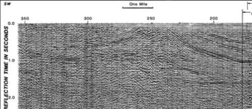
(After Applegate and Ross, in Gries and Dyer 1985. Published by permission of the Rocky Mountain Association of Geologists and the Denver Geophysical Society.)
Figure 10-50. Seismic section imaging a triangle zone to the right of sp 250, Raton Basin, Colorado.
Medwedeff (1988, 1989) extends the concept of interactive sole and roof thrusts to single structures, and he calls these interactive thrusts wedge structures. Figure 10-51a is an example of an incipient wedge structure that has two bends on its sole thrust and a single bend in its roof thrust. As the deformation progresses (Fig. 10-51b), motion along the sole thrust deforms the roof thrust. Back and frontal dip panels form over what is essentially a fault bend fold that also has an upper roof detachment. Notice, however, that the overlying beds in effect ride up the roof thrust, and they will also form fold panels above the upper detachment. This structurally higher fold is caused by the bends in the roof thrust, so its dip panels terminate at the upper detachment (Fig. 10-51b). The result is two folds for the price of one, which are slightly offset from each other. As the deformation progresses (Fig. 10-51c), the axial surfaces interfere and annihilate each other as they form branch points. This example illustrates that the deformation process can be very transient, and that the introduction of additional fault bends results in folds that have more rounded tops (Fig. 10-51c). Medwedeff (1988) uses wedge structures to model the complex stratigraphic relationships present at Wheeler Ridge, California. The restored structure and the present structure, with the corresponding positions of the wells (with their well logs), are shown in Figs. 10-52 and 10-53 respectively. These figures demonstrate how well logs can be used to define the complex relationships that exist within some structures. Precise correlations and balancing can be effectively integrated to locate prospects that may not be recognized by normal mapping techniques.

(Published by permission of Don Medwedeff 1988.)
Figure 10-51. Wedge structure showing progressive stages of development.

(Published by permission of Don Medwedeff 1988.)
Figure 10-52. Wedge structure in its initial, or restored, state as defined by well logs; Wheeler Ridge, California, USA.

(Published by permission of Don Medwedeff 1988.)
Figure 10-53. Wedge structure in its present state as defined by well logs, Wheeler Ridge, California, USA.
Would you believe that anticlines can form over synclines with no evidence of an intervening fault or evidence of more than one deformation? Nevertheless, clear evidence for this seemingly contradictory relationship can be seen on seismic sections and in outcrops. In the previous section on wedge structures, we saw that deformation on a lower level can modify the shape and the form of dip panels of structures located on a higher structural level. Where structural modification of this type results from a single deformation along one thrust surface, as illustrated in Fig. 10-54a, the resulting structures are called interference structures (Suppe 1988).

(Modified after Suppe 1988. Published by permission of John Suppe).
Figure 10-54. Interference structures (a) and (b) for clockwise deformation and increasing slip (c) for counterclockwise shear.
Interference structures are commonly present where the spacing between ramps is relatively narrow, causing the back dip panel of the leading structure to interfere with the frontal dip panel of the trailing structure (Fig. 10-54a and b). The interference tends to produce chevron folds and conjugate kink structures (Weiss 1972; Suppe 1988).
The resulting interference patterns that are created by the deformation are dependent on ramp spacing, initial cutoff angle, and the total amount of slip. Two model patterns are useful in mapping these types of structures, although this does not deny the usefulness of other types of patterns. In the first example, the leading fault bend fold has run up a ramp and the frontal dip panel of the trailing fold (a monocline) occupies a portion of the lower flat (Fig. 10-54a). The resulting deformation creates a structure in which a frontal fold lies beneath a structurally higher anticline formed by the trailing fold. Flat dips and a syncline exist just above the lower flat, directly in front of the trailing monocline.
As the deformation progresses, the frontal portions of the trailing monocline will start to run up the leading ramp (Fig. 10-54b). If both ramps have about the same cutoff angle, then as the trailing monocline runs up the second ramp, the beds in the frontal dip panel of the trailing monocline will flatten. One result of the deformation is to create a region of nearly flat dips and a narrow syncline over the leading ramp as the monocline unfolds. This example once again stresses the progressive nature of the deformation. Structures were not cast in their present-day positions; they move, and thus strata bend and rebend. Knowledge of which regions of a fold have been subject to refolding should aid in the prediction of fracture porosities and better well site locations, which can result in greater productivity. In our example, some of the strata in the back dip panel of the leading fault bend fold were first bent backward, and then forward, by the advancing monocline. As the active axial surfaces sweep through the structure, particular regions within these folds will be subject to repeated deformation and bending that enhances fracture porosity. One can study the refolding by applying the kink method and by modeling increasing amounts of slip into the structure to study how the deformation progresses.
We make two more points before leaving this subject. First, as the initial cutoff angle decreases, the structurally higher anticline will move vertically away from the structurally lower syncline, but at the same time shift to a position where it is located almost directly above the syncline. Second, the two examples presented here are for a clockwise shear within the interfering frontal and back dip panels. In other words, the beds within the interfering dip panels exhibit a “Z” vergence (Suppe 1988). An example of an “S” vergence (counterclockwise shear), in which the frontal dip panel of the trailing monocline passes through the upper anticline, is shown in Fig. 10-54c.