Context-Free Grammars

We can use grammars to specify different rules that allow us to build up parts-of-speech into phrases or chunks. A context-free grammar is a set of rules for combining syntactic components to form sensical strings. For instance, the noun phrase “the castle” has a determiner (denoted DT using the Penn Treebank tagset) and a noun (N). The prepositional phrase (PP) “in the castle” has a preposition (P) and a noun phrase (NP). The verb phrase (VP) “looks in the castle” has a verb (V) and a prepositional phrase (PP). The sentence (S) “Gwen looks in the castle” has a proper noun (NNP) and verb phrase (VP). Using these tags, we can define a context-free grammar:

GRAMMAR = """
    S -> NNP VP
    VP -> V PP
    PP -> P NP
    NP -> DT N
    NNP -> 'Gwen' | 'George'
    V -> 'looks' | 'burns'
    P -> 'in' | 'for'
    DT -> 'the'
    N -> 'castle' | 'ocean'
    """

In NLTK, nltk.grammar.CFG is an object that defines a context-free grammar, specifying how different syntactic components can be related. We can use CFG to parse our grammar as a string:

from nltk import CFG
cfg = nltk.CFG.fromstring(GRAMMAR)

print(cfg)
print(cfg.start())
print(cfg.productions())

Syntactic Parsers

Once we have defined a grammar, we need a mechanism to systematically search out the meaningful syntactic structures from our corpus; this is the role of the parser. If a grammar defines the search criterion for “meaningfulness” in the context of our language, the parser executes the search. A syntactic parser is a program that deconstructs sentences into a parse tree, which consists of hierarchical constituents, or syntactic categories.

When a parser encounters a sentence, it checks to see if the structure of that sentence conforms to a known grammar. If so, it parses the sentence according to the rules of that grammar, producing a parse tree. Parsers are often used to identify important structures, like the subject and object of verbs in a sentence, or to determine which sequences of words in a sentence should be grouped together within each syntactic category.

First, we define a GRAMMAR to identify sequences of text that match a part-of-speech pattern, and then instantiate an NLTK RegexpParser that uses our grammar to chunk the text into subsections:

from nltk.chunk.regexp import RegexpParser

GRAMMAR = r'KT: {(<JJ>* <NN.*>+ <IN>)? <JJ>* <NN.*>+}'
chunker = RegexpParser(GRAMMAR)

The GRAMMAR is a regular expression used by the NLTK RegexpParser to create trees with the label KT (key term). Our chunker will match phrases that start with an optional component composed of zero or more adjectives, followed by one or more of any type of noun and a preposition, and end with zero or more adjectives followed by one more of any type of noun. This grammar will chunk phrases like “red baseball bat” or “United States of America.”

Consider an example sentence from a news story about baseball: “Dusty Baker proposed a simple solution to the Washington National’s early-season bullpen troubles Monday afternoon and it had nothing to do with his maligned group of relievers.”

(S
  (KT Dusty/NNP Baker/NNP)
  proposed/VBD
  a/DT
  (KT simple/JJ solution/NN)
  to/TO
  the/DT
  (KT Washington/NNP Nationals/NNP)
  (KT
    early-season/JJ
    bullpen/NN
    troubles/NNS
    Monday/NNP
    afternoon/NN)
  and/CC
  it/PRP
  had/VBD
  (KT nothing/NN)
  to/TO
  do/VB
  with/IN
  his/PRP$
  maligned/VBN
  (KT group/NN of/IN relievers/NNS)
  ./.)

This sentence is parsed into keyphrase chunks with six key phrases, including “Dusty Baker,” “early-season bullpen troubles Monday afternoon,” and “group of relievers.”

Extracting Keyphrases

Figure 4-8 depicted a pipeline that included a feature union with a KeyphraseExtractor and an EntityExtractor. In this section, we’ll implement the KeyphraseExtractor class that will transform documents into a bag-of-keyphrase representation.

The key terms and keyphrases contained within our corpora often provide insight into the topics or entities contained in the documents being analyzed. Keyphrase extraction consists of identifying and isolating phrases of a dynamic size to capture as many nuances in the topics of documents as possible.

The first step in keyphrase extraction is to identify candidates for phrases (e.g., which words or phrases could best convey the topic or relationships of documents). We’ll define our KeyphraseExtractor with a grammar and chunker to identify just the noun phrases using part-of-speech tagged text.

GRAMMAR = r'KT: {(<JJ>* <NN.*>+ <IN>)? <JJ>* <NN.*>+}'
GOODTAGS = frozenset(['JJ','JJR','JJS','NN','NNP','NNS','NNPS'])

class KeyphraseExtractor(BaseEstimator, TransformerMixin):
    """
    Wraps a PickledCorpusReader consisting of pos-tagged documents.
    """
    def __init__(self, grammar=GRAMMAR):
        self.grammar = GRAMMAR
        self.chunker = RegexpParser(self.grammar)

Since we imagine that this KeyphraseExtractor will be the first step in a pipeline after tokenization, we’ll add a normalize() method that performs some lightweight text normalization, removing any punctuation and ensuring that all words are lowercase:

from unicodedata import category as unicat

    def normalize(self, sent):
        """
        Removes punctuation from a tokenized/tagged sentence and
        lowercases words.
        """
        is_punct = lambda word: all(unicat(c).startswith('P') for c in word)
        sent = filter(lambda t: not is_punct(t[0]), sent)
        sent = map(lambda t: (t[0].lower(), t[1]), sent)
        return list(sent)

Now we will write an extract_keyphrases() method. Given a document, this method will first normalize the text and then use our chunker to parse it. The output of a parser is a tree with only some branches of interest (the keyphrases!). To get the phrases of interest, we use the tree2conlltags function to convert the tree into the CoNLL IOB tag format, a list containing (word, tag, IOB-tag) tuples.

An IOB tag tells you how a term is functioning in the context of the phrase; the term will either begin a keyphrase (B-KT), be inside a keyphrase (I-KT), or be outside a keyphrase (O). Since we’re only interested in the terms that are part of a keyphrase, we’ll use the groupby() function from the itertools package in the standard library to write a lambda function that continues to group terms so long as they are not O:

from itertools import groupby
from nltk.chunk import tree2conlltags

    def extract_keyphrases(self, document):
        """
        For a document, parse sentences using our chunker created by
        our grammar, converting the parse tree into a tagged sequence.
        Yields extracted phrases.
        """
        for sents in document:
            for sent in sents:
                sent = self.normalize(sent)
                if not sent: continue
                chunks = tree2conlltags(self.chunker.parse(sent))
                phrases = [
                    " ".join(word for word, pos, chunk in group).lower()
                    for key, group in groupby(
                        chunks, lambda term: term[-1] != 'O'
                    ) if key
                ]
                for phrase in phrases:
                    yield phrase

Since our class is a transformer, we finish by adding a no-op fit method and a transform method that calls extract_keyphrases() on each document in the corpus:

    def fit(self, documents, y=None):
        return self

    def transform(self, documents):
        for document in documents:
            yield self.extract_keyphrases(document)

Here’s a sample result for one of our transformed documents:

['lonely city', 'heart piercing wisdom', 'loneliness', 'laing',
'everyone', 'feast later', 'point', 'own hermetic existence in new york',
'danger', 'thankfully', 'lonely city', 'cry for connection',
'overcrowded overstimulated world', 'blueprint of urban loneliness',
'emotion', 'calls', 'city', 'npr jason heller', 'olivia laing',
'lonely city', 'exploration of loneliness',
'others experiences in new york city', 'rumpus', 'review', 'lonely city',
'related posts']

In Chapter 12, we’ll revisit this class with a different GRAMMAR to build a custom bag-of-keyphrase transformer for a neural network-based sentiment classifier.

Extracting Entities

Similarly to our KeyphraseExtractor, we can create a custom feature extractor to transform documents into bags-of-entities. To do this we will make use of NLTK’s named entity recognition utility, ne_chunk, which produces a nested parse tree structure containing the syntactic categories as well as the part-of-speech tags contained in each sentence.

We begin by creating an EntityExtractor class that is initialized with a set of entity labels. We then add a get_entities method that uses ne_chunk to get a syntactic parse tree for a given document. The method then navigates through the subtrees in the parse tree, extracting entities whose labels match our set (consisting of people’s names, organizations, facilities, geopolitical entities, and geosocial political entities). We append these to list of entities, which we yield after the method has finished traversing all the trees of the document:

from nltk import ne_chunk

GOODLABELS = frozenset(['PERSON', 'ORGANIZATION', 'FACILITY', 'GPE', 'GSP'])

class EntityExtractor(BaseEstimator, TransformerMixin):
    def __init__(self, labels=GOODLABELS, **kwargs):
        self.labels = labels

    def get_entities(self, document):
        entities = []
        for paragraph in document:
            for sentence in paragraph:
                trees = ne_chunk(sentence)
                for tree in trees:
                    if hasattr(tree, 'label'):
                        if tree.label() in self.labels:
                            entities.append(
                                ' '.join([child[0].lower() for child in tree])
                                )
        return entities

    def fit(self, documents, labels=None):
        return self

    def transform(self, documents):
        for document in documents:
            yield self.get_entities(document)

A sample document from our transformed corpus looks like:

['lonely city', 'loneliness', 'laing', 'new york', 'lonely city',
'npr', 'jason heller', 'olivia laing', 'lonely city', 'new york city',
'rumpus', 'lonely city', 'related']

We will revisit grammar-based feature extraction in Chapter 9, where we’ll make use of our EntityExtractor for use with graph metrics to model the relative importances of different entities in documents.

An n-Gram-Aware CorpusReader

n-gram extraction is part of text preprocessing that occurs prior to modeling. As such, it would be convenient to include an ngrams() method as part of our custom CorpusReader and PickledCorpusReader classes. This will ensure it is easy to process our entire corpus for n-grams and retrieve them later. For example:

class HTMLCorpusReader(CategorizedCorpusReader, CorpusReader):

    ...

    def ngrams(self, n=2, fileids=None, categories=None):
        for sent in self.sents(fileids=fileids, categories=categories):
            for ngram in nltk.ngrams(sent, n):
                yield ngram

    ...

Because we are primarily considering context and because sentences represent discrete and independent thoughts, it makes sense to consider n-grams that do not cross over sentence boundaries.

The easiest way to handle more complex n-gram manipulation is to use the ngrams() method from NLTK, which can be used alongside NLTK segmentation and tokenization methods. This method will enable us to add padding before and after sentences such that n-grams generated also include sentence boundaries. This will allow us to identify which n-grams start sentences and which conclude them.

We’ll begin with constants to define the start and end of the sentence as <s> and </s> (because English reads left to right, the left_pad_symbol and right_pad_symbol, respectively). In languages that read right to left, these could be reversed.

The second part of the code creates a function nltk_ngrams that uses the partial function to wrap the nltk.ngrams function with our code-specific keyword arguments. This ensures that every time we call nltk_ngrams, we get our expected behavior, without managing the call signature everywhere in our code that we use it. Finally our newly redefined ngrams function takes as arguments a string containing our text and n-gram size. It then applies the sent_tokenize and word_tokenize functions to the text before passing them into nltk_ngrams to get our padded n-grams:

import nltk
from functools import partial

LPAD_SYMBOL = "<s>"
RPAD_SYMBOL = "</s>"

nltk_ngrams = partial(
    nltk.ngrams,
    pad_right=True, right_pad_symbol=RPAD_SYMBOL,
    left_pad=True, left_pad_symbol=LPAD_SYMBOL
)

    def ngrams(self, n=2, fileids=None, categories=None):
        for sent in self.sents(fileids=fileids, categories=categories):
            for ngram in nltk.ngrams(sent, n):
                yield ngram

For instance, given a size of n=4 and the sample text, “After, there were several follow-up questions. The New York Times asked when the bill would be signed,” the resulting four-grams would be:

('<s>', '<s>', '<s>', 'After')
('<s>', '<s>', 'After', ',')
('<s>', 'After', ',', 'there')
('After', ',', 'there', 'were')
(',', 'there', 'were', 'several')
('there', 'were', 'several', 'follow')
('were', 'several', 'follow', 'up')
('several', 'follow', 'up', 'questions')
('follow', 'up', 'questions', '.')
('up', 'questions', '.', '</s>')
('questions', '.', '</s>', '</s>')
('.', '</s>', '</s>', '</s>')
('<s>', '<s>', '<s>', 'The')
('<s>', '<s>', 'The', 'New')
('<s>', 'The', 'New', 'York')
('The', 'New', 'York', 'Times')
('New', 'York', 'Times', 'asked')
('York', 'Times', 'asked', 'when')
('Times', 'asked', 'when', '</s>')
('asked', 'when', '</s>', '</s>')
('when', '</s>', '</s>', '</s>')

Note that the padding function adds padding to all possible sequences of n-grams. While this will be useful later in our discussion of backoff, if your application only requires identification of the start and end of the sentence, you can simply filter n-grams that contain more than one padding symbol.

Choosing the Right n-Gram Window

So how do we decide which n to choose? Consider an application where we are using n-grams to identify candidates for named entity recognition. If we consider a chunk size of n=2, our results include “The reporters,” “the President,” “the United,” and “the room.” While not perfect, this model successfully identifies three of the relevant entities as candidates in a lightweight fashion.

On the other hand, a model based on the small n-gram window of 2 would fail to capture some of the nuance of the original text. For instance, if our sentence is from a text that references multiple heads of state, “the President” could be somewhat ambiguous. In order to capture the entirety of the phrase “the President of the United States,” we would have to set n=6:

('The', 'reporters', 'listened', 'closely', 'as', 'the'),
('reporters', 'listened', 'closely', 'as', 'the', 'President'),
('listened', 'closely', 'as', 'the', 'President', 'of'),
('closely', 'as', 'the', 'President', 'of', 'the'),
('as', 'the', 'President', 'of', 'the', 'United'),
('the', 'President', 'of', 'the', 'United', 'States'),
('President', 'of', 'the', 'United', 'States', 'addressed'),
('of', 'the', 'United', 'States', 'addressed', 'the'),
('the', 'United', 'States', 'addressed', 'the', 'room'),
('United', 'States', 'addressed', 'the', 'room', '.')

Unfortunately, as we can see in the results above, if we build a model based on an n-gram order that is too high, it will be very unlikely that we’ll see any repeated entities. This will make it very difficult to assign likelihoods that capture the target of our analysis. Moreover, as n increases, the number of possible correct n-grams increases, thereby reducing the likelihood that we will observe all correct n-grams in our corpus. Too large of an n may add too much noise by overlapping independent contexts. If the window is larger than the sentence, it might not even produce any n-grams at all.

Choosing n can also be considered as balancing the trade-off between bias and variance. A small n leads to a simpler (weaker) model, therefore causing more error due to bias. A larger n leads to a more complex model (a higher-order model), thus causing more error due to variance. Just as with all supervised machine learning problems, we have to strike the right balance between the sensitivity and the specificity of our model. The more dependent words are on more distant precursors, the greater the complexity needed for an n-gram model to be predictive.

Significant Collocations

Now that our corpus reader is aware of n-grams, we can incorporate these features into our downstream models by vectorizing our text using n-grams as vector elements instead of simply vocabulary. However, using raw n-grams will produce many, many candidates, most of which will not be relevant. For example, the sentence “I got lost in the corn maze during the fall picnic” contains the trigram ('in', 'the', 'corn'), which is not a typical prepositional target, whereas the trigram ('I', 'got', 'lost') seems to make sense on its own.

In practice, this is too high a computational cost to be useful in most applications. The solution is to compute conditional probability. For example, what is the likelihood that the tokens ('the', 'fall') appear in the text given the token 'during'? We can compute empirical likelihoods by calculating the frequency of the (n-1)-gram conditioned by the first token of the n-gram. Using this technique we can value n-grams that are more often used together such as ('corn', 'maze') over rarer compositions that are less meaningful.

The idea of some n-grams having more value than others leads to another tool in the text analysis toolkit: significant collocations. Collocation is an abstract synonym for n-gram (without the specificity of the window size) and simply means a sequence of tokens whose likelihood of co-occurrence is caused by something other than random chance. Using conditional probability, we can test the hypothesis that a specified collocation is meaningful.

NLTK contains two tools to discover significant collocations: the CollocationFinder, which finds and ranks n-gram collocations, and NgramAssocMeasures, which contains a collection of metrics to score the significance of a collocation. Both utilities are dependent on the size of n and the module contains bigram, trigram, and quadgram ranking utilities. Unfortunately, 5-gram associations and above must be manually implemented by subclassing the correct base class and using one of the collocation tools as a template.

For now, let’s explore the discovery of significant quadgrams. Because finding and ranking n-grams for a large corpus can take a lot of time, it is a good practice to write the results to a file on disk. We’ll create a rank_quadgrams function that takes as input a corpus to read words from, as well as a metric from the QuadgramAssocMeasures, finds and ranks quadgrams, then writes the results as a tab-delimited file to disk:

from nltk.collocations import QuadgramCollocationFinder
from nltk.metrics.association import QuadgramAssocMeasures


def rank_quadgrams(corpus, metric, path=None):
    """
    Find and rank quadgrams from the supplied corpus using the given
    association metric. Write the quadgrams out to the given path if
    supplied otherwise return the list in memory.
    """
    # Create a collocation ranking utility from corpus words.
    ngrams = QuadgramCollocationFinder.from_words(corpus.words())

    # Rank collocations by an association metric
    scored = ngrams.score_ngrams(metric)

    if path:
        # Write to disk as tab-delimited file
        with open(path, 'w') as f:
            f.write("Collocation	Score ({})".format(metric.__name__))
            for ngram, score in scored:
                f.write("{}	{}
".format(repr(ngram), score))
    else:
        return scored

For example, we could use the likelihood ratios metric as follows:

rank_quadgrams(
    corpus, QuadgramAssocMeasures.likelihood_ratio, 'quadgrams.txt'
)

This produces quadgrams with likelihood scores from our sample corpus, a few samples of which follow:

Collocation Score (likelihood_ratio)
('New', 'York', "'", 's') 156602.26742890902
('pictures', 'of', 'the', 'Earth')      28262.697780596758
('the', 'majority', 'of', 'users')      28262.36608379526
('numbed', 'by', 'the', 'mindlessness') 3091.139615301832
('There', 'was', 'a', 'time')   3090.2332736791095

The QuadgramAssocMeasures class gives several methods with which to rank significance via hypothesis testing. These methods assume that there is no association between the words (e.g., the null hypothesis), then compute the probability of the association occurring if the null hypothesis was true. If we can reject the null hypothesis because its significance level is too low we can accept the alternative hypothesis.

Now we can conceive of a SignificantCollocations feature extraction transformer for use in a pipeline such as the one shown in Figure 7-2.

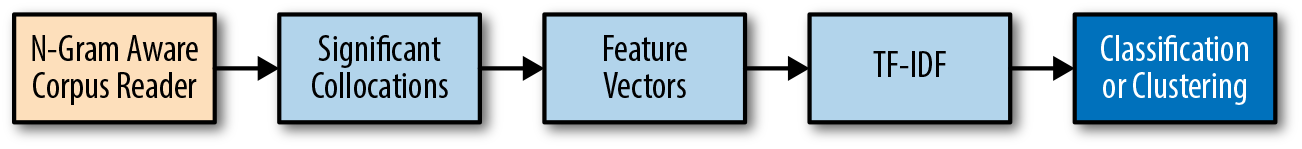
Figure 7-2. An n-gram feature extraction pipeline

On fit(), it would find and rank significant collocations, and then on transform() produce a vector that encoded the score for any significant collocation found in the document. These features could then be joined to your other vectors using the FeatureUnion.

from sklearn.base import BaseEstimator, TransformerMixin


class SignificantCollocations(BaseEstimator, TransformerMixin):

    def __init__(self,
                 ngram_class=QuadgramCollocationFinder,
                 metric=QuadgramAssocMeasures.pmi):
        self.ngram_class = ngram_class
        self.metric = metric

    def fit(self, docs, target):
        ngrams = self.ngram_class.from_documents(docs)
        self.scored_ = dict(ngrams.score_ngrams(self.metric))

    def transform(self, docs):
        for doc in docs:
            ngrams = self.ngram_class.from_words(docs)
            yield {
                ngram: self.scored_.get(ngram, 0.0)
                for ngram in ngrams.nbest(QuadgramAssocMeasures.raw_freq, 50)
            }

The model could then be composed as follows:

from sklearn.linear_model import SGDClassifier
from sklearn.pipeline import Pipeline, FeatureUnion
from sklearn.feature_extraction import DictVectorizer
from sklearn.feature_extraction.text import TfidfVectorizer


model = Pipeline([
    ('union', FeatureUnion(
        transformer_list=[
            ('ngrams', Pipeline([
                ('sigcol', SignificantCollocations()),
                ('dsigcol', DictVectorizer()),
            ])),

            ('tfidf', TfidfVectorizer()),
        ]
    ))

    ('clf', SGDClassifier()),
])

Note that this is stub code only, but hopefully serves as a template so that context can be easily injected into a standard bag of words model.

Frequency and Conditional Frequency

We first explored the concept of token frequency in Figure 4-2, where we used frequency representations with our bag-of-words model with the assumption that word count could sufficiently approximate a document’s contents to differentiate it from others. Frequency is also a useful feature with n-gram modeling, where the frequency with which an n-gram occurs in the training corpus might reasonably lead us to expect to see that n-gram in new documents.

Imagine we are reading a book one word at a time and we want to compute the probability of the next word we’ll see. A naive choice would be to assign the highest probability to the words that appear most frequently in the text, which we can visualize in Figure 7-3.

Figure 7-3. Frequency distribution plot of a text corpus

However, we know that this basic use of frequency is not enough; if we’re starting a sentence some words have higher probability than other words and some words are much more likely given preceding words. For example, asking the question what is the probability of the word “chair” following “lawn” is very different than the probability of the word “chair” following “lava” (or “lamp”). These likelihoods are informed by conditional probabilities and are formulated as P(chair|lawn) (read as “the probability of chair given lawn”). To model these probabilities, we need to be able to compute the conditional frequencies of each of the possible n-gram windows.

We begin by defining an NgramCounter class that can keep track of conditional frequencies of all subgrams from unigrams up to n-grams using FreqDist and ConditionalFreqDist. Our class also implements the sentence padding we explored earlier in the chapter, and detects words that are not in the vocabulary of the original corpus.

from nltk.util import ngrams
from nltk.probability import FreqDist, ConditionalFreqDist

from collections import defaultdict

# Padding Symbols
UNKNOWN = "<UNK>"
LPAD = "<s>"
RPAD = "</s>"


class NgramCounter(object):
    """
    The NgramCounter class counts ngrams given a vocabulary and ngram size.
    """

    def __init__(self, n, vocabulary, unknown=UNKNOWN):
        """
        n is the size of the ngram
        """
        if n < 1:
            raise ValueError("ngram size must be greater than or equal to 1")

        self.n = n
        self.unknown = unknown
        self.padding = {
            "pad_left": True,
            "pad_right": True,
            "left_pad_symbol": LPAD,
            "right_pad_symbol": RPAD,
        }

        self.vocabulary = vocabulary
        self.allgrams = defaultdict(ConditionalFreqDist)
        self.ngrams = FreqDist()
        self.unigrams = FreqDist()

Next, we will create a method for the NgramCounter class that enables us to systematically compute the frequency distribution and conditional frequency distribution for the requested n-gram window.

    def train_counts(self, training_text):
        for sent in training_text:
            checked_sent = (self.check_against_vocab(word) for word in sent)
            sent_start = True
            for ngram in self.to_ngrams(checked_sent):
                self.ngrams[ngram] += 1
                context, word = tuple(ngram[:-1]), ngram[-1]
                if sent_start:
                    for context_word in context:
                        self.unigrams[context_word] += 1
                    sent_start = False

                for window, ngram_order in enumerate(range(self.n, 1, -1)):
                    context = context[window:]
                    self.allgrams[ngram_order][context][word] += 1
                self.unigrams[word] += 1

    def check_against_vocab(self, word):
        if word in self.vocabulary:
            return word
        return self.unknown

    def to_ngrams(self, sequence):
        """
        Wrapper for NLTK ngrams method
        """
        return ngrams(sequence, self.n, **self.padding)

Now we can define a quick method (outside of our NgramCounter class definition) that instantiates the counter and computes the relevant frequencies. Our count_ngrams function takes as parameters the desired n-gram size, the vocabulary, and a list of sentences represented as comma-separated strings.

def count_ngrams(n, vocabulary, texts):
    counter = NgramCounter(n, vocabulary)
    counter.train_counts(texts)
    return counter

if __name__ == '__main__':
    corpus = PickledCorpusReader('../corpus')
    tokens = [''.join(word[0]) for word in corpus.words()]
    vocab = Counter(tokens)
    sents = list([word[0] for word in sent] for sent in corpus.sents())
    trigram_counts = count_ngrams(3, vocab, sents)

For unigrams, we can get the frequency distribution using the unigrams attribute.

print(trigram_counts.unigrams)

For n-grams of higher order, we can retrieve a conditional frequency distribution from the ngrams attribute.

print(trigram_counts.ngrams[3])

The keys of the conditional frequency distribution show the possible contexts that might precede each word.

print(sorted(trigram_counts.ngrams[3].conditions()))

We can also use our model to get the list of possible next words:

print(list(trigram_counts.ngrams[3][('the', 'President')]))

Estimating Maximum Likelihood

Our NgramCounter class gives us the ability to transform a corpus into a conditional frequency distribution of n-grams. In the context of our hypothetical next word prediction application, we need a mechanism for scoring the possible candidates for next words after an n-gram so we can provide the most likely. In other words, we need a model that computes the probability of a token, t, given a preceding sequence, s.

One straightforward way to estimate the probability of the n-gram (s,t) is by computing its relative frequency. This is the number of times we see t appear as the next word after s in the corpus, divided by the total number of times we observe s in the corpus. The resulting ratio gives us a maximum likelihood estimate for the n-gram (s,t).

We will start by creating a class, BaseNgramModel, that will take as input an NgramCounter object and produce a language model. We will initialize the BaseNgramModel model with attributes to keep track of the highest order n-grams from the trained NgramCounter, as well as the conditional frequency distributions of the n-grams, the n-grams themselves, and the vocabulary.

class BaseNgramModel(object):
    """
    The BaseNgramModel creates an n-gram language model.
    """

    def __init__(self, ngram_counter):
        """
        BaseNgramModel is initialized with an NgramCounter.
        """
        self.n = ngram_counter.n
        self.ngram_counter = ngram_counter
        self.ngrams = ngram_counter.ngrams[ngram_counter.n]
        self._check_against_vocab = self.ngram_counter.check_against_vocab

Next, inside our BaseNgramModel class, we create a score method to compute the relative frequency for the word given the context, checking first to make sure that the context is always shorter than the highest order n-grams from the trained NgramCounter. Since the ngrams attribute of the BaseNgramModel is an NLTK ConditionalFreqDist, we can retrieve the FreqDist for any given context, and get its relative frequency with freq:

    def score(self, word, context):
        """
        For a given string representation of a word, and a string word context,
        returns the maximum likelihood score that the word will follow the
        context.

        fdist[context].freq(word) == fdist[(context, word)] / fdist[context]
        """
        context = self.check_context(context)

        return self.ngrams[context].freq(word)

    def check_context(self, context):
        """
        Ensures that the context is not longer than or equal to the model's
        highest n-gram order.

        Returns the context as a tuple.
        """
        if len(context) >= self.n:
            raise ValueError("Context too long for this n-gram")

        return tuple(context)

In practice, n-gram probabilities tend to be pretty small, so they are often represented as log probabilities instead. For this reason, we’ll create a logscore method that transforms the result of our score method into log format, unless the score is less than or equal to zero, in which case we’ll return negative infinity:

    def logscore(self, word, context):
        """
        For a given string representation of a word, and a word context,
        computes the log probability of the word in the context.
        """
        score = self.score(word, context)
        if score <= 0.0:
            return float("-inf")

        return log(score, 2)

Now that we have methods for scoring instances of particular n-grams, we want a method to score the language model as a whole, which we will do with entropy. We can create an entropy method for our BaseNgramModel by taking the average log probability of every n-gram from our NgramCounter.

    def entropy(self, text):
        """
        Calculate the approximate cross-entropy of the n-gram model for a
        given text represented as a list of comma-separated strings.
        This is the average log probability of each word in the text.
        """
        normed_text = (self._check_against_vocab(word) for word in text)
        entropy = 0.0
        processed_ngrams = 0
        for ngram in self.ngram_counter.to_ngrams(normed_text):
            context, word = tuple(ngram[:-1]), ngram[-1]
            entropy += self.logscore(word, context)
            processed_ngrams += 1
        return - (entropy / processed_ngrams)

In Chapter 1 we encountered the concept of perplexity, and considered that within a given utterance, the previous few words might be enough to predict the next few subsequent words. The primary assumption is that meaning is very local, which is a variation of the Markov assumption. In the case of an n-gram model, we want to minimize perplexity by selecting the most likely (n+1)-gram, given an input n-gram. For that reason, it is common to evaluate the predictive power of a model by measuring its perplexity, which we can compute in terms of entropy, as 2 to the power entropy:

    def perplexity(self, text):
        """
        Given list of comma-separated strings, calculates the perplexity
        of the text.
        """
        return pow(2.0, self.entropy(text))

Perplexity is a normalized way of computing probability; the higher the conditional probability of a sequence of tokens, the lower its perplexity will be. We should expect to see our higher-order models demonstrate less perplexity than our weaker models:

trigram_model = BaseNgramModel(count_ngrams(3, vocab, sents))
fivegram_model = BaseNgramModel(count_ngrams(5, vocab, sents))

print(trigram_model.perplexity(sents[0]))
print(fivegram_model.perplexity(sents[0]))

Unknown Words: Back-off and Smoothing

Because natural language is so flexible, it would be naive to expect even a very large corpus to contain all possible n-grams. Therefore our models must also be sufficiently flexible to deal with n-grams it has never seen before (e.g., “the President of California,” “the United States of Canada”). Symbolic models deal with this problem of coverage through backoff—if the probability for an n-gram does not exist, the model looks for the probability of the (n-1)-gram (“the President of,” “the United States of”), and so forth, until it gets to single tokens, or unigrams. As a rule of thumb, we should recursively back off to smaller n-grams until we have enough data to get a probability estimate.

Since our BaseNgramModel uses maximum likelihood estimation, some (perhaps many) n-grams will have a zero probability of occurring, resulting in a score() of zero and a perplexity score of + or - infinity. The means of addressing these zero-probability n-grams is to implement smoothing. Smoothing consists of donating some of the probability mass of frequent n-grams to unseen n-grams. The simplest type of smoothing is “add-one,” or Laplace, smoothing, where the new term is assigned a frequency of 1 and the probabilities are recomputed, but there are many other types, such as “add-k,” which is a generalization of Laplace smoothing.

We can easily implement both by creating an AddKNgramModel that inherits from our BaseNgramModel and overrides the score method by adding the smoothing value k to the n-gram count and dividing by the (n-1)-gram count, normalized by the unigram count multiplied by k:

class AddKNgramModel(BaseNgramModel):
    """
    Provides add-k smoothed scores.
    """
    def __init__(self, k, *args):
        """
        Expects an input value, k, a number by which
        to increment word counts during scoring.
        """
        super(AddKNgramModel, self).__init__(*args)

        self.k = k
        self.k_norm = len(self.ngram_counter.vocabulary) * k

    def score(self, word, context):
        """
        With Add-k-smoothing, the score is normalized with
        a k value.
        """
        context = self.check_context(context)
        context_freqdist = self.ngrams[context]
        word_count = context_freqdist[word]
        context_count = context_freqdist.N()
        return (word_count + self.k) / 
               (context_count + self.k_norm)

Then we can create a LaplaceNgramModel class by passing in a value of k=1 to our AddKNgramModel:

class LaplaceNgramModel(AddKNgramModel):
    """
    Implements Laplace (add one) smoothing.
    Laplace smoothing is the base case of add-k smoothing,
    with k set to 1.
    """
    def __init__(self, *args):
        super(LaplaceNgramModel, self).__init__(1, *args)

NLTK’s probability module exposes a number of ways of calculating probability, including some variations on maximum likelihood and add-k smoothing, as well as:

• UniformProbDist, which assigns equal probability to every sample in a given set, and a zero probability to all other samples.

• LidstoneProbDist, which smooths sample probabilities using a real number gamma between 0 and 1.

• KneserNeyProbDist, which implements a version of back-off that counts how likely an n-gram is provided the (n-1)-gram has been seen in training.

Kneser–Ney smoothing considers the frequency of a unigram not by itself but in relation to the n-grams it completes. While some words appear in many different contexts, others appear frequently, but only in certain contexts; we want to treat these differently.

We can create a wrapper for NLTK’s convenient implementation of Kneser–Ney smoothing by creating a class KneserNeyModel that inherits from BaseNgramModel and overrides the score method to use nltk.KneserNeyProbDist. Note that NLTK’s implementation, nltk.KneserNeyProbDist, requires trigrams:

class KneserNeyModel(BaseNgramModel):
    """
    Implements Kneser-Ney smoothing
    """
    def __init__(self, *args):
        super(KneserNeyModel, self).__init__(*args)
        self.model = nltk.KneserNeyProbDist(self.ngrams)

    def score(self, word, context):
        """
        Use KneserNeyProbDist from NLTK to get score
        """
        trigram = tuple((context[0], context[1], word))
        return self.model.prob(trigram)

Language Generation

Once we can assign probabilities to n-grams, we have a mechanism for preliminary language generation. In order to apply our KneserNeyModel to build a next word generator, we will create two additional methods, samples and prob, so that we can access the list of all trigrams with nonzero probabilities and the probability of each sample.

    def samples(self):
        return self.model.samples()

    def prob(self, sample):
        return self.model.prob(sample)

Now, we can create a simple function that takes input text, retrieves the probability of each possible trigram continuation of the last two words, and appends the most likely next word. If fewer than two words are provided, we ask for more input. If our KneserNeyModel assigns zero probability, we try to change the subject:

corpus = PickledCorpusReader('../corpus')
tokens = [''.join(word) for word in corpus.words()]
vocab = Counter(tokens)
sents = list([word[0] for word in sent] for sent in corpus.sents())

counter = count_ngrams(3, vocab, sents)
knm = KneserNeyModel(counter)

def complete(input_text):
    tokenized = nltk.word_tokenize(input_text)
    if len(tokenized) < 2:
        response = "Say more."
    else:
        completions = {}
        for sample in knm.samples():
            if (sample[0], sample[1]) == (tokenized[-2], tokenized[-1]):
                completions[sample[2]] = knm.prob(sample)
        if len(completions) == 0:
            response = "Can we talk about something else?"
        else:
            best = max(
                completions.keys(), key=(lambda key: completions[key])
            )
            tokenized += [best]
            response = " ".join(tokenized)

    return response

print(complete("The President of the United"))
print(complete("This election year will"))

The President of the United States
This election year will suddenly

While it’s fairly easy to construct an application that does simple probabilistic language generation tasks, we can see that to build anything much more complex (e.g., something that generates full sentences), it will be necessary to encode more about language. This can be achieved with higher-order n-gram models and larger, domain-specific corpora.

So how do we decide if our model is good enough? We can evaluate n-gram models in two ways. The first is by using a probability measure like perplexity or entropy to evaluate the performance of the model on held-out or test data. In this case, whichever model maximizes entropy or minimizes perplexity for the test set is the better performing model. It is customary to describe the performance of symbolic models by their maximal context in terms of the size of n-grams and their smoothing mechanism. At the time of this writing, the best performing symbolic models are variations of the Kneser–Ney smoothed 5-gram model.²

On the other hand, it is sometimes more effective to evaluate an n-model by integrating it into the application and having users give feedback!