
8
Deep Feature Selection for Wind Forecasting-II
S. Oswalt Manoj1*, J.P. Ananth2, Balan Dhanka3 and Maharaja Kamatchi4
1Department of Computer Science and Business System, Sri Krishna College of Engineering and Technology, Coimbatore, India
2Department of Computer Science and Engineering, Sri Krishna College of Engineering and Technology, Coimbatore, India
3University of Rajasthan, Rajasthan, India
4Engineering Department, University of Technology and Applied Sciences, Al Mussanah, Oman
Abstract
In recent years, large production of energy from renewable sources is significantly getting boosted in every part of the world. Due to the expeditious development of the penetration of the power related to wind into the present day power grid, the forecasting of wind speed turns into an expanding noteworthy assignment in power generation process. Accordingly, the scope of the chapter is to determine the forecasting of the wind speed in short term by incorporating the adaptive ensembles of Deep Neural Network, and the work is compared with the machine learning algorithms like Gated Recurrent Unit (GRU), Long Short-Term Memory Neural Network (LSTM), and Bidirectional Long Short-Term Memory Neural Network (Bi-LSTM). Various existing approaches for the forecasting of wind speed like physical and statistical models, along with artificial intelligence models is used by numerous researchers. The dataset has been received from various authenticated sources like Windmills in Jaipur, globalwindatlas.info and data.gov. in. It comprises of the parameters like time, dew point, wind speed, humidity, temperature (air), pressure, and month. This data can be used to determine the wind speed and the air density. Parameters like wind speed, blade swept area, and air density will be used to decide on the output power. The swept area is relied upon the design and the speed of the wind and air density has been predicted from the input data provided. Various parameters like the mean absolute error (MAE) and the root mean square error (RMSE) have been computed. Also, the mean square error (MSE) has been computed for the given algorithms, and the performance of the Bi-LSTM is comparatively good considering MSE, RMSE, and MAE.
Keywords: Deep learning, forecasting, wind speed, LSTM, deep neural network
8.1 Introduction
Energy crisis has hit the world and wind energy which is considered to be the renewable source is predictable as one of the feasible answer in order to see the energy crisis and it has attracted worldwide attention. The power from wind is produced throughout by the wind turbines by means of the flow of air. This is a noteworthy feature of the resources related to renewable energy because of the accessibility of wind turbines which is having even megawatt size, available facilities for management along with the subsidies by government, and low cost of maintenance. One of the most gifted renewable energy technologies has been normally considered. Wind speed is one among the major factors in the production of wind power. The operating cost can be increased based on the repeated and the variant characteristics of the wind speed, and also, the power system’s reliability could be challenged. The wind farms are to be protected and the scheduling of the power system also has to be improved. This can happen only by the accurate wind speed forecasting. The speed of wind is considered to be one of the difficult meteorological parameters to be predicted. The speed of wind is stochastic in nature and many complex factors can be may affect the same. Similarly, forecasting the speed of wind accurately is also a serious concern. During the recent years, abundant models related to wind speed have been established, and it can also be sorted into many varied categories conferring to varied principles.
The models that have been used for the prediction of wind speed are often categorized into three groups based on the time horizon prediction. These are as follows: the long-term future prediction models, the short-term future prediction models, and the medium-term prediction models. The future prediction models for the long-term prediction are utilized in the approximation capacity, and possibly, in selecting the location for the wind farm, the prediction models related to medium term are utilized specifically for the maintenance and operation of the wind farm and therefore the the future prediction models related to the short term are utilized in the optimal control of wind turbine, load decision, operational security, and also in the real-time operation of grid. It is also used to optimally control the wind turbine. On comparing all the three prediction models, the short term-wind speed prediction model requires less computation as compared with the medium- and long-term wind speed prediction models. So, most of the focus is on the short-term wind speed forecasting models. However, the standard uniqueness related to the models toward prediction of the wind speed play a vital role here. The prediction models related to wind speed are often branded into five categories of models, namely physical, conventional statistical, artificial intelligence (AI)–based, spatial correlation, and hybrid models along with the event of forecasting the wind speed. The models which are considered as hybrid has the ability to provide improved accuracy in prediction. The single models give least performance when it is compared with the hybrid models.
The precise and consistent methodology for forecasting wind generation supports the grid dispatching process, and it enhances the standard of the energy based on electricity. Current wind generation prediction methods are often categorized as physical, statistical, and combined physical statistical. A physical prediction model for wind generation considers the phenomena related to weather or the weather processes. The modeling can be done with the suitable laws related to physics which includes the momentum conservation and therefore the conservation of energy. The prediction of wind generation round the wind farm also requests the control of successive momentum of the positive state and it is attained by inspecting the atmospheric state which incorporates the neighboring air pressure, roughness, and temperature along with the obstacles. Based on the changes in the atmosphere, the numerical prediction of weather is done. Real-time environmental data is required because the physical prediction model is used for forecasting the wind generation. The data transmission network and the knowledge acquisition is in high demand always.
There is a complexity in the physical wind generation building process. The model is extremely subtle as far as the instruction is presented, and it is based on the standards. These standards of the physical data can be acquired as an alternate to the physical models. An equivalent weather might not induce an equivalent weather change. The weather changes can be treated as a random process at most of the time [11]. Similarly, the phenomena related to weather or the relevant process can be contingent in nature. This can be assumed by the statistical prediction models. The likelihood of existence of a precise sort of weather is really questionable because the equivalent weather might not encourage an equivalent weather change. The variety of independent variables can be fused by other statistical models like Kalman filtering and neural networks. The behaviors due to the physical interpretations can be easily understood by the researchers. There is a connection between the wind generation and the wind prediction. This is because of the modeling method, and therefore, the historical data is established. When considering the accurate forecasting, the statistical methods of the wind prediction does not consider the particular physical data and due to this the statistical methods could not correlate variety of things. There is a serious drawback when considering the delay in time for the generation of the wind characteristic analysis.
Over the years, machine learning techniques are extensively used for the prediction of wind speed. A number of the recent examples including the applications of artificial neural networks are also used in the prediction of wind speed. The extensively used statistical models include moving average models, autoregressive models, autoregressive moving average models, and also the autoregressive integrated moving average. The wind generation prediction models associate multiple forecasting methods against the utilization of one forecasting model with the confidence that will improve the accuracy of wind generation forecasting. Soft computing method is shown as a joint power production model. The increasing number of wind turbines in various locations is an important factor. Higher degree of accuracy in forecasting the wind power is really an important matter of concern. This is better compared with the physical and the statistical model. There comes a fast improvement in the knowledge induced in the prediction of wind based on the factors including humidity, the wind direction, wind speed, temperature, and the wind generation. The sampling variance is taken in real time.
In general, there can be two major issues while using the wind forecasting model. One is on the selection of the proper features that is important for the prediction of wind. Second issue is on the extraction of data from the information set. This data can be obtained from the wind turbines. Varied data samples can be used to obtain many features that will be useful in the wind forecasting. In this regard, the temperature and wind direction can be considered as one of the parameter along with the wind speed. All the extracted features may not have the equivalent contribution in getting the forecasting accuracy. The accuracy in selecting the best features is also an important factor. After that the model must be perfectly ready to retrieve proper information from the samples. One of the applications for the information extract is using the neural networks concept.
8.1.1 Contributions of the Work
In this chapter, we have included four important algorithms for the wind prediction. These are long short-term memory neural network (LSTM), gated recurrent unit (GRU), and bidirectional long short-term memory neural network (Bi-LSTM). The dataset has been trained and tested with all the four algorithms, and the performance has been evaluated. LSTM networks are a distinct kind of RNN which is proficient in learning long-term dependencies. So, we have used it in our work.
8.2 Literature Review
When considering the wind speed prediction, genetic programming, fuzzy logic [2, 7], ANN [3], as well as deep learning algorithms along with machine learning algorithms are applied, and the results were discussed. In this section, we will discuss about some of the techniques used.
Salcedo-sans et al. [20] recommended a hybrid model that supported a model related to Mesoscale along with the neural network for the prediction of wind which is short term in nature at some accurate values. Li and Shi [13] linked three ANNs for forecasting the wind speed just like the back propagation, adaptive linear element, and radial basis function. Cadenas and Rivera [4] proposed a forecasting method toward predicting the speed of wind especially for the regions of Mexico which is constructed on ARIMA-ANN. Hui and team [9] projected a statistical predicting process that is based on improved time series along with wavelet. This is used to forecast the speed and power based on wind. Guo et al. [8] established an EMD-based FFN model to enhance the accuracy of the methods that predicted monthly and daily mean wind speeds. Shi et al. [19] projected a method with cumulative weighting coefficients for the prediction.
Liu et al. [14, 15] suggested a completely unique method that supported The ARIMA model along with the EMD model to find short-term wind. Wang et al. [10] established strong shared model adopting BLM, ARIMA, LSSVM, and SVM. The researchers demonstrated the shared estimating technology are able to do improved estimation performance when compared with the single models. This approach could not find the nonlinear association of single models compared with more progressive estimation support methods. This can be introduced to reinforce the predicting performance instead of simple machine learning algorithms.
Cadenas et al. [4] suggested a prediction model based on ARIMA and NARX. On the opposite hand, AI models, soft computing technologies, and artificial neural networks like multi-layer perceptron, back propagation, Bayesian neural networks, and radial basis function neural networks along with the extreme learning method are applied in the forecasting of wind process.
Chang et al. [5] delivered an enhanced neural network–based approach with the feedback error to forecast short-term power and speed of wind. Genetical algorithm–based SVM [18] that is associated with the state space along with Kalman filter for the prediction of wind speed was employed by some authors. Most preferably, the investigation of using single or hybrid models selection is used to soften the problem. The foreseen results are combined to offer the ultimate prediction based on the weights. Ambach et al. [6] joined the threshold seasonal autoregressive conditional heteroscedastic model and the time-varying threshold autoregressive model for forecasting wind speed. Quershi et al. [1] used the DBN, deep encoders, and the learning methods for wind forecasting.
Feng and team [16] recognized a knowledge driven framework. This claimed many of the approaches like Granger casualty test, principal component analysis, autocorrelation, and partial autocorrelation. Chen and team [9] foreseen the technique by adopting some encoders and claimed that their model is efficient. Yu et al. [17] considered a LSTM-based model. This model could be the perfect fit to study the future dependency. In current ages, the use of statistic modeling stimulated the research attention of many individuals.
8.3 Long Short-Term Memory Networks
The LSTM networks which are usually called as LSTMs are a distinct type of RNN, and it is capable of learning long-term dependencies. They work extremely well when performing on large sort of problems. The LSTMs are clearly considered to evade the problem of long-term dependency. Memorizing data for long periods of time is almost their default conduct. All the recurrent neural networks (RNNs) have the shape of a sequence of repeating modules of neural network. In typical RNNs, this repeating module will have a really simple structure like tanh layer. Whereas within the LSTM, they even have the chain like structure but the repeating module features a different structure. Rather than having the only neural network layer, there are four layers interacting during a very special way. The key to LSTM is the cell state.
In Figure 8.1 [21], we have the line which carries the entire vector, specifically from the output of one node and to the inputs of other nodes. The circles which is colored in pink characterize pointwise processes like vector addition and the boxes that are colored in yellow are learned layers of neural network. The joining lines represents the concatenation process, while the line that is been forked represents the content is copied and the copies are moving to dissimilar positions. The horizontal line represents the cell state. It is a sort of a conveyer belt that runs straight down the whole chain, with just some minor linear communications. It is very easy for the data to only flow along it unchanged. LSTM does not have the power to feature or remove the data to the cell state carefully that is regulated by the structure called gates. The LSTM weights can be found by the operation gates. The operation gates can be Forget, Input, and Output gates.
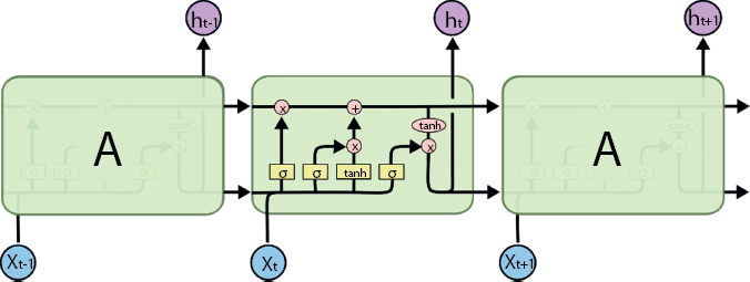
Figure 8.1 LSTM with four interacting layers.
This is considered as the sigmoid layer. It is taking the output at t − 1. The current input at the time t is also considered. After that it is combined into a tensor. The linear transformation along with a sigmoid is applied. Due to the sigmoid, the output of the gate lies between 0 and 1. The predicted value is then multiplied with the internal state. Because of this reason the state is named as forget gate. If ftgt = 0, then the previous internal state is entirely elapsed; whereas if ftgt = 1, then it can be agreed as not altered.
The input state takes the previous output composed with the new input and passes them through another sigmoid layer. This gate returns a value between 0 and 1. The value of the input gate is then multiplied with the output of the candidate layer.
Next, the layer applies hyperbolic tangent in association with the input and preceding output. This returns the candidate vector. The candidate vector is then added to the interior state, which is updated along with the given rule:
The previous gate is then multiplied by the forget gate, and also it is added to the fraction of the new candidate that is allowed by the output gate.
The gate controls what proportion of the interior state is accepted to the output and it works in a comparable means to the next gates. Figure 8.2 shows the loss incurred by the LSTM testing and training set. Here, we have used 30 epochs.
Let us have a look into Figure 8.2. As from the curve, we could see that the training loss is decreasing as the epochs are increasing, and after some time, they became constant which means our loss function is converged properly. In this process, the wind data has been taken and then the dataset is preprocessed. Then, the selective parameters like temperature, humidity, pressure, and wind speed are taken for processing and predicting the wind speed. Then, the input features are normalized. Now, we need to create the time series dataset looking back one time step. Then, 70% of data is utilized as the training data and 30% of data is utilized for testing purpose. We need to split them into inputs as well as output and then the input is reshaped to be 3D (samples, time steps, and features). The optimizer used for the process is Adam optimizer. We have used 44,071 total parameters for this process. The loss is calculated in each epoch.
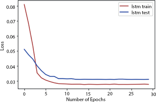
Figure 8.2 No. of epochs vs. loss.
Figure 8.3 shows the plotting amid the predicted test value and the real test value. The x axis consists of the time period and the y axis consists of the wind speed. Figure 8.4 shows the visualization over the full data.
Figure 8.5 is the plot over the small part of the data. Similarly, the plot over the very small part of the data is given in Figure 8.6.
In Figure 8.6, we can see that the actual and predicted pattern in the curve is almost similar which means that the algorithm is showing good results with less error.
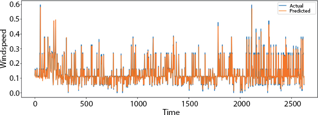
Figure 8.3 Actual and predicted test value.
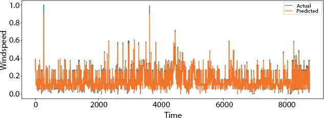
Figure 8.4 Visualization over full data.
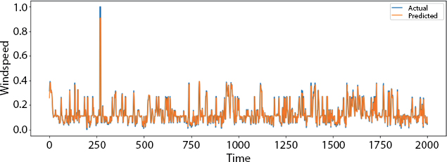
Figure 8.5 Plot over small part of the data.
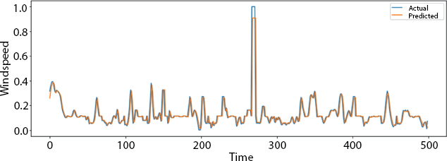
Figure 8.6 Plot over very small part of the data.
8.4 Gated Recurrent Unit
In general, RNNs have the problem of short-term memory. The RRNs suffer from vanishing gradient problem during the back propagation process. The gradients are the values which are used to apprise the neural network weights. The gradient shrinks during the vanishing gradient problem and the back propagation process is done by the time. When the gradient value becomes tremendously minor, it does not contribute much in learning.
nw stands for new weight, w stands for weight, lr stands for learning rate, and g stands for gradient. In RNN, the layers which get minor update break learning. These can be the previous layers. Due to the non-learning activity, it has the tendency to forget what are often perceived in longer sequences. Because of this, it has got a STM. GRU is one among the answer to STM and it is the interior mechanism called gates. These gates can regulate the flow of the data. The role of the gates here is that it can study the data within the sequence. This is the vital information used to decide whether to stay back or throw away. Due to this property, it is the potential of passing applicable evidence down the sequences with a long chain value. This is often helpful especially in doing certain predictions.
Figure 8.7 [22] shows the update gate and the reset gate. The forget gate and the update gate seems to be the same. The update gate acts almost like that of the input gate and forget gate of an LSTM. It decides on what information to throw away and what new information are often added. The reset gate is another gate and it is used to decide on what proportion past information has got to be forgotten. The GRUs are faster to train when compared with the LSTM. This is due to the fewer number of weights and parameters to update during training. In this process, the wind data has been taken and then the dataset is preprocessed. Then, the selective parameters like temperature, humidity, pressure, and wind speed are taken for processing and predicting the wind speed [12].
Then, the input features are normalized. Now, we need to create the time series dataset looking back one time step. Then, 70% of data is utilized as the training data and 30% of data is utilized for testing purpose. We need to split them into inputs as well as output and then the input is reshaped to be 3D (samples, time steps, and features). The optimizer used for the process is Adam optimizer. We have used 33,466 total parameters for this process. The loss is calculated in each epoch.
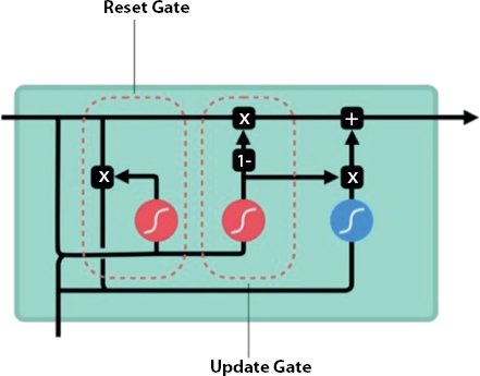
Figure 8.7 GRU.
Figure 8.8 shows the loss during each epoch. As from the curve, we could see that the training loss is decreasing as the epochs are increasing, and after some time, they became constant which means our loss function is converged properly. In the entire dataset, the number of epochs is a hyper parameter which describes the degree to which the learning algorithm will work through. So, one epoch is that each sample in the training dataset has got a chance to apprise the interior model parameters. The epoch is the combination of one or more than one batches.
Figure 8.9 shows the plotting among the foreseen test value and the actual test value. The x axis consists of the time period and the y axis consists of the wind speed. Figure 8.10 shows the visualization over the full data.
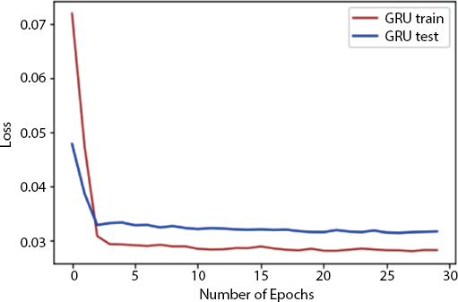
Figure 8.8 Number of epochs vs. loss.
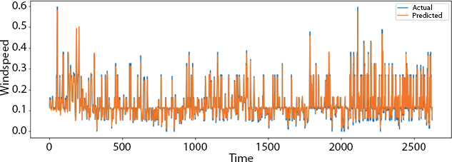
Figure 8.9 Plot of actual and predicted test value.
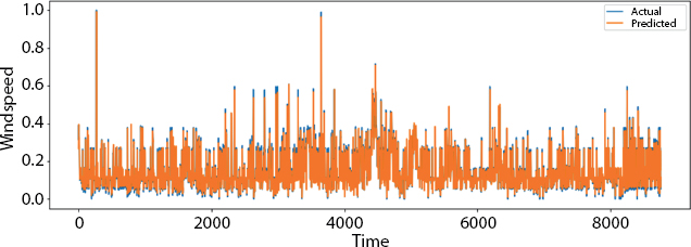
Figure 8.10 Visualization over full data.
The overall small part of the data for the actual and foreseen speed of the wind is shown in Figure 8.11.
Figure 8.12 shows the plot over the very small part of the data.
In Figure 8.12, we can see that the actual and predicted pattern in the curve is almost similar which means that the algorithm is showing good results with less error.
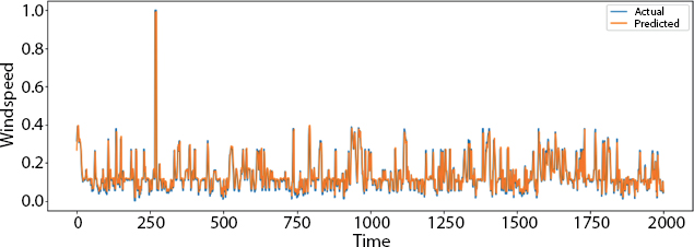
Figure 8.11 Plot over the small part of the data.
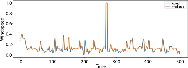
Figure 8.12 Plot over very small part of data.
8.5 Bidirectional Long Short-Term Memory Networks
The bidirectional RNNs puts two autonomous RNNs together. This structure permits the networks to possess both backward and forward information about the sequence at each time step. Using bidirectional will run the input in two ways: one from past to future and one from the future to past, and this varies the method from unidirectional is that within the LSTM that runs backward, and therefore, the information is preserved from the future and using the two hidden states has combined the information from both past and future are often preserved. The Bi-LSTM is shown in Figure 8.13 [23].
In this process, the wind data has been taken and then the dataset is preprocessed. Then, the selective parameters like temperature, humidity, pressure, and wind speed are taken for processing and predicting the wind speed. Then, the input features are normalized. Now, we need to create the time series dataset looking back one time step. Then, 70% of data is utilized as the training data and 30% of data is utilized for testing purpose. We need to split them into inputs as well as output and then the input is reshaped to be 3D (samples, time steps, and features). The optimizer used for the process is Adam optimizer. We have used 44,071 total parameters for this process. The loss is calculated in each epoch.
Figure 8.14 shows the loss during each epoch. As from the curve, we could see that the training loss is decreasing as the epochs are increasing, and after some time, they became constant which means our loss function is converged properly. Figure 8.15 shows the plotting among the forecast test value and the real test value. The x axis consists of the time period and the y axis consists of the wind speed. Figure 8.16 shows the visualization over the full data.
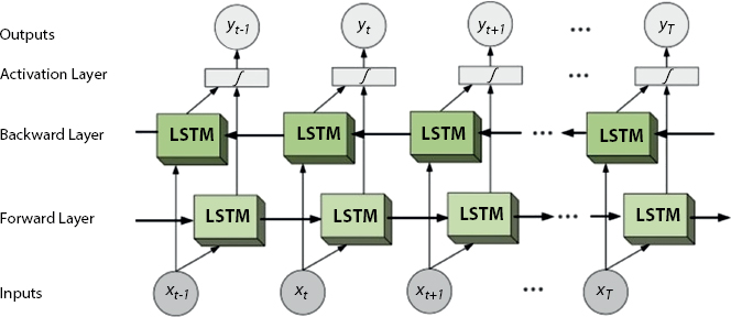
Figure 8.13 Bidirectional LSTM.
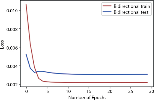
Figure 8.14 No. of epoch vs. loss.

Figure 8.15 Actual and predicted test value.

Figure 8.16 Visualization over full data.
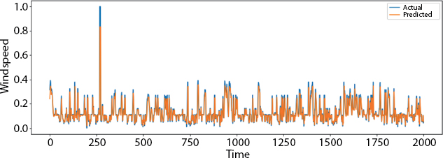
Figure 8.17 Plot over small part of the data.
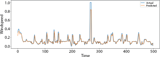
Figure 8.18 Plot over very small part of the data.
Figure 8.17 shows the plot over the small part of the data, and the plot over the very small part of data is shown in Figure 8.18.
In Figure 8.18, we can see that the actual and predicted pattern in the curve is almost similar which means that the algorithm is showing good results with less error.
8.6 Results and Discussion
The root mean square error (RMSE) is a strange key performance index, and it is also a very helpful parameter. It is well defined as the square root of the average squared error. RMSE can be considered as the square root of mean square error (MSE).
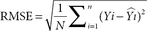
Table 8.1 Comparison of the methodologies with the parameters.
| Methodology | MSE | R-Squared | RMSE | MAE |
| LSTM | 0.003223 | 0.444921 | 0.056776 | 0.031272 |
| GRU | 0.003238 | 0.442399 | 0.056905 | 0.031254 |
| Bi-LSTM | 0.003027 | 0.478620 | 0.055026 | 0.031164 |
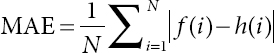
Table 8.1 comprises of the MSE, R-Squared, RMSE and MAE of the methodologies like LSTM, GRU and Bidirectional LSTM. The mean absolute error (MAE) characterizes the average of the absolute variance between the real and forecast values in the dataset. It measures the average of the residuals in the dataset.
MSE signifies the average of the squared difference between the original and the foreseen values in the dataset. It measures the variance of the residuals.
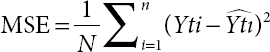
N can be considered as the number of data points, Yti is the observed values, and ![]() is the predicted values. The smaller the MSE, the closer we are to find the line of best fit. Initially, the difference between the Y and
is the predicted values. The smaller the MSE, the closer we are to find the line of best fit. Initially, the difference between the Y and ![]() for each available observation is taken, and then, the difference value is squared, and then, the sum squared values is found, and finally, it is divided by the total number of observations.
for each available observation is taken, and then, the difference value is squared, and then, the sum squared values is found, and finally, it is divided by the total number of observations.
8.7 Conclusion and Future Work
In this chapter, the deep learning methodologies like LSTM, GRU, and Bi-LSTM are used for extracting the chief trend content of the wind speed data. In comparing the performance of the algorithms, we can conclude the following results. Bi-LSTM is considered to be the good feature extractor, and it is followed by LSTM, GRU, and CNNLSTM. The coefficient of determination (R2), MSE, MAE, and RMSE has been computed for the given algorithms and the performance of the Bi-LSTM is comparatively good considering MSE, RMSE, and MAE.
In future, the quantity of the data related to wind speed would be considered. We will try to gather more data and thereby build more sensible replicas. New techniques based on deep learning can be deployed for getting better results. Automatic learning prediction models can also be used thereby learning the parameters which is consistent with the data.
References
1. Qureshi, A.S., Khan, A., Zameer, A., Usman, A., Wind power prediction using deep neural network based meta regression and transfer learning. Appl. Soft Comput., 58, 742–755, 2017.
2. Barbounis, T.G. and Theocharis, J.B., A locally recurrent fuzzy neural network with application to the wind speed prediction using spatial correlation. Neurocomputing, 70, 7–9, 1525–1542, 2007.
3. Bilgili, M. and Sahin, B., Comparative analysis of regression and artificial neural network models for wind speed prediction. Meteorol. Atmos. Phys., 109, 1, 61–72, 2010.
4. Cadenas, E. and Rivera, W., Wind speed forecasting in three different regions of Mexico, using a hybrid ARIMA–ANN model. Renewable Energy, 35, 12, 2732–2738, 2010.
5. Chang, G.W., Lu, H.J., Chang, Y.R., Lee, Y.D., An improved neural network-based approach for short-term wind speed and power forecast. Renewable Energy, 105, 301–311, 2017.
6. Ambach, D. and Schmid, W., A new high-dimensional time series approach for wind speed, wind direction and air pressure forecasting. Energy, 135, 833–850, 2017.
7. Damousis, I.G., Alexiadis, M.C., Theocharis, J.B., Dokopoulos, P.S., A fuzzy model for wind speed prediction and power generation in wind parks using spatial correlation. IEEE Trans. Energy Convers., 19, 2, 352–361, 2004.
8. Guo, Z., Zhao, W., Lu, H., Wang, J., Multi-step forecasting for wind speed using a modified EMD-based artificial neural network model. Renewable Energy, 37, 1, 241–249, 2012.
9. Liu, H., Chen, C., Tian, H.Q., Li, Y.F., A hybrid model for wind speed prediction using empirical mode decomposition and artificial neural networks. Renewable Energy, 48, 545–556, 2012.
10. Wang, J., Hu, J., Ma, K., Zhang, Y., A self-adaptive hybrid approach for wind speed forecasting. Renewable Energy, 78, 374–385, 2015.
11. JP, A., MapReduce and Optimized Deep Network for Rainfall Prediction in Agriculture. Comput. J., 63, 6, 900–912, 2020.
12. Kavasseri, R.G. and Seetharaman, K., Day-ahead wind speed forecasting using f-ARIMA models. Renewable Energy, 34, 5, 1388–1393, 2009.
13. Li, G. and Shi, J., On comparing three artificial neural networks for wind speed forecasting. Appl. Energy, 87, 7, 2313–2320, 2010.
14. Liu, H., Tian, H.Q., Chen, C., Li, Y.F., A hybrid statistical method to predict wind speed and wind power. Renewable Energy, 35, 8, 1857–1861, 2010.
15. Liu, H., Tian, H.Q., Li, Y.F., An EMD-recursive ARIMA method to predict wind speed for railway strong wind warning system. J. Wind Eng. Ind. Aerodyn., 141, 27–38, 2015.
16. Cai, H., Jia, X., Feng, J., Yang, Q., Hsu, Y.M., Chen, Y., Lee, J., A combined filtering strategy for short term and long term wind speed prediction with improved accuracy. Renewable Energy, 136, 1082–1090, 2019.
17. Yu, R., Gao, J., Yu, M., Lu, W., Xu, T., Zhao, M., Zhang, Z., LSTM-EFG for wind power forecasting based on sequential correlation features. Future Gener. Comput. Syst., 93, 33–42, 2019.
18. Cristin, R., Ananth, J.P., Raj, V.C., Illumination-based texture descriptor and fruitfly support vector neural network for image forgery detection in face images. IET Image Proc., 12, 8, 1439–1449, 2018.
19. Shi, J., Ding, Z., Lee, W.J., Yang, Y., Liu, Y., Zhang, M., Hybrid forecasting model for very-short term wind power forecasting based on grey relational analysis and wind speed distribution features. IEEE Trans. Smart Grid, 5, 1, 521–526, 2013.
20. Salcedo-Sanz, S., Perez-Bellido, A.M., Ortiz-García, E.G., Portilla-Figueras, A., Prieto, L., Paredes, D., Hybridizing the fifth generation mesoscale model with artificial neural networks for short-term wind speed prediction. Renewable Energy, 34, 6, 1451–1457, 2009.
21. https://colah.github.io/posts/2015-08-Understanding-LSTMs/
23. https://www.i2tutorials.com/deep-dive-into-bidirectional-lstm/
- *Corresponding author: [email protected]