
10
Forecasting of Electricity Consumption for G20 Members Using Various Machine Learning Techniques
Jaymin Suhagiya1, Deep Raval1*, Siddhi Vinayak Pandey2, Jeet Patel2, Ayushi Gupta3 and Akshay Srivastava3
1Department of Information and Communication Technology, Adani Institute of Infrastructure Engineering, Ahmedabad, Gujarat, India
2Department of Electrical Engineering, Adani Institute of Infrastructure Engineering, Ahmedabad, Gujarat, India
3Department of Electronics and Communication Engineering, Pranveer Singh Institute of Technology, Kanpur, Uttar Pradesh, India
Abstract
Forecasting the actual amount of electricity consumption with respect to demand of the load hasa always been a challenging task for each electricity generating station. In this manuscript, electricity consumption forecasting has been performed for G20 members. Recurrent Neural Networks, Linear Regression, Support Vector Regression, and Bayesian Ridge Regression have been used for forecasting, while sliding window approach has been used for the generation of the dataset. During experimentation, we have achieved Mean Absolute Error of 16.0714 TWh, R2 score of 0.9995, and Root Mean Squared Error of 31.3758 TWh with LSTM-based model trained on dataset created with window size of 6. Furthermore, predictions of electricity consumption have also been included till 2025.
Keywords: Electricity consumption, forecasting, machine learning, LSTM, GRU
10.1 Introduction
Electric consumption is the form of energy consumption that uses electric energy. On other words, electric consumption is the actual energy demand made on existing electricity supply. Various factors like weather, economic growth, and population affect the electricity consumption.
10.1.1 Why Electricity Consumption Forecasting Is Required?
Electricity consumption rate is reaching its peak and still being developmented using renewable and clean electricity resources is not globally practiced [1]. So, electricity demand management has become very important in the past few decades, and for same, people need to know how much electricity is consumed by any country in a particular time slot. Henceforth, electricity consumption forecasting is required to attain a balance in resources and electricity consumption [1]. Also, an unequivocal forecast helps various managers of electricity sector in various ways like setting up the future budgets and electricity consumption targets [2]. It also plays an important role in power industries as it helps to plan and make decisions on operation and working.
As the use of electricity is increasing day by day, the electricity consumption forecasting becomes important due to many reasons. One of the major reasons is that non-renewable sources are decreasing drastically, while the efficiency of renewable energy source is not a quite reliable in nature. Electricity consumption forecasting also helps during the power system expansion which starts from the future electricity consumption anticipations. If future increase of the load is needed, then cost and capacity of new power plant can be estimated. Electricity consumption forecasting can also be used for safety purpose. In industrial sector, the load consumed is peak load most of the time, but there is always a limit for a particular industry above which they cannot draw the power from the grid or else they are charged very heavy for the carelessness.
10.1.2 History and Advancement in Forecasting of Electricity Consumption
In 1880s, the power companies simply used Layman method for predicting the use of electricity in future. They predicted the future consumption by manually forecasting the future usage using charts, tables, and graphs [3]. Some factors of past methods like heating/cooling degree days, temperature-humidity index, and wind-chill factor are inherited by today’s consumption forecasting models.
In 1940s, when air conditioners were invented, the demand of electricity got tremendously affected by weather change and climate change. In winters, electricity usage got down, but in summers, it raised. After the discovery of air conditioners, there came electric heaters for winters. So, prediction and estimation of electricity consumption became very hectic by using the traditional method.
Presently, in this period of booming increment in innovation, demand of electricity has come to at apex [4, 5], so industrialists require a few progressed strategies for electricity consumption forecasting. There are created strategies like short-term, medium-term, and long-term electricity consumption forecasting [6, 7]. The long-term electricity consumption forecasting covers horizons of 1 to 10 years [8] and, in some cases, for various decades [9]. It confers month to month figure for top and valley in loads for different dissemination frameworks [10]. On the other hand, short-term load forecasting covers the variations from half an hour to few weeks [11].
10.1.3 Recurrent Neural Networks
Traditional feed forward neural networks cannot process the data of arbitrary length as their fundamental unit neuron does not support it. A recurrent cell is cell in which the output for the current timestep t (ot) depends on the previous hidden state (ht–1) of the cell. This makes recurrent cell suitable for the sequence-based tasks such as Speech Recognition, Natural Language Processing, and Forecasting, as now it can process input of any arbitrary length by iteratively updating its own hidden state which preserves some information from previous states. A neural networks containing recurrent cells instead of traditional neurons is known as Recurrent Neural Network (RNN). RNNs are mainly distinguished based on type of the cells used and their architecture. Figure 10.1 shows the basic RNN unrolled over t timesteps, where xt is input and ht is hidden state of the cell at timestep t.
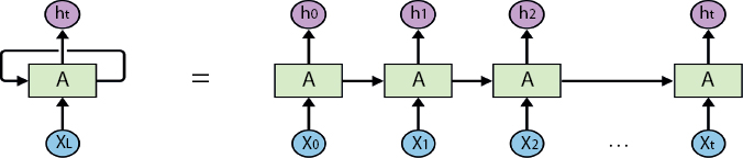
Figure 10.1 Traditional RNN unrolled over t timesteps [12].
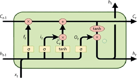
Figure 10.2 LSTM cell [16].
10.1.3.1 Long Short-Term Memory
Long Short-Term Memory (LSTM) was introduced by Hochreiter et al. [13] as a solution for the unstable (Vanishing/Expoding) gradients problem faced in traditional RNN. LSTM contains the additional “gates” which controls the flow of information in and out of the cell. Since the introduction of LSTM, there has been significant research aimed at improving it such as [14] and [15]. Although many variants of LSTM cell exist such as LSTM with a forget gate, LSTM without a forget gate and LSTM with a peep-hole connection, etc., the term LSTM generally refers to the LSTM with a forget gate. Figure 10.2 shows the internal structure of the LSTM cell. LSTM cell gets three inputs: previous cell state (Ct–1), previous hidden state (ht–1), and current input (xt) and gives three outputs: current cell state (Ct), current hidden state (ht), and current output (ot). LSTM cell contains three gates: forget gate (f), input gate (i), and output gate (o). Forget gate determines what information will be discarded from the previous state; this is controlled by the value of ft. Input gate determines which new information will be added to the cell state, and output gate determines the output based on the current cell state.
10.1.3.2 Gated Recurrent Unit
With LSTM being better and more sophisticated compared to traditional RNN, it also has the down side as it is computationally heavy. To address the same problem, Gated Recurrent Unit (GRU) was proposed by Cho et al. [17]. GRU contains only two gates, namely, a reset gate (r) and an update gate (z) which are the key factors in reducing and simplifying computation. Update gate combines the functionality of two gates of LSTM (forget gate and input gate) into one. Figure 10.3 shows the internal structure of typical GRU cell. GRU cell gets two inputs: previous hidden state (ht–1) and current input (xt) and gives only two outputs: current hidden state (ht) and current output (ot). GRU does not have the dedicated cell state as compared to LSTM’s cell state (Ct). Compared to LSTM, GRU struggles in the areas like context-free language and the cross-language translations [18, 19]. LSTM and GRU both are really solid candidates as a recurrent cell both of them perform similarly on many tasks.
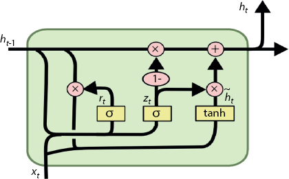
Figure 10.3 GRU cell [12].
10.1.3.3 Convolutional LSTM
To get the benefit of LSTM on spatiotemporal data, convolutional LSTM (ConvLSTM) was introduced leveraging power of both CNN (Convolutional Neural Network) and LSTM [20]. Figure 10.4 shows the structure of typical ConvLSTM cell. Internal structure of the cell is similar to LSTM cell as ConvLSTM uses LSTM internally. As ConvLSTM uses convolutional operator (*) instead of normal matrix multiplication (as used in LSTM). It preserves the spatial information from the data which is very helpful multidimensional data (like videos and audio). Even though ConvLSTM specializes in spatiotemporal data, it can also be also used on 1D data sequences by using appropriate kernel size.
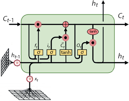
Figure 10.4 ConvLSTM cell.
10.1.3.4 Bidirectional Recurrent Neural Networks
Traditional RNN can only use the prior context to make predictions. Aimed at solving the same problem, Bidirectional RNN (BRNN) was proposed by Schuster et al. [21] which is simultaneously trained on the both time directions while using separate hidden layers for each time direction. Graves et al. [22] proposed the combination of both BRNN and LSTM, namely, Bidirectional LSTM. Training is similar to a regular RNN as two layers do not interact with each other directly their outputs are only concatenated. Figure 10.5 shows the demonstration of a typical BRNN.
10.1.4 Other Regression Techniques
Linear Regression is one of the most simple regression techniques. Linear Regression typically try to generalize the function of type f(x) = m · x + b on given data, where x is an input, m is a slope, and b is a bias. Optimization techniques (such as Gradient Descent) are used to get the optimal values of m and b such that error function (like MSE and MAE) is minimum.

Figure 10.5 Bidirectional RNN.
Linear regression can be further extended for multiple inputs, more formally for n inputs: f(x1, x2,…, xn) = m1 · x1 + m2 · x2 + · + mn · xn + b.
Support Vector Regression (SVR) creates a system in which data is trained from series of examples in accordance to successfully predict the output. It is a type of supervised learning. A SVR model is formed by using kernels sparse matrix and solutions, Vapnik-Chervonenkis control model, and support vectors [23]. In SVR, symmetrical loss function is used for training the datasets. Binary classification problems can be solved using SVR models by formulating them as convex optimization problems [23].
Bayesian Ridge Regression is a regression model with parameter estimation method where parameter is estimated by multiplying posterior distribution with prior distribution. In linear regression model using OLS estimation method, the error as well as variables are normally distributed. The Bayesian approach can be done by using MCMC (Markov Chain Monte Carlo) algorithm [24]. To estimate the efficiency of linear model by Bayesian regression, Theil’s Coefficient is used, which is a statistical technique that predicts the efficiency by calculating the difference between original value and the predicted value.
10.2 Dataset Preparation
The dataset utilized in this paper is prepared by Enerdata organization [25]. The dataset originally contains yearly electricity domestic consumption (in TWh) for 61 entities (including countries, continents, and unions) for the years 1990 to 2019. This paper focuses on G20 members, which includes Argentina, Australia, Brazil, Canada, China, France, Germany, India, Indonesia, Italy, Japan, South Korea, Mexico, Russia, Saudi Arabia, South Africa, Turkey, United Kingdom, United States, and European Union. Among all G20 members, 19 are the countries and one is the European Union.
The raw dataset is the time-series dataset as it gives us the electricty consumption data on regular interval (i.e., year). To tackle the forecasting of the future years as a supervised learning problem, we created the new data-set from the original one using sliding window approach. In each sample, N timesteps are given and the model should the (N + 1)th timestep, where N is the window size. In other words, previous N years will be input to the model and (N + 1)th year will be the label. For example, in the case of window size 4, previous 4 years’ electricity consumption is given and next year is there as a label. This way model can learn trend from previous timesteps and make appropriate prediction for the next timestep. This approach can give us the large amount of training data compared to raw training data at the cost of data repetition. Figure 10.6 shows the demonstration of sliding window on the time-series data. Window sizes 1 and 2 will not be enough for learning trend, and on the other hand, window sizes greater than 7 would just make dataset much smaller. Hence, we created five seprate data-sets with window sizes 3–7 keeping the data of the years 2016–2019 for testing purpose. Table 10.1 shows the number of training and testing samples in all datasets created using different window sizes.
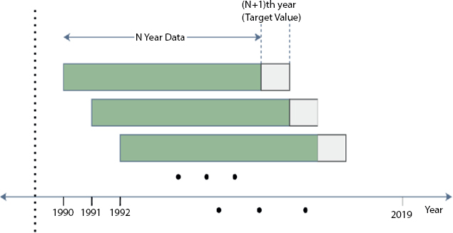
Figure 10.6 Demonstration of the sliding window approach.
Table 10.1 Training and test size for generated dataset from each window size.
| Window size | Training samples | Testing samples |
| 3 | 460 | 80 |
| 4 | 440 | 80 |
| 5 | 420 | 80 |
| 6 | 400 | 80 |
| 7 | 380 | 80 |
10.3 Results and Discussions
All the experiments have been performed in Python using TensorFlow and ScikitLearn libraries. Computational specifications of machine utilized during experimentation are Ryzen 5 4600H, NVIDEA GTX 1650 4GB, and 8 GB DDR4 Ram.
Table 10.2 Performance of all trained models.
| Cell type | Window size | R2 score | MAE | RMSE |
| LSTM | 3 | 0.998749625 | 21.44645568 | 52.01252557 |
| 4 | 0.999258582 | 19.49052397 | 40.05153819 | |
| 5 | 0.999271694 | 20.73799729 | 39.69580909 | |
| 6 | 0.999544997 | 16.07145371 | 31.37582087 | |
| 7 | 0.999216397 | 19.84262385 | 41.17519839 | |
| GRU | 3 | 0.999352065 | 19.44009694 | 37.44153438 |
| 4 | 0.99943614 | 18.98304995 | 34.9279822 | |
| 5 | 0.999360785 | 19.37603302 | 37.18873189 | |
| 6 | 0.999435172 | 18.08372996 | 34.95793729 | |
| 7 | 0.999324213 | 19.17705701 | 38.23779332 | |
| Biodirectional LSTM | 3 | 0.998901652 | 20.68070089 | 48.74811593 |
| 4 | 0.998855535 | 20.34128753 | 49.76098863 | |
| 5 | 0.999180335 | 19.30442693 | 42.11201091 | |
| 6 | 0.999426774 | 17.55318267 | 35.21685526 | |
| 7 | 0.999206407 | 20.02302547 | 41.43683245 | |
| ConvLSTM | 3 | 0.999091009 | 19.33748763 | 44.34734645 |
| 4 | 0.999277166 | 19.27017771 | 39.54640382 | |
| 5 | 0.999234165 | 19.86183365 | 40.70571966 | |
| 6 | 0.99948358 | 17.51624149 | 33.42638218 | |
| 7 | 0.999426936 | 18.16709740 | 35.21189519 | |
| Support Vector Regression | 3 | 0.999397458 | 18.54912241 | 36.10615607 |
| 4 | 0.999470774 | 18.75444142 | 33.83827126 | |
| 5 | 0.999218605 | 22.26829334 | 41.11714657 | |
| 6 | 0.999059587 | 24.65530079 | 45.10731731 | |
| 7 | 0.998177736 | 28.27401743 | 62.79041968 | |
| Linear Regression | 3 | 0.999493775 | 18.78475962 | 33.09475573 |
| 4 | 0.999239879 | 21.56018059 | 40.55356501 | |
| 5 | 0.999243397 | 22.45643728 | 40.45961526 | |
| 6 | 0.999091294 | 24.85775704 | 44.34036331 | |
| 7 | 0.998655929 | 26.14611200 | 53.92607458 | |
| Bayesian Ridge Regression | 3 | 0.999506349 | 18.69629528 | 32.68115425 |
| 4 | 0.999253988 | 21.22020898 | 40.17541841 | |
| 5 | 0.999124103 | 22.34981485 | 43.53255683 | |
| 6 | 0.999025962 | 24.57856065 | 45.90665126 | |
| 7 | 0.998969954 | 24.72536657 | 47.20803097 |
We experimented with LSTM, GRU, Bidirectional LSTM, ConvLSTM, Linear Regression, SVR, and Bayesian Ridge Regression. Models based on LSTM, GRU, and Bidirectional LSTM have two recurrent layers stacked followed by a dense layer. Each recurrent layer has 36 units, while the last layer has only 1 unit. First two layers have ReLU as an activation function, while the last has linear activation function which simply gives the activation values without applying any additional computation. ConvLSTM-based model has similar architecture except; it has 64 filters in first two layers followed by the flatten layer which flattens the previous layer’s output, so it can be fed to the last dense layer. All of the recurrent models were trained for the maximum of 200 epochs with Adam [26] as an optimizer (having the slow learning rate of 1e–3) and huber (which is less sensitive to outliers compared to Mean Squared Error) as the objective function. Grid search was used (to search for the best parameters) in Linear Regression, SVR, and Bayesian Ridge Regression. SVR was performed with the linear kernel. All of the models were trained on four different datasets. Table 10.2 performance of all the models on test data in terms of R2 score, Mean Absolute Error (in TWh), and Root Mean Squared Error (in TWh).
Seeing the test error rates, it can be concluded that we get the best performance for window size = 6 while using the LSTM-based model. Ignoring the best model, these are not far away in terms of the test error rates. However, performance of Linear Regression, SVR, and Bayesian Ridge Regression is slightly worse than that of recurrent models. Furthermore, in our experiments, we have found regression techniques tend to over estimate the values of future by large margin because of the same reason, we have used only recurrent models for forecasting. Figure 10.7 shows the actual predictions of the different recurrent models (trained with window size = 6) for the all G20 members. Before the vertical line, all model’s performance can be compared to the ground truth at particular timestep (i.e.. year). After the vertical line, up to the year 2025, all models try to predict next values independently of each other. Years where previous true values are not available, model is self-fed its own predicted values. Although this carries the error forward, we can get a rough estimate of the next values models that would actually predict if they were given true values. Table 10.3 analyzes predictions further by comparing the demand in 2019 with the predicted demand in 2025.
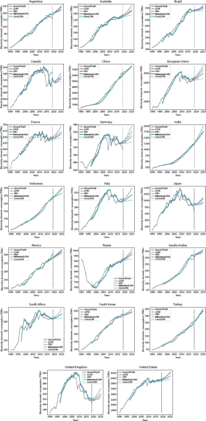
Figure 10.7 Predictions done by models trained with window size = 6.
Table 10.3 Statistical analysis of the prediction done by LSTM model (widow size = 6).
| Member | 2019 (TWh) | 2025 (TWh) | Absolute difference (TWh) | Percentage difference (%) | Individual mean absolute error (TWh) |
| Argentina | 124.802 | 156.596 | 31.794 | 25.476 | 6.53 |
| Australia | 234.977 | 250.202 | 15.225 | 6.4792 | 0.734 |
| Brazil | 536.047 | 547.57 | 11.523 | 2.1496 | 8.882 |
| Canada | 542.986 | 523.695 | –19.291 | –3.553 | 15.257 |
| China | 6510.22 | 7570.87 | 1060.6 | 16.292 | 80.19 |
| France | 436.556 | 462.671 | 26.135 | 5.9866 | 5.707 |
| Germany | 516.801 | 549.677 | 32.876 | 6.3614 | 5.423 |
| India | 1230.35 | 1774.14 | 543.79 | 44.198 | 29.926 |
| Indonesia | 245.308 | 298.302 | 52.994 | 21.603 | 2.648 |
| Italy | 300.614 | 314.38 | 13.766 | 4.5793 | 3.997 |
| Japan | 918.219 | 987.93 | 69.712 | 7.592 | 18.98 |
| South Korea | 553.414 | 589.763 | 36.348 | 6.568 | 11.722 |
| Mexico | 307.31 | 323.838 | 16.528 | 5.3784 | 5.24 |
| Russia | 922.277 | 964.14 | 41.863 | 4.5391 | 6.084 |
| Saudi Arabia | 288.784 | 353.749 | 68.965 | 23.881 | 19.638 |
| South Africa | 203.651 | 216.293 | 12.642 | 6.2078 | 1.85 |
| Turkey | 254.486 | 349.566 | 95.08 | 37.362 | 8.678 |
| United Kingdom | 302.716 | 315.553 | 12.837 | 4.2407 | 2.432 |
| United States | 3865.06 | 4085.8 | 220.74 | 5.7111 | 53.528 |
| European | 2850.4 | 2999.73 | 149.33 | 5.2389 | 33.976 |
| Total | 21144.98 | 23638.49 | 2493.51 | 11.81 (Average) | 16.0715 (Average) |
10.4 Conclusion
Forecasting electricity consumption for G20 members has been performed using various machine learning techniques. The best recurrent model was able to achieve MAE of 16.0714 TWh, R2 score of 0.9995, and RMSE of 31.3758 TWh, while the best regression techinque achieved MAE of 18.549 TWh, R2 score of 0.9994, and RMSE of 36.106 TWh. As RNNs are better at handling longer sequences, they perform well with window size of 6, while other regression techniques perform well on window size of 3. Taking into consideration forecasting done by recurrent models, it can be concluded that total electricity demand of all G20 countries (excluding European Union) combined can increase anywhere from 1,957.35 TWh to 2,549.67 TWh in upcoming 5 years. Furthermore, countries like Argentina, India, Indonesia, Saudi Arabia, and Turkey can see rapid increase in electricity demand, while India being at top with 44.198%.
Acknowledgement
The authors would like to thank Enerdata Organization for allowing us to use the Domestic Energy Consumption Data prepared by them and cooperating with us in the completion of this chapter.
References
1. Ghalehkhondabi, I., Ardjmand, E., Weckman, G.R., Young, W.A., An overview of energy demand forecasting methods published in 2005–2015. Energy Syst., 8, 2, 411–447, 2017.
2. Amber, K.P., Aslam, M.W., Hussain, S.K., Electricity consumption forecasting models for administration buildings of the uk higher education sector. Energy Build., 90, 127–136, 2015.
3. Hong, T., Gui, M., Baran, M.E., Willis, H.L., Modeling and forecasting hourly electric load by multiple linear regression with interactions, in: IEEE PES General Meeting, pp. 1–8, 2010.
4. Wang, Z., Li, J., Zhu, S., Zhao, J., Deng, S., Shengyuan, Z., Yin, H., Li, H., Qi, Y., Gan, Z., A review of load forecasting of the distributed energy system. IOP Conference Series: Earth and Environmental Science, 03 2019, vol. 237, p. 042019.
5. Alagbe, V., Popoola, S.I., Atayero, A.A., Adebisi, B., Abolade, R.O., Misra, S., Artificial intelligence techniques for electrical load forecasting in smart and connected communities, in: International Conference on Computational Science and Its Applications, Springer, pp. 219–230, 2019.
6. Scott, D., Simpson, T., Dervilis, N., Rogers, T., Worden, K., Machine learning for energy load forecasting. J. Phys.: Conf. Ser., 1106, 012005, 10 2018.
7. Xiao, L., Shao, W., Liang, T., Wang, C., A combined model based on multiple seasonal patterns and modified firefly algorithm for electrical load forecasting. Appl. Energy, 167, 135–153, 2016.
8. Baliyan, A., Gaurav, K., Mishra, S.K., A review of short term load forecasting using artificial neural network models. Proc. Comput. Sci., 48, 121–125, 2015.
9. Esteves, G.R.T., Bastos, B.Q., Cyrino, F.L., Calili, R.F., Souza, R.C., Long term electricity forecast: a systematic review. Proc. Comput. Sci., 55, 549–558, 2015.
10. Daneshi, H., Shahidehpour, M., Choobbari, A.L., Long-term load forecasting in electricity market, in: 2008 IEEE International Conference on Electro/Information Technology, IEEE, pp. 395–400, 2008.
11. Jacob, M., Neves, C., Greetham, D.V., Short Term Load Forecasting, pp. 15–37, Springer International Publishing, Cham, 2020.
12. Understanding lstm networks, colah’s blog. https://colah.github.io/posts/2015-08-Understanding-LSTMs/, United States, 2020, [Online; accessed 01-October-2020].
13. Hochreiter, S. and Schmidhuber, J., Long short-term memory. Neural Comput., 9, 1735–80, 12 1997.
14. Gers, F.A. and Schmidhuber, J., Recurrent nets that time and count, in: Proceedings of the IEEE-INNS-ENNS International Joint Conference on Neural Networks. IJCNN 2000. Neural Computing: New Challenges and Perspectives for the New Millennium, vol. 3, IEEE, pp. 189–194, 2000.
15. Gers, F., Long short-term memory in recurrent neural networks, Doctoral dissertation, Verlag nicht ermittelbar, 2001.
16. Varsamopoulos, S., Bertels, K., Almudever, C.G., Comparing neural network based decoders for the surface code. IEEE Trans. Comput., 69, 2, 300–311, 2019.
17. Cho, K., Van Merriënboer, B., Gulcehre, C., Bahdanau, D., Bougares, F., Schwenk, H., Bengio, Y., Learning phrase representations using rnn encoder-decoder for statistical machine translation, computation and language: machine learning. arXiv preprint arXiv:1406.1078, 1–15, 2014.
18. Weiss, G., Goldberg, Y., Yahav, E., On the practical computational power of finite precision rnns for language recognition, 1–9, 2018. https://arxiv.org/abs/1805.04908
19. Britz, D., Le, Q., Pryzant, R., Effective domain mixing for neural machine translation. In Proceedings of the Second Conference on Machine Translation, pp. 118–126, 2017.
20. Xingjian, S., Chen, Z., Wang, H., Yeung, D.-Y., Wong, W.-K., Woo, W.-c., Convolutional lstm network: A machine learning approach for precipitation nowcasting, in: Advances in neural information processing systems, pp. 802–810, 2015.
21. Schuster, M. and Paliwal, K.K., Bidirectional recurrent neural networks. IEEE Trans. Signal Process., 45, 11, 2673–2681, 1997.
22. Graves, A. and Schmidhuber, J., Framewise phoneme classification with bidirectional lstm and other neural network architectures. Neural Networks, 18, 5–6, 602–610, 2005.
23. Awad, M. and Khanna, R., Support Vector Regression, pp. 67–80, Apress, Berkeley, CA, 2015.
24. Permai, S.D. and Tanty, H., Linear regression model using bayesian approach for energy performance of residential building. Proc. Comput. Sci., 135, 671–677, 2018, The 3rd International Conference on Computer Science and Computational Intelligence (ICCSCI 2018): Empowering Smart Technology in Digital Era for a Better Life.
25. World Power consumption, Electricity consumption, Enerdata, https://yearbook.enerdata.net/electricity/electricity-domestic-consumption-data.html, Grenole - France, 2020, [Online; accessed 01-October-2020].
26. Kingma, D.P. and Ba, J., A method for stochastic optimization. Anon. International Conference on Learning Representations, SanDiago ICLR, pp. 22–31, 2015.
- *Corresponding author: [email protected]