
Uncertainty Quantification in Internet of Battlefield Things
Brian Jalaian; Stephen Russell US Army Research Laboratory, Adelphi, MD, United States
Abstract
Internet of Things (IoT) technologies have made considerable recent advances in commercial applications, prompting new research on their use in military applications. The Internet of Battlefield Things (IoBT) is the military counterpart of IoT, which is capable of leveraging mixed commercial and military technologies. Machine learning and artificial intelligence are the fundamental algorithmic building blocks of IoBT to address the decision-making problems that arise in underlying control, communication, and networking within the IoBT infrastructure in addition to the inevitable part of almost all military-specific applications developed over IoBT. Uncertainty quantification for machine learning and artificial intelligence within IoBT is critical to provide an accurate measure of error over the output in addition to precision of output. Such information on uncertainty quantification enables risk-aware decision making and control for subsequent intelligent systems and/or humans within the IoBT pipeline. This chapter provides an overview of classical and modern statistical-learning theory, and how numerical optimization can be used to solve the corresponding mathematical problems with an emphasis on uncertainty quantification.
Keywords
Internet of Battle Things; Intelligent systems; Decision making
2.1 Introduction
The battlefield of the future will comprise a vast array of heterogeneous computational capable sensors, actuators, devices, information sources, analytics, humans, and infrastructure, with varying intelligence, capabilities, and constraints on energy, power, computing, and communication resources. To maintain information dominance, the future army must far surpass the ability of future opposing forces, kinetic and nonkinetic alike, to ensure mission success and minimize risks. This vision can only be achieved if systems progress from a state of total dependence on human control to autonomous and, ultimately, autonomic behavior. A highly adaptive and autonomous future will depend upon foundational algorithms, theories, and methods that do not fully exist today. There are many challenges in ensuring that the delegated mission goals are accomplished regardless of the immediate availability of human presence in the control loop or the partial attrition of mission assets.
During the past decade, there has been a tremendous growth in the field of machine learning (ML). Large datasets combined with complex algorithms, such as deep neural networks, have allowed for huge advances across a variety of disciplines. However, despite the success of these models there has not been as much focus on uncertainty quantification (UQ); that is, quantifying a model's confidence in its predictions. In some situations, UQ may not be a huge priority (e.g., Netflix recommending movie titles). But in situations where the wrong prediction is a matter of life or death, UQ is crucial. For instance, if army personnel in combat are using an ML algorithm to make decisions, it is vital to know how confident the given algorithm is in its predictions. Personnel may observe a data point in the field that is quite different from the data the algorithm was trained on, yet the algorithm will just supply a (likely poor) prediction, potentially resulting in a catastrophe.
In this chapter we first provide a background and motivation scenario in Section 2.2. In Section 2.4, we discuss how to be able to quantify and minimize the uncertainty with respect to training an ML algorithm. This leads us to the field of stochastic optimization, which is covered broadly in this section. In Section 2.4, we discuss UQ in ML. Specifically, we study how to develop ways for a model to know what it doesn’t know. In other words we study how to enable the model to be especially cautious for data that is different from that on which it was trained. Section 2.5 explores the recent emerging trends on adversarial learning, which is a new application of UQ in ML in Internet of Battlefield Things (IoBT) in an offensive and defensive capacity. Section 2.6 concludes the chapter.
2.2 Background and Motivating IoBT Scenario
In recent years the Internet of Things (IoT) technologies have seen significant commercial adoption. For IoT technology, a key objective is to deliver intelligent services capable of performing both analytics and reasoning over data streams from heterogeneous device collections. In commercial settings IoT data processing has commonly been handled through cloud-based services, managed through centralized servers and high-reliability network infrastructures.
Recent advances in IoT technology have motivated the defense community to research IoT architecture development for tactical environments, advancing the development of the IoBT for use in C4ISR applications (Kott, Swami, & West, 2016). Toward advancing IoBT adoption, differences in military versus commercial network infrastructures become an important consideration. For many commercial IoT architectures, cloud-based services are used to perform needed data processing, which rely upon both stable network coverage and connectivity. As observed in Zheng and Carter (2015), IoT adoption in the tactical environment faces several technical challenges: (i) limitations on tactical network connectivity and reliability, which impact the amount of data that can be obtained from IoT sensor collections in real time; (ii) limitations on interoperability between IoT infrastructure components, resulting in reduced infrastructure functionality; and (iii) availability of data analytics components accessible over tactical network connections, capable of real-time data ingest over potentially sparse IoT data collections.
Challenges such as these limit the viability of cloud-based service usage in IoBT infrastructures. Hence, significant changes to existing commercial IoT architectures become necessary to ensure their applicability, particularly in the context of ML applications. To help illustrate these challenges, a motivating scenario is provided.
2.2.1 Detecting Vehicle-Borne IEDs in Urban Environments
As part of an ongoing counterinsurgency operation by coalition forces in the country of Aragon, focus is placed on monitoring of insurgent movements and activities. Vehicle-borne improvised explosive devices (VBIEDs) have become more frequently used by insurgents in recent months, requiring methods for quick detection and interception. Recent intelligence reports have provided details on the physical appearance of IED-outfitted vehicles in the area. However, due to the time constraints in confirming detections of VBIEDs, methods for autonomous detection become desirable. To support VBIED detection, an IoBT infrastructure has been deployed by coalition forces consisting of a mix of unattended ground sensors (UGSs) and unmanned aerial systems (UASs). In turn, supervised learning methods are employed over sensor data gathered from both sources.
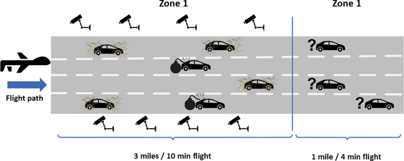
Recent intelligence has indicated that VBIEDs may be used in a city square during the annual Aragonian Independence Festival. A local custom for this festival involves decoration of vehicles with varying articles (including flags and Christmas tree lighting). A UAS drone is tasked with patrolling the airspace over one of the inbound roadways and recoding images of detected vehicles. However, due to the decorations present on many civilian vehicles, confidence in VBIED classification by the UAS is significantly reduced. To mitigate this, the drone flies along a 3-mile stretch of road for 10 minutes to gather new images of the decorated vehicles. In each case the drone generates a classification of each vehicle as VBIED or not, each with a particular confidence value. For low-confidence readings, the drone contacts a corresponding UGS to do the following: (i) take a high-resolution image, and (ii) take readings for presence of explosives-related chemicals in the air nearby, where any detectable explosives confirms the vehicle is a VBIED. Since battery power for the UGS is limited, along with available network bandwidth, the UAS should only request UGS readings when especially necessary. Following receipt of data from a UGS, the UAS performs retraining of the classifier to improve the accuracy of future VBIED classification attempts. Over a short period, the UAS has gathered additional training data to support detection of VBIEDs. Eventually, the drone passes over a 1-mile stretch of road lacking UGSs. At this point the UAS must classify detected vehicles without UGS support (Fig. 2.1).
This example scenario highlights several research issues specific to IoBT settings, as reflected in prior surveys (e.g., Suri et al., 2016; Zheng & Carter, 2015): (i) a needed capability to quickly gather training data reflecting unforeseen learning/classification tasks; (ii) a needed capability to incrementally learn over the stream of field-specific data (e.g., increasing the accuracy of classifying VBIEDs by learning over the stream of pictures of decorated cars collected over 10 minutes of flight time); and (iii) management of limited network bandwidth and connectivity between assets (e.g., between the UAS and UGS along the road) requiring selective asset use to obtain classifier-relevant data that increases the classifier knowledge.
Each of these issues requires the selection of learning and classification methods appropriate to stream-based data sources. Prior research (Bottou, 1998 b; Bottou & Cun, 2004; Vapnik, 2013) demonstrates the equivalence of learning from stream-based data in real time with learning from infinite samples. From this work it follows that statistical-learning methods adept to large-scale data sources may be applicable for stream-based data.
This chapter opens with a survey of classical and modern statistical-learning theory, and how numerical optimization can be used to solve the resulting mathematical problems. The objective of this chapter is to encourage the IoT and ML research communities to revisit the underlying mathematical underpinnings of stream-based learning, as they apply to IoBT-based systems.
2.3 Optimization in Machine Learning
Behind the scenes of any ML algorithm is an optimization problem. To maximize a likelihood or a posterior distribution, or minimize a loss function, one must rely on mathematical optimization.
Of course the optimization literature provides numerous algorithms including gradient descent, Newton's method, Quasi-Newton methods, and nonlinear CG. In many applications these methods have been widely used for some time with much success. However, the size of contemporary datasets as well as complex model structure make traditional optimization algorithms ill suited for contemporary ML problems. For example, consider the standard gradient descent algorithm. When the objective function is strongly convex, the training uncertainty (or training error), f(xk) − f(x⁎), is proportional to en−k, where n is the amount of training data and k is the number of iterations of the algorithm. Thus the training uncertainty grows exponentially with the size of the data. For large datasets, gradient descent clearly becomes impractical.
Stochastic gradient descent (SGD), on the other hand, has training uncertainty proportional to 1/k. Although this error decreases more slowly in terms of k, it is independent of the sample size, giving it a clear advantage in a modern settings. Moreover, in a stochastic optimization setting, SGD actually achieves the optimal complexity rate in terms of k. These two features, as well as SGD's simplicity, have allowed it to become the standard optimization algorithm for most large-scale ML problems, such as training neural nets. However, SGD is not without its drawbacks. In particular, it performs poorly for badly scaled problems (when the Hessian is ill conditioned) and can have high variance with its step directions. While SGD's performance starts off particularly strong, its convergence to the optimum quickly slows. Although no stochastic algorithm can do better than SGD in terms of error uncertainty (in terms of k), there is certainly potential to improve the convergence rate up to a constant factor.
With regard to uncertainty, we would like to achieve a sufficiently small error for our model as quickly as possible. In the next section we discuss the formal stochastic optimization problem, the standard SGD algorithm, along with two popular variants of SGD. In Section 2.3 we propose an avenue for the development of an SGD variant that seems especially promising and discuss avenues of research for UQ in model predictions.
2.3.1 Optimization Problem
The standard stochastic optimization problem is:
where expectation is taken with respect to the probability distribution of ξ = (X, Y), the explanatory, and response variables. In ML, F(w;ξ) is typically of the form:
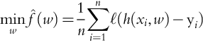
where ℓ is some loss function, such as ∥⋅∥2. Most optimization algorithms attempt to optimize what is called the sample-path problem, the solution of which is often referred to as the empirical risk minimizer (ERM). This strategy attempts to solve an approximation to f(w) using a finite amount of training data:
This is the problem that the bulk of ML algorithms attempt to minimize. A particular instance is maximum likelihood estimation, perhaps the most widely used estimation method among statisticians. For computer scientists minimizing a loss function (such as ℓ2 loss) without an explicit statistical model is more common.
Although it may go without saying that minimizing ![]() is not the end goal. Ideally we wish to minimize the true objective, f(w). For finite sample sizes one runs into issues of overfitting to the sample problem. An adequate solution to the sample problem may not generalize well to future predictions (especially true for highly complex, over-parameterized models). Some ways of combating this problem include early-stopping, regularization, and Bayesian methods. In a large data setting, however, we can work around this issue. Due to such large sample sizes, we have an essentially infinite amount of data. Additionally, we are often in an online setting where data are continuously incoming, and we would like our model to continuously learn from new data. In this case we can model data as coming from an oracle that draws from the true probability distribution Pξ (such a scheme is fairly standard among the stochastic optimization community, but is more rare in ML). In this manner we can optimize the true risk (1) with respect to the objective function, f(w).
is not the end goal. Ideally we wish to minimize the true objective, f(w). For finite sample sizes one runs into issues of overfitting to the sample problem. An adequate solution to the sample problem may not generalize well to future predictions (especially true for highly complex, over-parameterized models). Some ways of combating this problem include early-stopping, regularization, and Bayesian methods. In a large data setting, however, we can work around this issue. Due to such large sample sizes, we have an essentially infinite amount of data. Additionally, we are often in an online setting where data are continuously incoming, and we would like our model to continuously learn from new data. In this case we can model data as coming from an oracle that draws from the true probability distribution Pξ (such a scheme is fairly standard among the stochastic optimization community, but is more rare in ML). In this manner we can optimize the true risk (1) with respect to the objective function, f(w).
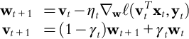
2.3.2 Stochastic Gradient Descent Algorithm
Algorithm 2.1 shows a generic SGD algorithm to be used to solve (1). The direction of each iteration, g(xk, ξk) depends on the current iterate xk as well as a random draw ξi ∼ Pξ.
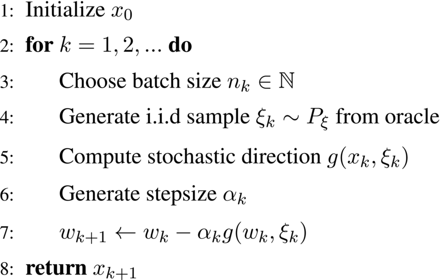
The basic SGD algorithm sets nk = 1, ![]() and computes the stochastic direction as:
and computes the stochastic direction as:
This is essentially the full-gradient method only evaluated for one sample point. Using the standard full-gradient method would require n gradient evaluations every iteration, but the basic SGD algorithm only requires the evaluation of one. We briefly discuss an implementation for logistic regression.
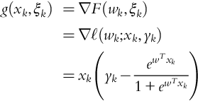
2.3.3 Example: Logistic Regression
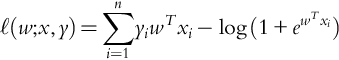
To make this algorithm more concrete, consider the case of binary logistic regression. When the amount of data is manageable, a standard way (Hastie, Tibshirani, & Friedman, 2009) to find the optimal parameters is to apply Newton's method (since there is no closed-form solution) to the log-likelihood for the model:
However, when n is large, this quickly becomes unfeasible. Instead, we could use a simple SGD implementation. In this case we set the stochastic direction to be a random gradient evaluated at ξk = (Xk, Yk), which is sampled from the oracle:
The implemented algorithm is then (Algorithm 2.2):
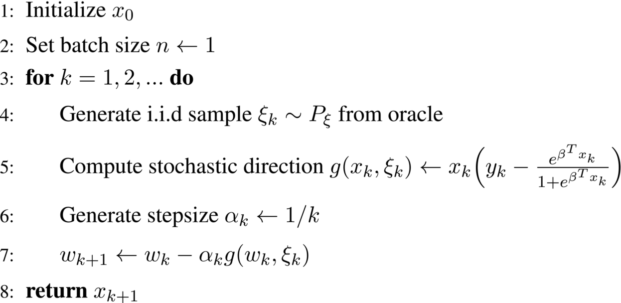
Again, note that for each iteration only a single training point is evaluated. On the other hand the full-gradient method would have to use the entire dataset for every iteration.
2.3.4 SGD Variants
As mentioned in Section 2.1, the basic SGD algorithm has some room for improvement. In this section we introduce two popular SGD variants: mini-batch SGD and SGD with momentum. Each variant gives a different yet useful way of improving upon the basic SGD algorithm.
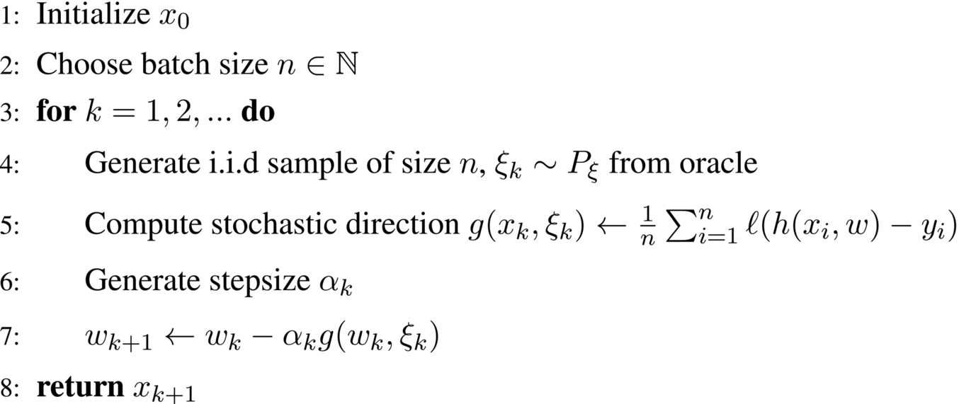
2.3.4.1 Mini-Batch SGD
One of the major issues with SGD is that its search directions have high variance. Instead of moving downhill as intended, the algorithm may wander around randomly more than we would like. A natural idea is to use a larger sample size for the gradient estimates. The basic SGD uses a sample size of n = 1, so it makes sense that we might wish to use more draws from the oracle to reduce the variance. Specifically, we would reduce the variance in gradient estimates by a factor of ![]() , where n is the batch size. The mini-batch algorithm is implemented as shown in Algorithm 2.3.
, where n is the batch size. The mini-batch algorithm is implemented as shown in Algorithm 2.3.
It is shown in Bottou, Curtis, and Nocedal (2016) that under assumptions of smoothness and strong convexity, standard SGD (sample size n = 1 with fixed α) achieves an error rate of:

This convergence rate has several assumption-dependent constants such as the Lipschitz constant L and strong-convexity parameter c. However, the defining feature of that algorithm is the (⋅)k−1 term, which implies that the error decreases exponentially to the constant ![]() . Using mini-batch SGD, on the other hand, yields the following bound:
. Using mini-batch SGD, on the other hand, yields the following bound:

Thus the mini-batch algorithm converges at the same rate, but to a smaller error constant. This is certainly an improvement in terms of the error bound, but of course requires n − 1 more samples at each iteration than the standard SGD. Thus it is not entirely clear which algorithm is better. If one could perform mini-batch in parallel with little overhead cost, the resulting algorithm would achieve the described bound without the cost of sampling n draws sequentially. Otherwise, the tradeoff is somewhat ambiguous.
2.3.4.2 SGD With Momentum
Another issue with standard SGD is that it does not take into account scaling of the parameter space (which would require second-order information). A particular situation where this is an issue is when the objective function has very narrow level curves. Here, a standard gradient descent method tends to zigzag back and forth, moving almost perpendicular to the optimum. A common solution in the deterministic case is to use gradient descent with momentum, which has a simple yet helpful addition to the descent step. The stochastic version is:
where the last term is the momentum term.
As the name implies, this algorithm is motivated by the physical idea of the inertia, for example, of a ball rolling down a hill. It might make sense to incorporate the previous step length this way into the next search direction. In this sense, the algorithm “remembers” all previous step distances, in the form of an exponentially decaying average. Momentum helps SGD avoid getting stuck in narrow valleys and is popular for training neural networks. Unfortunately, convergence for momentum is not as well understood. An upper bound for a convex, nonsmooth objective is given by Yang, Lin, and Li (2016) in the form of:
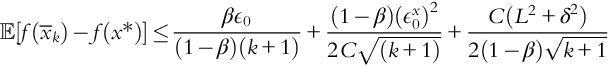
Note here that the error is given in terms of the average of the iterate ![]() . For problems in this class the optimal convergence rate is
. For problems in this class the optimal convergence rate is ![]() , which this algorithm achieves.
, which this algorithm achieves.
2.3.5 Nesterov's Accelerated Gradient Descent
Nesterov's accelerated gradient descent (NAGD) algorithm for deterministic settings has been shown to be optimal for a variety of problem assumptions. For example, in the case where the objective is smooth and strongly convex, NAGD achieves the lower complexity bound, unlike standard gradient descent (Nesterov, 2004). Currently, there has not been a lot of attention given to NAGD in the stochastic setting (though, see Yang et al., 2016). We would like to extend NAGD to several problem settings in a stochastic context. Additionally, we would like to incorporate adaptive sampling (using varying batch sizes) into a stochastic NAGD. Adaptive sampling has shown promise, yet has not received a lot of attention.
The development of a more-efficient SGD algorithm would reduce uncertainty in the training of ML models at a faster rate than current algorithms. This is especially important for online learning, where it is crucial that algorithms adapt efficiently to newly observed data in the field.
2.3.6 Generalized Linear Models
The first and simplest choice of estimator function class is ![]() . In this case, the estimator is a generalized linear model (GLM):
. In this case, the estimator is a generalized linear model (GLM): ![]() for some parameter vector
for some parameter vector ![]() (Nelder & Baker, 1972). In this case optimizing the statistical loss is the stochastic convex optimization problem, stated as:
(Nelder & Baker, 1972). In this case optimizing the statistical loss is the stochastic convex optimization problem, stated as:
Observe that to optimize Eq. (2.3), assuming a closed-form solution is unavailable, a gradient descent or Newton's method must be used (Boyd & Vanderberghe, 2004). However, either method requires computing the gradient of ![]() , which requires infinitely many realizations (xn, yn) of the random pair (x, y), and thus has infinite complexity. This computational bottleneck has been resolved through the development of stochastic approximation (SA) methods (Bottou, 1998 a; Robbins & Monro, 1951), which operate on subsets of data examples per step. The most common SA method is the SGD, which involves descending along the stochastic gradient ∇wℓ(wTxt, yt) rather than the true gradient at each step:
, which requires infinitely many realizations (xn, yn) of the random pair (x, y), and thus has infinite complexity. This computational bottleneck has been resolved through the development of stochastic approximation (SA) methods (Bottou, 1998 a; Robbins & Monro, 1951), which operate on subsets of data examples per step. The most common SA method is the SGD, which involves descending along the stochastic gradient ∇wℓ(wTxt, yt) rather than the true gradient at each step:
Use of SGD (Eq. 2.4) is prevalent due to its simplicity, ease of use, and the fact that it converges to the minimizer of Eq. (2.3) almost certainly, and in expectation at a ![]() rate when L(w) is convex and a sublinearly
rate when L(w) is convex and a sublinearly ![]() when it is strongly convex. Efforts to improve the mean convergence rate to
when it is strongly convex. Efforts to improve the mean convergence rate to ![]() through the use of Nesterov acceleration (Nemirovski, Juditsky, Lan, & Shapiro, 2009) have also been developed, whose updates are given as:
through the use of Nesterov acceleration (Nemirovski, Juditsky, Lan, & Shapiro, 2009) have also been developed, whose updates are given as:
A plethora of tools have been proposed specifically to minimize the empirical risk (sample size N is finite) in the case of GLMs, which achieve even faster linear or superlinear convergence rates. These methods are either based on reducing the variance of the SA (data-subsampling) error of the stochastic gradient (Defazio, Bach, & Lacoste-Julien, 2014; Johnson & Zhang, 2013; Schmidt, Roux, & Bach, 2013) or by using approximate second-order (Hessian) information (Goldfarb, 1970; Shanno & Phua, 1976). This thread has culminated in the fact that quasi-Newton methods (Mokhtari, Gürbüzbalaban, & Ribeiro, 2016) outperform variance reduction methods (Hu, Pan, & Kwok, 2009) for finite-sum minimization when N is large scale. For specifics on stochastic quasi-Newton updates, see Mokhtari and Ribeiro (2015) and Byrd, Hansen, Nocedal, and Singer (2016). However, as ![]() , the analysis that yields linear or superlinear learning rates breaks down, and the best one can hope for is Nesterov's
, the analysis that yields linear or superlinear learning rates breaks down, and the best one can hope for is Nesterov's ![]() rate (Nemirovski et al., 2009).
rate (Nemirovski et al., 2009).
2.3.7 Learning Feature Representations for Inference
Transformations of data domains have become widely used in the past decades, due to their ability to extract useful information from input signals as a precursor to solving statistical inference problems. For instance, if the signal dimension is very large, dimensionality reduction is of interest, which may be approached with principal component analysis (Jolliffe, 1986). If instead one would like to conduct multiresolution analysis, wavelets (Mallat, 2008) may be more appropriate. These techniques, which also include a k-nearest neighbor, are known as unsupervised or signal representation learning (Murphy, 2012). Recently, methods based on learned representations, rather than those fixed a priori, have gained traction in pattern recognition (Elad & Aharon, 2006; Mairal, Elad, & Sapiro, 2008). A special case of data-driven representation learning is dictionary learning (Mairal, Bach, Ponce, Sapiro, & Zisserman, 2008), the focus of this section.
Here we address finding a dictionary (signal encoding) that is well adapted to a specific inference task (Mairal, Bach, & Ponce, 2012). To do so, denote the coding ![]() as a feature representation of the signal xt with respect to some dictionary matrix
as a feature representation of the signal xt with respect to some dictionary matrix ![]() . Typically,
. Typically, ![]() is chosen as the solution to a lasso regression or approximate solution to an ℓ0 constrained problem that minimizes some criterion of distance between DTα and x to incentivize codes to be sparse. Further introduce the classifier
is chosen as the solution to a lasso regression or approximate solution to an ℓ0 constrained problem that minimizes some criterion of distance between DTα and x to incentivize codes to be sparse. Further introduce the classifier ![]() that is used to predict target variable yt when given the signal encoding
that is used to predict target variable yt when given the signal encoding ![]() . The merit of the classifier
. The merit of the classifier ![]() is measured by the smooth loss function
is measured by the smooth loss function ![]() that captures how well the classifier w may predict yt when given the coding
that captures how well the classifier w may predict yt when given the coding ![]() . Note that α is computed using the dictionary
. Note that α is computed using the dictionary ![]() . The task-driven dictionary learning problem is formulated as the joint determination of the dictionary
. The task-driven dictionary learning problem is formulated as the joint determination of the dictionary ![]() and classifier
and classifier ![]() that minimize the cost
that minimize the cost ![]() averaged over the training set:
averaged over the training set:
In Eq. (2.6) we specify the estimator ![]() , which parameterizes the function class
, which parameterizes the function class ![]() as the product set
as the product set ![]() . For a given dictionary
. For a given dictionary ![]() and signal sample xt, we compute the code
and signal sample xt, we compute the code ![]() as per some lasso regression problem, for instance, and then predict yt using w, and measure the prediction error with the loss function
as per some lasso regression problem, for instance, and then predict yt using w, and measure the prediction error with the loss function ![]() . The optimal pair
. The optimal pair ![]() in Eq. (2.6) is the one that minimizes the cost averaged over the given sample pairs (xt, yt). Observe that
in Eq. (2.6) is the one that minimizes the cost averaged over the given sample pairs (xt, yt). Observe that ![]() is not a variable in the optimization in Eq. (2.6) but a mapping for an implicit dependence of the loss on the dictionary
is not a variable in the optimization in Eq. (2.6) but a mapping for an implicit dependence of the loss on the dictionary ![]() . The optimization problem in Eq. (2.6) is not assumed to be convex—this would be restrictive because the dependence of ℓ on
. The optimization problem in Eq. (2.6) is not assumed to be convex—this would be restrictive because the dependence of ℓ on ![]() is, partly, through the mapping
is, partly, through the mapping ![]() defined by some sparse-coding procedure. In general, only local minima of Eq. (2.6) can be found. This formulation has, nonetheless, been successful in solving practical pattern recognition tasks in vision (Mairal et al., 2012) and robotics (Koppel, Fink, Warnell, Stump, & Ribeiro, 2016).
defined by some sparse-coding procedure. In general, only local minima of Eq. (2.6) can be found. This formulation has, nonetheless, been successful in solving practical pattern recognition tasks in vision (Mairal et al., 2012) and robotics (Koppel, Fink, Warnell, Stump, & Ribeiro, 2016).
The lack of convexity of Eq. (2.6) means that attaining statistical consistency for supervised dictionary learning methods is much more challenging than for GLMs. To this end, the prevalence of nonconvex stochastic programs arising from statistical learning based on nonlinear transformations of the feature space ![]() has led to a renewed interest in nonconvex optimization methods through applying convex techniques to nonconvex settings (Boyd & Vanderberghe, 2004). This constitutes a form of simulated annealing (Bertsimas & Tsitsiklis, 1993) with successive convex approximation (Facchinei, Scutari, & Sagratella, 2015). A compelling achievement of this recent surge is the hybrid convex-annealing approach, which has been shown to be capable of finding a global minimizer (Raginsky, Rakhlin, & Telgarsky, 2017). However, the use of these methods for addressing the training of estimators defined by nonconvex stochastic programs requires far more training examples to obtain convergence than convex problems and requires further demonstration in practice.
has led to a renewed interest in nonconvex optimization methods through applying convex techniques to nonconvex settings (Boyd & Vanderberghe, 2004). This constitutes a form of simulated annealing (Bertsimas & Tsitsiklis, 1993) with successive convex approximation (Facchinei, Scutari, & Sagratella, 2015). A compelling achievement of this recent surge is the hybrid convex-annealing approach, which has been shown to be capable of finding a global minimizer (Raginsky, Rakhlin, & Telgarsky, 2017). However, the use of these methods for addressing the training of estimators defined by nonconvex stochastic programs requires far more training examples to obtain convergence than convex problems and requires further demonstration in practice.
2.4 Uncertainty Quantification in Machine Learning
Most standard ML algorithms only give a single output: the predicted value ![]() . While this is a primary goal of ML, as discussed in Section 2.1, it is important in many scenarios to also have a measure of model confidence. In particular, we would like the model to take into account variability due to new observations being “far” from the data on which the model was trained. This is particularly interesting for tactical application in which the human decision makers rely on the confidence of the predictive model to make actionable decisions. Unfortunately, this area has not been widely developed. We explore two ways of UQ in the context of ML: explicit and implicit uncertainty measures.
. While this is a primary goal of ML, as discussed in Section 2.1, it is important in many scenarios to also have a measure of model confidence. In particular, we would like the model to take into account variability due to new observations being “far” from the data on which the model was trained. This is particularly interesting for tactical application in which the human decision makers rely on the confidence of the predictive model to make actionable decisions. Unfortunately, this area has not been widely developed. We explore two ways of UQ in the context of ML: explicit and implicit uncertainty measures.
By explicit measures we mean methods that, in addition to a model's prediction ![]() , perform a separate computation to determine the model's confidence in that particular point. These methods often measure some kind of distance between a new data point and the training data. New data that are far away from the training data give reason to proceed with caution. A naive way to measure confidence explicitly would be to output an indicator variable that tells whether the new data points fall within the convex hull of the training data. If a point does not fall within the convex hull, the user would have reason to be suspicious of that prediction. More complicated methods can be applied using modern outlier detection theory (model-based methods, proximity-based methods, etc.). In particular, these methods can give more indicative measures of confidence, as opposed to a simple 1 or 0, and are more robust to outliers within the training data.
, perform a separate computation to determine the model's confidence in that particular point. These methods often measure some kind of distance between a new data point and the training data. New data that are far away from the training data give reason to proceed with caution. A naive way to measure confidence explicitly would be to output an indicator variable that tells whether the new data points fall within the convex hull of the training data. If a point does not fall within the convex hull, the user would have reason to be suspicious of that prediction. More complicated methods can be applied using modern outlier detection theory (model-based methods, proximity-based methods, etc.). In particular, these methods can give more indicative measures of confidence, as opposed to a simple 1 or 0, and are more robust to outliers within the training data.
Another approach to UQ is incorporating the uncertainty arising from new data points in the ML model implicitly. A natural way of doing this is using a Bayesian approach: we can use a Gaussian process (GP) to model our beliefs about the function that we wish to learn. Predictions have a large variance in regions where little data has been observed, and smaller variance in regions where the observed data are more dense. However, for large, high-dimensional datasets, GPs become difficult to fit. Current methods that approximate GPs in some way that show promise include variational inference methods, dropout neural networks (Das, Roy, & Sambasivan, 2017), and neural network ensembles (Lakshminarayanan, Pritzel, & Blundell, 2017).
We explore the above techniques for UQ in intelligent battlefield systems. We believe that the development of ways to measure UQ could be of great use in areas that use ML or artificial intelligence to make risk-informed decisions, particularly when poor predictions come with a high cost.
2.4.1 Gaussian Process Regression
Gaussian process regression (GPR) is a framework for nonlinear, nonparametric, Bayesian inference (Rasmussen, 2004) (kriging; Krige, 1951). GPR is widely used in chemical processing (Kocijan, 2016), robotics (Deisenroth, Fox, & Rasmussen, 2015), and ML (Rasmussen, 2004), among other applications. One of the main drawbacks of GPR is its complexity, which scales cubically N3 with the training sample size N in batch setting.
GPR models the relationship between random variables ![]() and
and ![]() , that is,
, that is, ![]() by function f(x), which should be estimated upon the basis of N training examples
by function f(x), which should be estimated upon the basis of N training examples ![]() . Unlike in ERM, GPR does not learn this estimator by solving an optimization problem that assesses the quality of its fitness, but instead assumes that this function f(x) follows some particular parameterized family of distributions, in which the parameters need to be estimated (Krige, 1951; Rasmussen, 2004).
. Unlike in ERM, GPR does not learn this estimator by solving an optimization problem that assesses the quality of its fitness, but instead assumes that this function f(x) follows some particular parameterized family of distributions, in which the parameters need to be estimated (Krige, 1951; Rasmussen, 2004).
In particular, for GPs, a uniform prior on the distribution of ![]() is placed as a Gaussian distribution, namely,
is placed as a Gaussian distribution, namely, ![]() . Here
. Here ![]() denotes the multivariate Gaussian distribution in N dimensions with mean vector
denotes the multivariate Gaussian distribution in N dimensions with mean vector ![]() and covariance
and covariance ![]() . In GPR, the covariance
. In GPR, the covariance ![]() is constructed from a distance-like kernel function
is constructed from a distance-like kernel function ![]() defined over the product set of the feature space. The kernel expresses some prior about how to measure distance between points, a common example of which is itself the Gaussian,
defined over the product set of the feature space. The kernel expresses some prior about how to measure distance between points, a common example of which is itself the Gaussian, ![]() with bandwidth hyperparameter c.
with bandwidth hyperparameter c.
In standard GPR, a Gaussian prior on the noise will be placed that corrupts ![]() to form the observation vector y = [y1, …, yN], that is,
to form the observation vector y = [y1, …, yN], that is, ![]() where σ2 is some variance parameter. The prior can be integrated on
where σ2 is some variance parameter. The prior can be integrated on ![]() to obtain the marginal likelihood for y as:
to obtain the marginal likelihood for y as:
Upon receiving a new data point xN+1, a Bayesian inference ![]() can be made, not by simply setting a point estimate
can be made, not by simply setting a point estimate ![]() . Instead, the entire posterior distribution can be formulated for yN+1 as:
. Instead, the entire posterior distribution can be formulated for yN+1 as:
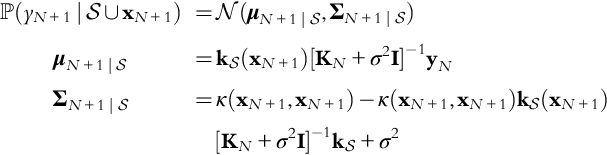
While this approach to sequential Bayesian inference provides a powerful framework for fitting a mean and covariance envelope around observed data, it requires for each N the computation of ![]() and
and ![]() , which crucially depend on computing the inverse of the kernel matrix KN every time a new data point arrives. It is well known that matrix inversion has cubic complexity
, which crucially depend on computing the inverse of the kernel matrix KN every time a new data point arrives. It is well known that matrix inversion has cubic complexity ![]() in the variable dimension N, which may be reduced through use of Cholesky factorization (Foster et al., 2009) or subspace projections (Banerjee, Dunson, & Tokdar, 2012) combined with various compression criteria such as information gain (Seeger, Williams, & Lawrence, 2003), mean square error (Smola & Bartlett, 2001), integral approximation for Nyström sampling (Williams & Seeger, 2001), probabilistic criteria (Bauer, van der Wilk, & Rasmussen, 2016; McIntire, Ratner, & Ermon, 2016), and many others (Bui, Nguyen, & Turner, 2017).
in the variable dimension N, which may be reduced through use of Cholesky factorization (Foster et al., 2009) or subspace projections (Banerjee, Dunson, & Tokdar, 2012) combined with various compression criteria such as information gain (Seeger, Williams, & Lawrence, 2003), mean square error (Smola & Bartlett, 2001), integral approximation for Nyström sampling (Williams & Seeger, 2001), probabilistic criteria (Bauer, van der Wilk, & Rasmussen, 2016; McIntire, Ratner, & Ermon, 2016), and many others (Bui, Nguyen, & Turner, 2017).
2.4.2 Neural Network
While the mathematical formulation of convolutional neural networks and their variants have been around for decades (Haykin, 1998), their use has only become widespread in recent years as computing power and data pervasiveness has made them not impossible to train. Since the landmark work (Krizhevsky, Sutskever, & Hinton, 2012) demonstrated their ability to solve image recognition tasks on much larger scales than previously addressable, they have permeated many fields, such as speech (Graves, Mohamed, & Hinton, 2013), text (Jaderberg, Simonyan, Vedaldi, & Zisserman, 2016), and control (Lillicrap et al., 2015). An estimator function class ![]() can be defined by the composition of many functions of the form gk(x) =wkσk(x). σk is a nonlinear “activation function,” which can be, for example, a rectified linear unit
can be defined by the composition of many functions of the form gk(x) =wkσk(x). σk is a nonlinear “activation function,” which can be, for example, a rectified linear unit ![]() , a sigmoid σk(a) = 1/(1 + ea), or a hyperbolic tangent σk(a) = (1 − e−2a)/(1 + e−2a). Specifically, for a K-layer convolutional neural network, the estimator is given as:
, a sigmoid σk(a) = 1/(1 + ea), or a hyperbolic tangent σk(a) = (1 − e−2a)/(1 + e−2a). Specifically, for a K-layer convolutional neural network, the estimator is given as:
and typically one tries to make the distance between the target variable and the estimator small by minimizing their quadratic distance:
where each wk is a vector whose length depends on the number of “neurons” at each layer of the network. This operation may be thought of as an iterated generalization of a convolutional filter. Additional complexities can be added at each layer, such as aggregating values output for the activation functions by their maximum (max pooling) or average. But the training procedure is similar: minimize a variant of the highly nonconvex, high-dimensional stochastic program (Eq. 2.10). Due to their high dimensionality, efforts to modify nonconvex stochastic optimization algorithms to be amenable to parallel computing architectures have gained salience in recent years. An active area of research is the interplay between parallel stochastic algorithms and scientific computing to minimize the clock time required for training neural networks—see Lian, Huang, Li, and Liu (2015), Mokhtari, Koppel, Scutari, and Ribeiro (2017), and Scardapane and Di Lorenzo (2017). Thus far, efforts have been restricted to attaining computational speedup by parallelization to convergence at a stationary point, although some preliminary efforts to escape saddle points and ensure convergence to a local minimizer have also recently appeared (Lee, Simchowitz, Jordan, & Recht, 2016); these modify convex optimization techniques, for instance, by replacing indefinite Hessians with positive definite approximate Hessians (Paternain, Mokhtari, & Ribeiro, 2017).
2.4.3 Uncertainty Quantification in Deep Neural Network
In this section we discuss UQ in neural networks through Bayesian methods, more specifically, posterior sampling. Hamiltonian Monte Carlo (HMC) is the best current approach to perform posterior sampling in neural networks. HMC is the foundation from which all other existing approaches are derived. HMC is an MCMC method (Brooks, Gelman, Jones, & Meng, 2011) that has been a popular tool in the ML literature to sample from complex probability distributions when random walk-based first-order Langevin samplers do not exhibit the desired convergence behaviors. Standard HMC approaches are designed to propose candidate samplers for a Metropolis-Hastings-based acceptance scheme with high acceptance probabilities; since calculation of these M-H ratios necessitates a pass through the entire dataset, scalability of HMC-based algorithms has been limited. This has been addressed recently with the development of stochastic approaches, inspired by the now ubiquitous SGD-based ERM algorithms, where we omit the M-H correction step and calculate the Hamiltonian gradients over random mini-batches of the training data (Chen, Fox, & Guestrin, 2014; Welling & Teh, 2011). Further improvements to these approaches have been done by incorporating Riemann manifold techniques to learn the critically important Hamiltonian mass matrices, both in the standard HMC (Girolami & Calderhead, 2011) and stochastic (Ma, Chen, & Fox, 2015; Roychowdhury, Kulis, & Parthasarathy, 2016) settings. These Riemannian approaches have been shown to noticeably improve the acceptance probabilities of samples following the methods of those proposed by Girolami and Calderhead (2011), and dramatically improve the convergence rates in the stochastic formulations as well (Roychowdhury et al., 2016).
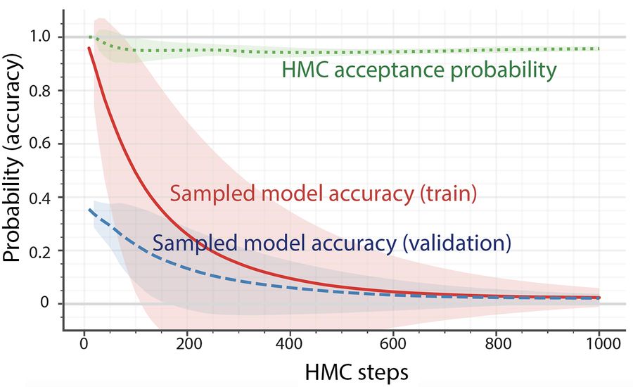
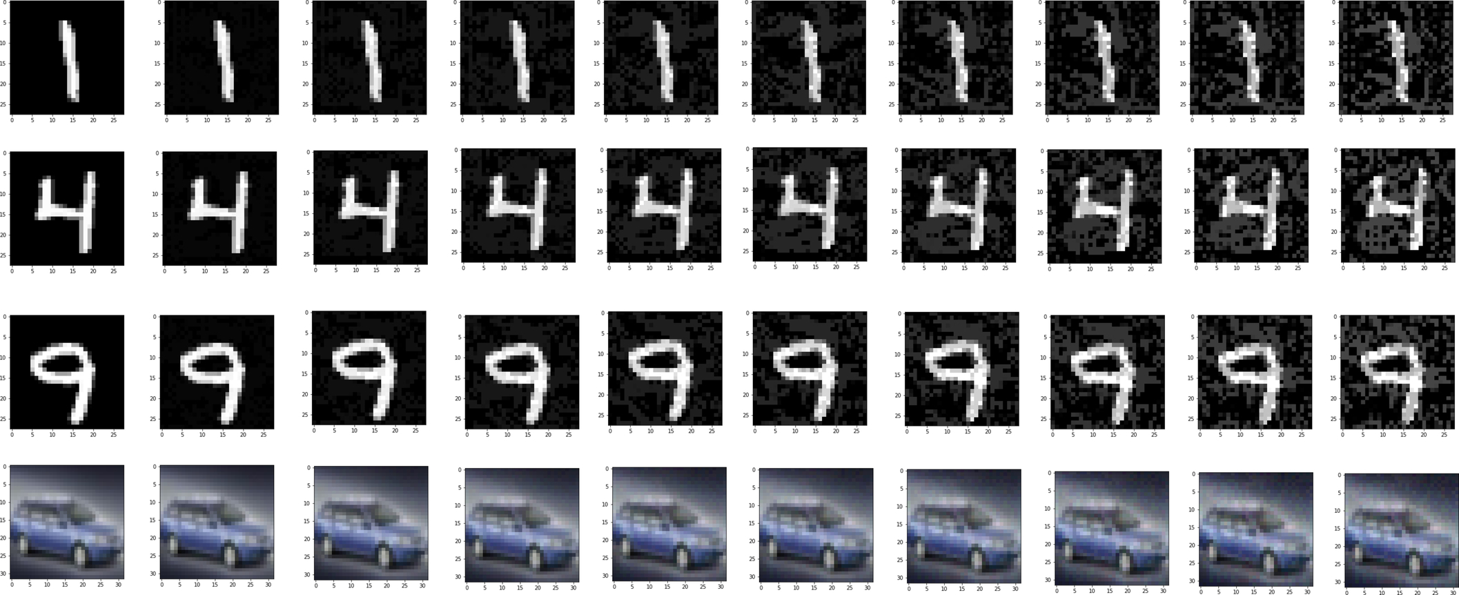
Preliminary experiments show that HMC does not work well in practice. Thus one can identify two challenges with posterior sampling using HMC. First, HMC still has a hard time finding the different modes of the distribution (i.e., if it can escape metastable regions of the HMC Markov chain). Second, as stated earlier, the massive dimensionality of deep neural networks make the most of the posterior probability mass that resides in models with poor classification accuracy. Fig. 2.2 shows sampled neural network models as a function of HMC steps for CIFAR100 image classification task (using a LeNet CNN architecture). In as few as 100 HMC steps, the posterior-sampled models are significantly worse than the best models in both training and validation accuracies. Thus HMC posterior sampling is impractical for deep neural networks, even as the HMC acceptance probability is high throughout the experiment.
It is an open avenue of research to explore a few mode exploration fixes. Here, traditional MCMC methods can be used, such as annealing and annealing importance sampling. Less traditional methods are also explored, such as stochastic initialization and model perturbation.
Regarding the important challenge of posterior sampling accurate models in an given posterior mode, mini-batch stochastic gradient Langevin dynamics (SGLD) (Welling & Teh, 2011) is increasingly credited to being a practical Bayesian method to train neural networks to find good generalization regions (Chaudhari et al., 2017), and it may help in improving parallel SGD algorithms (Chaudhari et al., 2017). The connection between SGLD and SGD has been explored in Mandt, Hoffman, and Blei (2017) for posterior sampling in small regions around a locally optimal solution. To make this procedure a legitimate posterior sampling approach, we explore the use of Chaudhari et al.’s (2017) methods to smooth out local minima and significantly extend the reach of Mandt et al.’s (2017) posterior sampling approach.
This smoothing out has connections to Riemannian curvature methods to explore the energy function in the parameter (weight) space (Poole, Lahiri, Raghu, Sohl-Dickstein, & Ganguli, 2016). The Hessian, which is a diffusion curvature, is used by Fawzi, Moosavi-Dezfooli, Frossard, and Soatto (2017) as a measure of curvature to empirically explore the energy function of learned model with regard to examples (the curvature with regard to the input space, rather than the parameter space). This approach is also related to the implicit regularization arguments of Neyshabur, Tomioka, Salakhutdinov, and Srebro (2017).
There is a need to develop an alternative SGD-type method for accurate posterior sampling of deep neural network models that is capable of giving the all-important UQ in the decision-making problem in C3I systems. Not surprisingly a system that correctly quantifies the probability that a suggested decision is incorrect inspires more confidence than a system that incorrectly believes itself to always be correct; the latter is a common ailment in deep neural networks. Moreover, a general practical Bayesian neural network method would help provide robustness against adversarial attacks (as the attacker needs to attack a family of models, rather than a single model), reduce generalization error via posterior-sampled ensembles, and provide better quantification of classification accuracy and root mean square error (RMSE).
2.5 Adversarial Learning in DNN
Unfortunately these models have been shown to be very brittle and vulnerable to specially crafted adversarial perturbations to examples: given an input x and any target classification t, it is possible to find a new input x′ that is similar to x but classified as t. These adversarial examples often appear almost indistinguishable from natural data to human perception and are, as yet, incorrectly classified by the neural network. Recent results have shown that accuracy of neural networks can be reduced from close to 100% to below 5% using adversarial examples. This creates a significant challenge in deploying these deep learning models in security-critical domains where adversarial activity is intrinsic, such as IoBT, cyber networks, and surveillance. The use of neural networks in computer vision and speech recognition has brought these models into the center of security-critical systems where authentication depends on these machine-learned models. How do we ensure that adversaries in these domains do not exploit the limitations of ML models to go undetected or trigger an unintended outcome?
Multiple methods have been proposed in literature to generate adversarial examples as well as defend against adversarial examples. Adversarial example-generation methods include both white-box and black-box attacks on neural networks (Goodfellow, Shlens, & Szegedy, 2014; Papernot et al., 2017; Papernot, McDaniel, Jha, et al., 2016; Szegedy et al., 2013), targeting feed-forward classification networks (Carlini & Wagner, 2016), generative networks (Kos, Fischer, & Song, 2017), and recurrent neural networks (Papernot, McDaniel, Swami, & Harang, 2016). These methods leverage gradient-based optimization for normal examples to discover perturbations that lead to misprediction—the techniques differ in defining the neighborhood in which perturbation is permitted and the loss function used to guide the search. For example, one of the earliest attacks (Goodfellow et al., 2014) used a fast sign gradient method (FGMS) that looks for a similar image x′ in the ![]() neighborhood of x. Given a loss function Loss(x, l) specifying the cost of classifying the point x as label l, the adversarial example x′ is calculated as:
neighborhood of x. Given a loss function Loss(x, l) specifying the cost of classifying the point x as label l, the adversarial example x′ is calculated as:
FGMS was improved to an iterative gradient sign approach (IGSM) in Kurakin, Goodfellow, and Bengio (2016) by using a finer iterative optimization strategy, where the attack performs FGMS with a smaller step-width α and clips the updated result so that the image stays within the ϵ boundary of x. In this approach, the ith iteration computes the following:
In contrast to FGSM and IGSM, DeepFool (Moosavi-Dezfooli, Fawzi, & Frossard, 2016) attempts to find a perturbed image x′ from a normal image x by finding the closest decision boundary and crossing it. In practice, DeepFool relies on local linearized approximation of the decision boundary. Another attack method that has received a lot of attention is the Carlini attack, which relies on finding a perturbation that minimizes change as well as the hinge loss on the logits (presoftmax classification result vector). The attack is generated by solving the following optimization problem:
where Z denotes the logits, lx is the ground-truth label, κ is the confidence (the raising of which will force the search for larger perturbations), and c is a hyperparameter that balances the perturbation and the hinge loss. Another attack method is projected gradient method (PGM) proposed in Madry, Makelov, Schmidt, Tsipras, and Vladu (2017). PGD attempts to solve this constrained optimization problem:
where S is the constraint on the allowed perturbation, usually given as bound ϵ on the norm, and lx is the ground-truth label of x. Projected gradient descent is used to solve this constrained optimization problem by restarting PGD from several points in the ![]() balls around the data points x. This gradient descent increases the loss function Loss in a fairly consistent way before reaching a plateau with a fairly well-concentrated distribution and the achieved maximum value is considerably higher than that of a random point in the dataset. In this chapter, we focus on this PGD attack because it is shown to be a universal first-order adversary (Madry et al., 2017), that is, developing detection capability or resilience against PGD also implies defense against many other first-order attacks.
balls around the data points x. This gradient descent increases the loss function Loss in a fairly consistent way before reaching a plateau with a fairly well-concentrated distribution and the achieved maximum value is considerably higher than that of a random point in the dataset. In this chapter, we focus on this PGD attack because it is shown to be a universal first-order adversary (Madry et al., 2017), that is, developing detection capability or resilience against PGD also implies defense against many other first-order attacks.
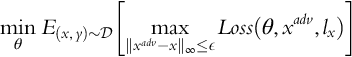
Defense of neural networks against adversarial examples is more difficult compared to generating attacks. Madry et al. (2017) propose a generic saddle point formulation, where ![]() is the underlying training data distribution and Loss(θ, x, lx) is a loss function at data point x with ground-truth label lx for a model with parameter θ:
is the underlying training data distribution and Loss(θ, x, lx) is a loss function at data point x with ground-truth label lx for a model with parameter θ:
This formulation uses robust optimization over the expected loss for worst-case adversarial perturbation for the training data. The internal maximization corresponds to finding adversarial examples and can be approximated using IGSM (Kurakin et al., 2016). This approach falls into a category of defenses that use adversarial training (Shaham, Yamada, & Negahban, 2015). Instead of training with only adversarial examples, using a mixture of normal and adversarial examples in the training set has been found to be more effective (Moosavi-Dezfooli et al., 2016; Szegedy et al., 2013). Another alternative is to augment the learning objective with a regularizer term corresponding to the adversarial inputs (Goodfellow et al., 2014). More recently, logit pairing has been shown to be an effective approximation of adversarial regularization (Kannan, Kurakin, & Goodfellow, 2018).
Another category of defense against adversarial attacks on neural networks are defensive distillation methods (Papernot, McDaniel, Jha, et al., 2016). These methods modify the training process of neural networks to make it difficult to launch gradient-based attacks directly on the network. The key idea is to use distillation training technique (Hinton, Vinyals, & Dean, 2015) and hide the gradient between the presoftmax layer and the softmax outputs. Carlini and Wagner (2016) found methods to break this defense by changing the loss function, calculating gradient directly from presoftmax layer and transferring attack from an easy-to-attack network to a distilled network. More recently, Athalye, Carlini, and Wagner (2018) showed that it is possible to bypass several defenses proposed for the white-box setting (Fig. 2.3).
2.6 Summary and Conclusion
This chapter provided an overview of classical and modern statistical-learning theory, and of how numerical optimization can be used to solve the corresponding mathematical problems with an emphasis on UQ. We discussed how ML and artificial intelligence are the fundamental algorithmic building blocks of IoBT to address the decision-making problem that arises in the underlying control, communication, and networking within the IoBT infrastructure in addition to the inevitable part of almost all military-specific applications developed over IoBT. We studied UQ for ML and artificial intelligence within the context of IoBT, which is critical to provide an accurate measure of error over the output in addition to precise output in military settings. We studied how to quantify and minimize the uncertainty with respect to training an ML algorithm in Section 2.4, which led to a broad discussion on stochastic optimization. Next, we discussed UQ in ML, specifically, how to develop ways for a model to know what it doesn’t know. In other words, we want the model to be especially cautious of data that is different from that on which it was trained. Section 2.5 explored the recent emerging trends on adversarial learning, which is a new application of UQ in ML in IoBT in an offensive and defensive capacity.