
Chapter 9 – Aster Windows Functions
“When you go into court, you are putting your fate into the hands of twelve people who weren’t smart enough to get out of jury duty.”
- Norm Crosby
Cumulative Sum
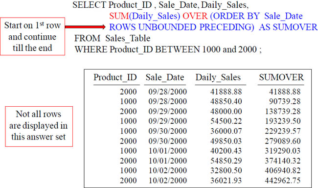
This ANSI version of CSUM is SUM() Over. Right now, the syntax wants to see the sum of the Daily_Sales after it is first sorted by Sale_Date. Rows Unbounded Preceding makes this a CSUM. The ANSI Syntax seems difficult but only at first.
Cumulative Sum - Major and Minor Sort Key(s)
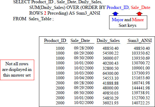
SELECT Product_ID , Sale_Date, Daily_Sales,
SUM(Daily_Sales) OVER (ORDER BY Product_ID, Sale_Date
ROWS UNBOUNDED PRECEDING) AS SumOVER
FROM Sales_Table ;
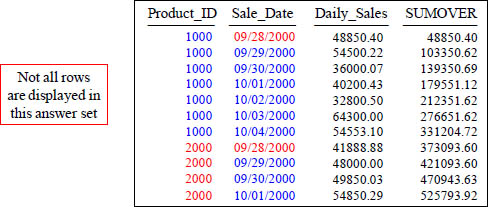
You can have more than one SORT KEY. In the top query, Product_ID is the MAJOR Sort and Sale_Date is the MINOR Sort.
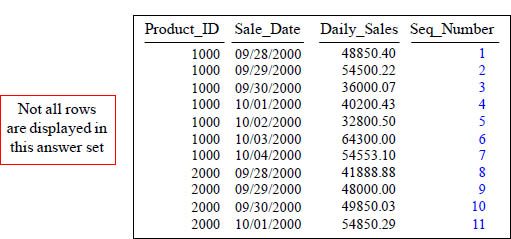
The ANSI CSUM – Getting a Sequential Number
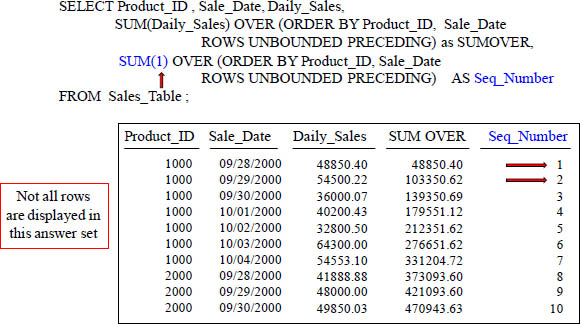
With “Seq_Number”, because you placed the number 1 in the area which calculates the cumulative sum, it’ll continuously add 1 to the answer for each row.
The ANSI OLAP – Reset with a PARTITION BY Statement
SELECT Product_ID , Sale_Date, Daily_Sales,
SUM(Daily_Sales) OVER (PARTITION BY Product_ID
ORDER BY Product_ID, Sale_Date
ROWS UNBOUNDED PRECEDING) AS SumANSI
FROM Sales_Table ;
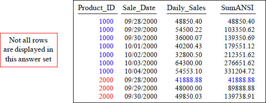
The PARTITION Statement is how you reset in ANSI. This will cause the SUMANSI to start over (reset) on its calculating for each NEW Product_ID.
PARTITION BY only Resets a Single OLAP not ALL of them
SELECT Product_ID , Sale_Date, Daily_Sales,
SUM(Daily_Sales) OVER (PARTITION BY Product_ID
ORDER BY Product_ID, Sale_Date
ROWS UNBOUNDED PRECEDING) AS Subtotal,
SUM(Daily_Sales) OVER (ORDER BY Product_ID, Sale_Date
ROWS UNBOUNDED PRECEDING) AS GRANDTotal
FROM Sales_Table ;
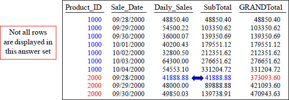
Above are two OLAP statements. Only one has PARTITION BY, so only it resets.
ANSI Moving Sum is Current Row and Preceding n Rows
The SUM () Over allows you to do is to get the moving SUM of a certain column.
How ANSI Moving SUM Handles the Sort
The SUM OVER places the sort after the ORDER BY.
Quiz – How is that Total Calculated?
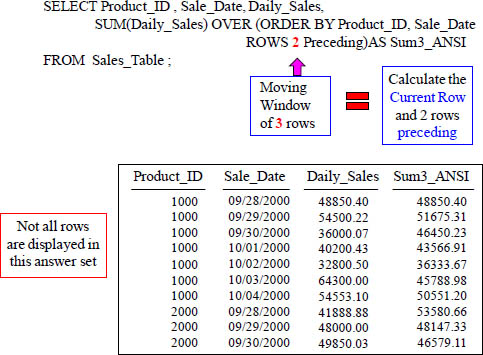
SELECT Product_ID , Sale_Date, Daily_Sales,
SUM(Daily_Sales) OVER (ORDER BY Product_ID, Sale_Date
ROWS 2 Preceding) AS Sum3_ANSI
FROM Sales_Table ;
With a Moving Window of 3, how is the 139350.69 amount derived in the Sum3_ANSI column in the third row?
Answer to Quiz – How is that Total Calculated?
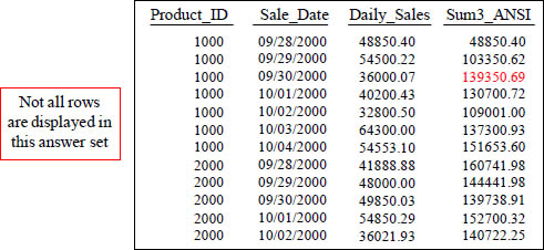
SELECT Product_ID , Sale_Date, Daily_Sales,
SUM(Daily_Sales) OVER (ORDER BY Product_ID, Sale_Date
ROWS 2 Preceding) AS Sum3_ANSI
FROM Sales_Table ;
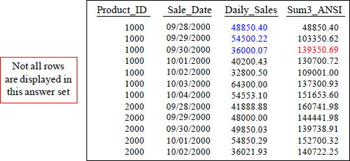
With a Moving Window of 3, how is the 139350.69 amount derived in the Sum3_ANSI column in the third row? It is the sum of 48850.40, 54500.22 and 36000.07. The current row of Daily_Sales plus the previous two rows of Daily_Sales.
Moving SUM every 3-rows vs. a Continuous Sum
SELECT Product_ID , Sale_Date, Daily_Sales,
SUM(Daily_Sales) OVER (ORDER BY Product_ID, Sale_Date
ROWS 2 Preceding) AS SUM3,
SUM(Daily_Sales) OVER (ORDER BY Product_ID, Sale_Date
ROWS UNBOUNDED Preceding) AS Continuous
FROM Sales_Table;
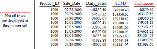
The ROWS 2 Preceding gives the MSUM for every 3 rows. The ROWS UNBOUNDED Preceding gives the continuous MSUM.
Moving Average
Much like the SUM OVER Command, the Average OVER places the sort keys via the ORDER BY keywords.
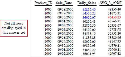
Quiz – How is that Total Calculated?
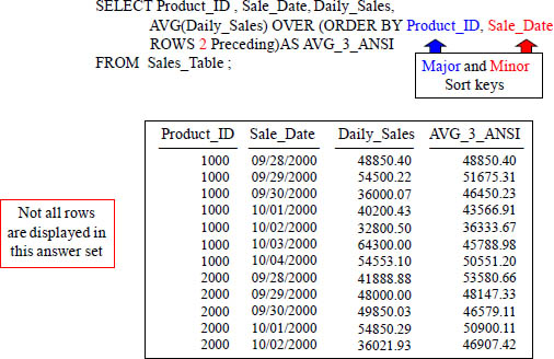
SELECT Product_ID , Sale_Date, Daily_Sales,
AVG(Daily_Sales) OVER (ORDER BY Product_ID, Sale_Date
ROWS 2 Preceding) AS AVG_3_ANSI
FROM Sales_Table ;
With a Moving Window of 3, how is the 46450.23 amount derived in the AVG_3_ANSI column in the third row?
Answer to Quiz – How is that Total Calculated?
SELECT Product_ID , Sale_Date, Daily_Sales,
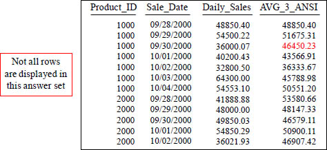
AVG(Daily_Sales) OVER (ORDER BY Product_ID, Sale_Date
ROWS 2 Preceding) AS AVG_3_ANSI
FROM Sales_Table ;
AVG of 48850.40, 54500.22, and 36000.07
Quiz – How is that 4th Row Calculated?
SELECT Product_ID , Sale_Date, Daily_Sales,
AVG(Daily_Sales) OVER (ORDER BY Product_ID, Sale_Date
ROWS 2 Preceding) AS AVG_3_ANSI
FROM Sales_Table ;
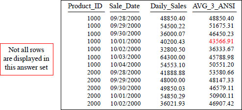
With a Moving Window of 3, how is the 43566.91 amount derived in the AVG_3_ANSI column in the fourth row?
Answer to Quiz – How is that 4th Row Calculated?
SELECT Product_ID , Sale_Date, Daily_Sales,
AVG(Daily_Sales) OVER (ORDER BY Product_ID, Sale_Date
ROWS 2 Preceding) AS AVG_3_ANSI
FROM Sales_Table ;
AVG of 54500.22, 36000.07, and 40200.43
With a Moving Window of 3, how is the 43566.91 amount derived in the AVG_3_ANSI column in the fourth row? The current row plus Rows 2 Preceding.
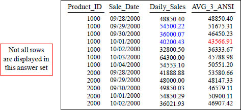
Partition By Resets an ANSI OLAP
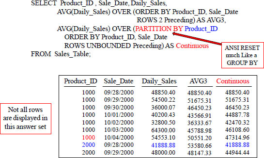
Use a PARTITION BY Statement to Reset the ANSI OLAP. The Partition By statement only resets the column using the statement. Notice that only Continuous resets.
Moving Average Using BETWEEN
SELECT Product_ID , Sale_Date, Daily_Sales,
AVG(Daily_Sales) OVER (ORDER BY Product_ID, Sale_Date
ROWS 2 Preceding)AS AVG_3_ANSI,
AVG(Daily_Sales) OVER (ORDER BY Product_ID, Sale_Date
ROWS BETWEEN 2 Preceding and 2 Following) AS AVG_Between
FROM Sales_Table ;
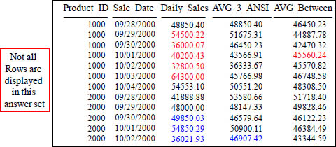
You can also define a ROWS-based frame using constant-offset endpoints relative to the CURRENT ROW. This is displayed above with ROWS BETWEEN 2 PRECEDING AND 2 FOLLOWING. This window frame represents a sliding window of five rows (two preceding, two following, and the current row) and is useful for computing a moving average.
Moving Difference using ANSI Syntax
SELECT Product_ID, Sale_Date, Daily_Sales,
Daily_Sales - SUM(Daily_Sales)
OVER ( ORDER BY Product_ID ASC, Sale_Date ASC
ROWS BETWEEN 4 PRECEDING AND 4 PRECEDING) AS "MDiff_ANSI"
FROM Sales_Table ;
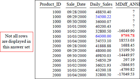
This is how you do an MDiff using the ANSI Syntax with a moving window of 4.
Moving Difference using ANSI Syntax with Partition By
SELECT Product_ID, Sale_Date , Daily_Sales,
Daily_Sales - SUM(Daily_Sales) OVER (PARTITION BY Product_ID
ORDER BY Product_ID ASC, Sale_Date ASC
ROWS BETWEEN 4 PRECEDING AND 4 PRECEDING) AS "MDiff_ANSI"
FROM Sales_Table;
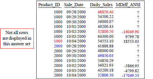
Wow! This is how you do an MDiff using the ANSI Syntax with a moving window of 4 and with a PARTITION BY statement.
RANK Defaults to Ascending Order
SELECT Product_ID ,Sale_Date , Daily_Sales,
RANK() OVER (ORDER BY Daily_Sales) AS Rank1
FROM Sales_Table
WHERE Product_ID IN (1000, 2000) ;
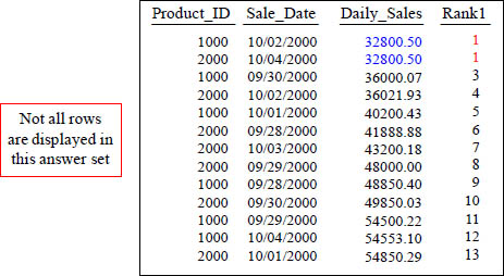
This is the RANK() OVER. It provides a rank for your queries. Notice how you do not place anything within the () after the word RANK. Default Sort is ASC.
Getting RANK to Sort in DESC Order
SELECT Product_ID ,Sale_Date , Daily_Sales,
RANK() OVER (ORDER BY Daily_Sales DESC) AS Rank1
FROM Sales_Table
WHERE Product_ID IN (1000, 2000) ;
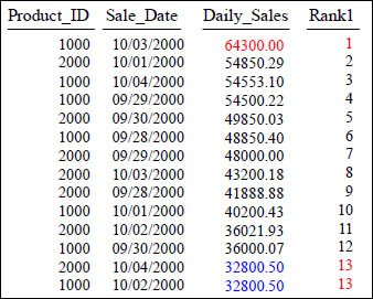
Is the query above in ASC mode or DESC mode for sorting?
You can use Window Functions in Expressions
SELECT Product_ID ,Sale_Date , Daily_Sales,
RANK() OVER (ORDER BY Daily_Sales DESC) -1 AS Rank1
FROM Sales_Table
WHERE Product_ID IN (1000, 2000) ;
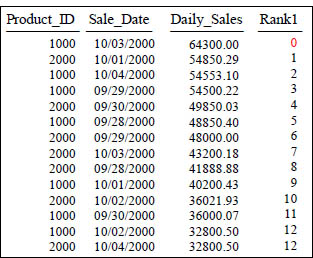
You can use window functions in expressions. Notice the -1 in the query and how it set the first rank to 0.
RANK() OVER and PARTITION BY
SELECT Product_ID ,Sale_Date , Daily_Sales,
RANK() OVER (PARTITION BY Product_ID
ORDER BY Daily_Sales DESC) AS Rank1
FROM Sales_Table
WHERE Product_ID IN (1000, 2000) ;
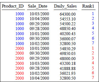
What does the PARTITION Statement in the RANK() OVER do? It resets the rank.
DENSE_RANK() OVER
SELECT Product_ID ,Sale_Date , Daily_Sales,
DENSE_RANK() OVER ( ORDER BY Daily_Sales ) AS DenseRank1
FROM Sales_Table WHERE Product_ID in (1000, 2000) ;
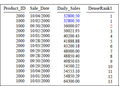
The Dense_Rank command uses the same number for ties, but notice that there is no gap between Rank 1 and Rank 2. Dense_Rank never has a skip or a gap of numbers.
PERCENT_RANK() OVER
SELECT Product_ID ,Sale_Date , Daily_Sales,
PERCENT_RANK() OVER (PARTITION BY PRODUCT_ID
ORDER BY Daily_Sales DESC) AS PercentRank1
FROM Sales_Table WHERE Product_ID in (1000, 2000) ;
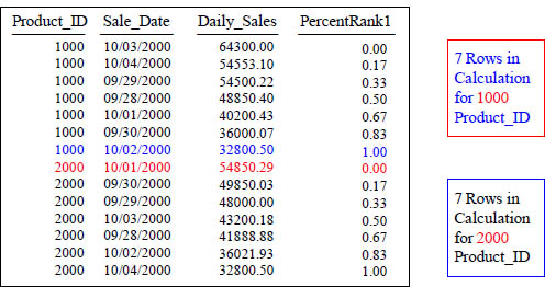
Percent_Rank assigns a relative rank to each row, using the formula: (rank- 1) / (total rows - 1). Now, notice the calculation has a total of 7 rows in two partitions.
PERCENT_RANK() OVER with 14 rows in Calculation
SELECT Product_ID ,Sale_Date , Daily_Sales,
PERCENT_RANK() OVER ( ORDER BY Daily_Sales DESC) AS PercentRank1
FROM Sales_Table WHERE Product_ID IN (1000, 2000) ;
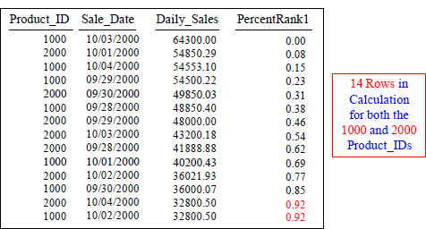
Percent_Rank assigns a relative rank to each row, using the formula: (rank- 1) / (total rows - 1). The ordering of the rows is required. The tie-breaker behavior, when rows are equal in the sort order are sorted arbitrarily within the tie, and the sorted-as-equal rows get the same percent rank number.
PERCENT_RANK() OVER with 21 rows in Calculation
SELECT Product_ID ,Sale_Date , Daily_Sales,
PERCENT_RANK() OVER ( ORDER BY Daily_Sales DESC) AS PercentRank1
FROM Sales_Table ;
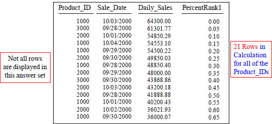
Percent_Rank assigns a relative rank to each row, using the formula: (rank- 1) / (total rows - 1). Now, notice the calculation has changed because we are calculating 21 rows.
RANK With ORDER BY SUM()
SELECT Product_ID , SUM(Daily_Sales),
RANK() OVER
(ORDER BY SUM(Daily_Sales) DESC ) AS Product_Sales_Rank
FROM Sales_Table
GROUP BY Product_ID ;
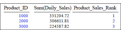
You can also use SQL aggregates inside the OVER clause, as shown in the ORDER BY clause above. In this example, the PARTITION BY clause has been omitted. This causes the window function to compute the window function over all the data. This could have significant impact because all data must be processed at one node.
COUNT OVER for a Sequential Number
SELECT Product_ID ,Sale_Date , Daily_Sales,
COUNT(*) OVER (ORDER BY Product_ID, Sale_Date
ROWS UNBOUNDED PRECEDING) AS Seq_Number
FROM Sales_Table WHERE Product_ID IN (1000, 2000) ;
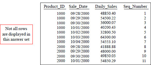
This is the COUNT OVER. It will provide a sequential number starting at 1. The Keyword(s) ROWS UNBOUNDED PRECEDING causes Seq_Number to start at the beginning and increase sequentially to the end.
Quiz – What caused the COUNT OVER to Reset?
SELECT Product_ID ,Sale_Date , Daily_Sales,
COUNT(*) OVER (PARTITION BY Product_ID
ORDER BY Product_ID, Sale_Date
ROWS UNBOUNDED PRECEDING) AS StartOver
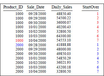
FROM Sales_Table WHERE Product_ID IN (1000, 2000) ;
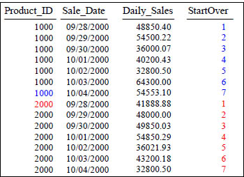
What Keyword(s) caused StartOver to reset?
Answer to Quiz – What caused the COUNT OVER to Reset?
SELECT Product_ID ,Sale_Date , Daily_Sales,
COUNT(*) OVER (PARTITION BY Product_ID
ORDER BY Product_ID, Sale_Date
ROWS UNBOUNDED PRECEDING) AS StartOver
FROM Sales_Table WHERE Product_ID IN (1000, 2000) ;
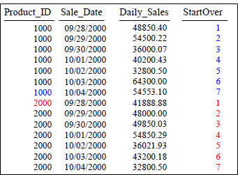
What Keyword(s) caused StartOver to reset? It is the PARTITION BY statement.
The MAX OVER Command
SELECT Product_ID ,Sale_Date , Daily_Sales,
MAX(Daily_Sales) OVER (ORDER BY Product_ID, Sale_Date
ROWS UNBOUNDED PRECEDING) AS MaxOver
FROM Sales_Table WHERE Product_ID IN (1000, 2000) ;
After the sort the Max() Over shows the Max Value up to that point.
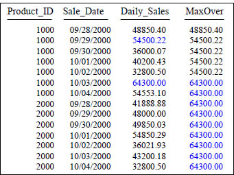
MAX OVER with PARTITION BY Reset
SELECT Product_ID ,Sale_Date , Daily_Sales,
MAX(Daily_Sales) OVER (PARTITION BY Product_ID
ORDER BY Product_ID, Sale_Date
ROWS UNBOUNDED PRECEDING) AS MaxOver
FROM Sales_Table WHERE Product_ID IN (1000, 2000) ;
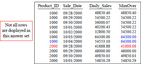
The largest value is 64300.00 in the column MaxOver. Once it was evaluated, it did not continue until the end because of the PARTITION BY reset.
The MIN OVER Command
SELECT Product_ID, Sale_Date ,Daily_Sales
,MIN(Daily_Sales) OVER (ORDER BY Product_ID, Sale_Date
ROWS UNBOUNDED PRECEDING) AS MinOver
FROM Sales_Table WHERE Product_ID IN (1000, 2000) ;
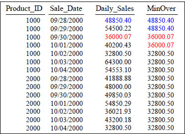
After the sort, the MIN () Over shows the Max Value up to that point.
Quiz – Fill in the Blank
SELECT Product_ID ,Sale_Date , Daily_Sales,
MIN(Daily_Sales) OVER (PARTITION BY Product_ID
ORDER BY Product_ID, Sale_Date
ROWS UNBOUNDED PRECEDING) AS MinOver
FROM Sales_Table WHERE Product_ID IN (1000, 2000) ;
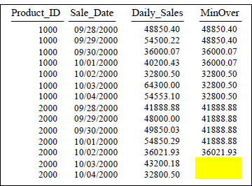
The last two answers (MinOver) are blank, so you can fill in the blank.
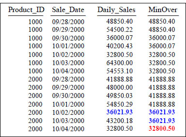
Answer to Quiz – Fill in the Blank
SELECT Product_ID ,Sale_Date , Daily_Sales,
MIN(Daily_Sales) OVER (PARTITION BY Product_ID
ORDER BY Product_ID, Sale_Date
ROWS UNBOUNDED PRECEDING) AS MinOver
FROM Sales_Table WHERE Product_ID IN (1000, 2000) ;
The Row_Number Command
SELECT Product_ID ,Sale_Date , Daily_Sales,
ROW_NUMBER() OVER (ORDER BY Product_ID, Sale_Date) AS Seq_Number
FROM Sales_Table WHERE Product_ID IN (1000, 2000) ;
The ROW_NUMBER() Keyword(s) caused Seq_Number to increase sequentially. Notice that this does NOT have a Rows Unbounded Preceding and it still works!
Quiz – How did the Row_Number Reset?
SELECT Product_ID ,Sale_Date , Daily_Sales,
ROW_NUMBER() OVER (PARTITION BY Product_ID
ORDER BY Product_ID, Sale_Date ) AS StartOver
FROM Sales_Table WHERE Product_ID IN (1000, 2000) ;
What Keyword(s) caused StartOver to reset?
Quiz – How did the Row_Number Reset?
SELECT Product_ID ,Sale_Date , Daily_Sales,
ROW_NUMBER() OVER (PARTITION BY Product_ID
ORDER BY Product_ID, Sale_Date ) AS StartOver
FROM Sales_Table WHERE Product_ID IN (1000, 2000) ;
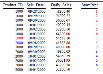
What Keyword(s) caused StartOver to reset? It is the PARTITION BY statement.
NTILE
SELECT Product_ID ,Sale_Date , Daily_Sales,
NTILE(4) OVER (ORDER BY Daily_Sales) AS Bucket
FROM Sales_Table WHERE Product_ID IN (1000, 2000) ;
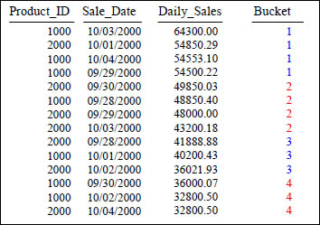
The NTILE() function divides the rows into buckets as evenly as possible. In this example, because PARTITION BY is omitted, the entire input will be sorted using the ORDER BY clause and then divided into the number of buckets specified.
NTILE Using a Value of 10
SELECT Product_ID ,Sale_Date , Daily_Sales,
NTILE(10) OVER (ORDER BY Daily_Sales) AS Bucket
FROM Sales_Table WHERE Product_ID IN (1000, 2000) ;
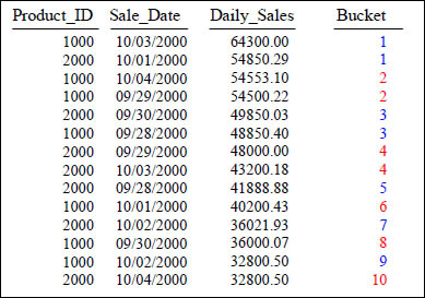
The NTILE() function divides the rows into buckets as evenly as possible. In this example, because PARTITION BY is omitted, the entire input will be sorted using the ORDER BY clause and then divided into the number of buckets specified. This example uses a value of 10 in the NTILE.
NTILE With a Partition
SELECT Product_ID ,Sale_Date , Daily_Sales,
NTILE(3) OVER (PARTITION BY Product_ID
ORDER BY Daily_Sales) AS Bucket
FROM Sales_Table WHERE Product_ID IN (1000, 2000) ;
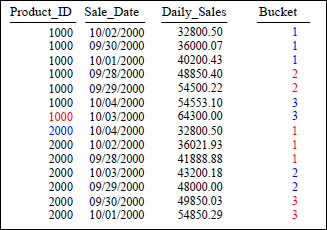
The NTILE() function divides the rows into buckets as evenly as possible. In this example, because PARTITION BY is listed, the data will first be sorted by Product_ID and then sorted using the ORDER BY clause (within Product_ID) and then divided into the number of buckets specified. This example uses a value of 3 in the NTILE. Notice that the PARTITION BY statement causes the answer set to reset when the Product_ID goes from 1000 to 2000.
CUME_DIST
SELECT Product_ID ,Sale_Date , Daily_Sales,
CUME_DIST() OVER (ORDER BY Daily_Sales DESC) AS CDist
FROM Sales_Table WHERE Product_ID IN (1000, 2000) ;
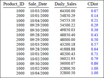
The CUME_DIST() is a cumulative distribution function that assigns a relative rank to each row based on a formula. That formula is: (number of rows preceding or peer with current row) / (total rows). We order by Daily_Sales DESC so that each row is ranked by cumulative distribution. The distribution is represented relatively by floating point numbers from 0 to 1. When there is only one row in a partition, it is assigned 1. When there are more than one row, they are assigned a cumulative distribution ranking ranging from 0 to 1.
CUME_DIST With a Partition
SELECT Product_ID ,Sale_Date , Daily_Sales,
CUME_DIST() OVER (PARTITION by Product_ID
ORDER BY Daily_Sales DESC) AS CDist
FROM Sales_Table WHERE Product_ID IN (1000, 2000) ;
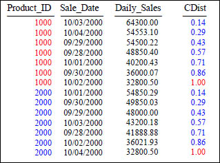
The CUME_DIST() is a cumulative distribution function that assigns a relative rank to each row based on a formula. That formula is: (number of rows preceding or peer with current row) / (total rows). We Partition by Product_ID and then Order By Daily_Sales DESC so that each row is ranked by cumulative distribution within its partition.
LEAD
SELECT Product_ID ,Sale_Date , Daily_Sales,
Daily_Sales - LEAD(Daily_Sales, 1, 0)
OVER (ORDER BY Product_ID, Sale_Date) AS Lead1
FROM Sales_Table WHERE Product_ID IN (1000, 2000) ;
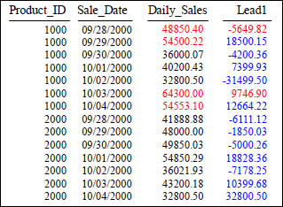
Above, we compute the difference between a product's Daily_Sales and that of the next Daily_Sales in the sort order (which will be the next row's Daily_Sales, or one whose Daily_Sales is the same). The expression LEAD(Daily_Sales, 1, 0) tells LEAD() to evaluate the expression Daily_Sales on the row that is positioned one row following the current row. If there is no such row (as is the case on the last row of the partition or relation), then the default value of 0 is used.
LEAD With Partitioning
SELECT Product_ID ,Sale_Date , Daily_Sales,
Daily_Sales - LEAD(Daily_Sales, 1, 0)
OVER (PARTITION BY Product_ID ORDER BY Sale_Date) AS Lead1
FROM Sales_Table WHERE Product_ID IN (1000, 2000) ;
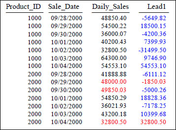
Above, we compute the difference between a product's Daily_Sales and that of the next Daily_Sales in the sort order (which will be the next row's Daily_Sales, or one whose Daily_Sales is the same). We also partitioned the data by Product_ID.
LAG
SELECT Product_ID ,Sale_Date , Daily_Sales,
Daily_Sales - LAG(Daily_Sales, 1, 0)
OVER (ORDER BY Product_ID, Sale_Date) AS Lag1
FROM Sales_Table WHERE Product_ID IN (1000, 2000) ;
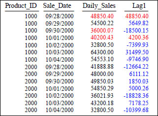
Above, we compute the difference between a product's Daily_Sales and that of the next Daily_Sales in the sort order (which will be the previous row's Daily_Sales, or one whose Daily_Sales is the same). The expression LAG(Daily_Sales, 1, 0) tells LAG() to evaluate the expression Daily_Sales on the row that is positioned one row before the current row. If there is no such row (as is the case on the first row of the partition or relation), then the default value of 0 is used.
LAG with Partitioning
SELECT Product_ID ,Sale_Date , Daily_Sales,
Daily_Sales - LAG(Daily_Sales, 1, 0)
OVER (PARTITION BY Product_ID ORDER BY Sale_Date) AS Lag1
FROM Sales_Table WHERE Product_ID IN (1000, 2000) ;
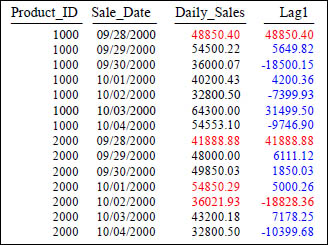
Above, we compute the difference between a product's Daily_Sales and that of the next Daily_Sales in the sort order (which will be the previous row's Daily_Sales, or one whose Daily_Sales is the same). The expression LAG(Daily_Sales, 1, 0) tells LAG() to evaluate the expression Daily_Sales on the row that is positioned one row before the current row. If there is no such row (as is the case on the first row of the partition or relation), then the default value of 0 is used.
FIRST_VALUE
SELECT Product_ID ,Sale_Date , Daily_Sales,
Daily_Sales - First_Value (Daily_Sales)
OVER (ORDER BY Sale_Date) AS Delta_First
FROM Sales_Table WHERE Product_ID IN (1000, 2000) ;
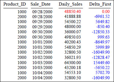
Above, after sorting the data by Sale_Date, we compute the difference between the first row's Daily_Sales and the Daily_Sales of each following row. All rows Daily_Sales are compared with the first row's Daily_Sales, thus the name First_Value.
FIRST_VALUE After Sorting by the Highest Value
SELECT Product_ID ,Sale_Date , Daily_Sales,
Daily_Sales - First_Value (Daily_Sales)
OVER (ORDER BY Daily_Sales DESC) AS Delta_First
FROM Sales_Table WHERE Product_ID IN (1000, 2000) ;
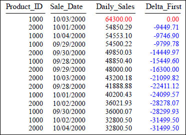
Above, after sorting the data by Daily_Sales DESC, we compute the difference between the first row's Daily_Sales and the Daily_Sales of each following row. All rows Daily_Sales are compared with the first row's Daily_Sales, thus the name First_Value. This example shows how much less each Daily_Sales is compared to 64,300.00 (our highest sale).
FIRST_VALUE with Partitioning
SELECT Product_ID ,Sale_Date , Daily_Sales,
Daily_Sales - First_Value (Daily_Sales)
OVER (PARTITION BY Product_ID
ORDER BY Sale_Date) AS Delta_First
FROM Sales_Table WHERE Product_ID IN (1000, 2000) ;
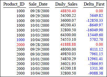
We are now comparing the Daily_Sales of the first Sale_Date for each Product_ID with the Daily_Sales of all other rows within the Product_ID partition. Each row is only compared with the first row (First_Value) in its partition.
LAST_VALUE
SELECT Product_ID ,Sale_Date , Daily_Sales,
Daily_Sales - LAST_Value (Daily_Sales)
OVER (ORDER BY Sale_Date) AS Delta_Last
FROM Sales_Table WHERE Product_ID IN (1000, 2000) ;
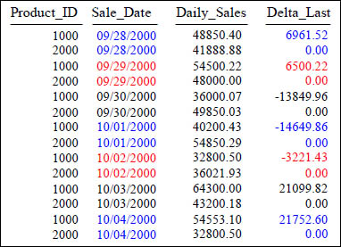
Above, after sorting the data by Sale_Date, we compute the difference between the last row's Daily_Sales and the Daily_Sales of each following row (from the same Sale_Date). Since there is only two product totals for each day, there is always a 0.00 for one of the rows.
NTH_VALUE
SELECT Product_ID ,Sale_Date , Daily_Sales,
NTH_Value (Daily_Sales, 2)
OVER (ORDER BY Sale_Date) AS Nth_Val
FROM Sales_Table WHERE Product_ID IN (1000, 2000) ;
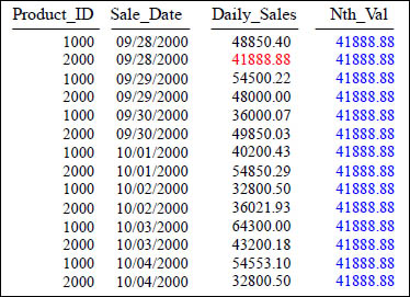
Above, after sorting the data by Sale_Date, we list the value of the second row for Daily_Sales. The second row in the answer set had a value of 41,888.88 for its Daily_Sales. That value is placed in each row for Nth_Val.
NTH_VALUE With Partition
SELECT Product_ID ,Sale_Date , Daily_Sales,
NTH_Value (Daily_Sales, 3) OVER (PARTITION BY Product_ID
ORDER BY Sale_Date) AS Nth_Val
FROM Sales_Table WHERE Product_ID IN (1000, 2000) ;
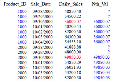
Above, after Partition the data by Product_ID and then sorting the data by Sale_Date, we list the value of the third row for Daily_Sales (per partition). Notice that rows one and two in each Partition have Null values.
SUM(SUM(n))
SELECT Product_ID , SUM(Daily_Sales),
SUM(SUM(Daily_Sales)) OVER (ORDER BY Sum(Daily_Sales) )
AS Prod_Sales_Running_Sum
FROM Sales_Table
GROUP BY Product_ID ;
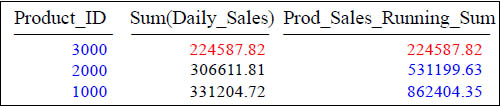
Window functions can compute aggregates of aggregates as in the example above.