Search in book...
Toggle Font Controls
Create new playlist

Name your new playlist

Playlist description (optional)
Sign In

Email address

Password

Forgot Password?

or

Continue with Facebook

Continue with Google
Sign Up

Full Name

Email address

Confirm Email Address

Password

or

Continue with Facebook

Continue with Google

Previous Chapter

Back Matter

M. Ottina et al.Automated Market Makershttps://doi.org/10.1007/978-1-4842-8616-6_5

5. Uniswap v3

Miguel Ottina¹, Peter Johannes Steffensen² and Jesper Kristensen³

(1)

Rivadavia, Argentina

(2)

Aarhus, Denmark

(3)

New York, NY, USA

Uniswap v3 turns out to be very different from Uniswap v2. Although Uniswap v3 pools also have two tokens and use a constant product formula, Uniswap v3 introduces a new concept that is called concentrated liquidity. The main idea of this feature is that liquidity providers can provide liquidity in a chosen price range and implies that the reserves of each position are just enough to support trading within its range. When the price goes out of that range, the position of the liquidity provider is swapped entirely into one of the two tokens, depending on the price going above or below the range.

A consequence of concentrated liquidity is that the positions are highly personalized, since liquidity providers can choose not only the amount to deposit but also the range in which they want to provide liquidity. This implies that the positions in a Uniswap v3 pool are naturally nonfungible. Therefore, liquidity providers must be given nonfungible tokens in exchange for their deposit, and these nonfungible LP tokens will have to keep a record of the details of their particular position. In addition, due to the customizable liquidity provision feature, fees must now be collected and stored separately as individual tokens rather than being automatically reinvested as liquidity into the pool.

In this chapter, we will present a thorough exposition of the Uniswap v3 AMM, together with a comprehensive analysis of liquidity provisioning in this protocol. We will also explain in detail how this AMM is actually implemented.

5.1 Ticks

As we mentioned before, in Uniswap v3, liquidity providers provide liquidity in a chosen bounded price range. However, the lower and upper limits of this range cannot be defined arbitrarily but rather can be chosen from a finite (but very big!) subset of the set of real positive numbers. The elements of this subset are called ticks and are indexed by integer numbers in the following way: i ∈ ℤ represents the tick (and hence the price) p(i) = 1.0001ⁱ. We will also say that the tick index for the tick p(i) is i.

Note that each tick is 0.01% away from the following tick. Uniswap v3 uses 24-bit signed integers for tick indexes. Hence, the minimum and maximum prices that it can deal with are

$pleft(-{2}^{23} ight)approx 5.07cdot {10}^{-365}$

and

$pleft({2}^{23}-1 ight)approx 1.97cdot {10}^{364}$

which cover almost all possible prices in the asset space.

As we mentioned before, Uniswap v3 is based on the constant product formula of Uniswap v2. Recall that in a Uniswap v2 pool, the balances A and B of the two tokens, X and Y, of the pool satisfy the formula A ⋅ B = L², where L is the liquidity parameter of the pool. Recall also that the spot price p of token X in terms of token Y is given by $frac{B}{A}$ . Hence, we can express the balances A and B in terms of L and $$ sqrt{p} $$

in the following way:

$A=frac{L}{sqrt{p}}kern1em extrm{and}kern1em B=Lcdot sqrt{p}.$

Therefore, L and $$ sqrt{p} $$

can be used to track the state of the pool, and this is what the Uniswap v3 AMM does. Note that

$sqrt{p}(i)={1.0001}^{frac{i}{2}}$

Given any price p, the tick index associated to p is defined as the tick index of the greatest tick t that satisfies t ≤ p. Hence, the tick index i associated to the price p is given by

$i=leftlfloor {log}_{1.0001};p ight floor =leftlfloor 2{log}_{1.0001}sqrt{p} ight floor,$

(5.1)

where for any real number x, ⌊x⌋ denotes the floor of x, that is, the greatest integer that is less than or equal to x.

Example 5.1. Consider a Uniswap v3 pool with tokens ETH and DAI with the following balances:

Tokens	DAI	ETH
Balances	40,000	10

Note that the current spot price is 4,000 DAI/ETH. This price is associated, via Equation 5.1, to the tick index

$i=leftlfloor {log}_{1.0001}4000 ight floor =82944.$

Observe that the tick index 82,944 corresponds to the price

${1.0001}^{82944}approx 3999.742678$

while the tick index 82,945 corresponds to the price

${1.0001}^{82945}approx 4000.142653.$

If a liquidity provider wants to provide liquidity in the price range [3700, 4300], then we can find the tick indexes that are near the limits of this interval by applying Equation 5.1:

$leftlfloor {log}_{1.0001}3700 ight floor =82164,leftlfloor {log}_{1.0001}4300 ight floor =83667.$

Now, we compute the ticks that correspond to these tick indexes and to the following ones, since the prices that we are interested in will be between those ticks. We exhibit the computations in the following table:

Tick index	82,164	82,165	83,667	83,668
Tick (approx.)	3,699.634	3,700.004	4,299.619	4,300.049

Hence, the liquidity provider can choose to provide liquidity in the price interval [3,700.004, 4,300.049].

5.1.1 Initialized Ticks

In Uniswap v3, ticks can have one of the following two states: initialized or uninitialized. The initialized ticks are those ticks that define the boundary of any of the current positions (see Figure 5-1). In other words, the initialized ticks are those ticks that we need to take care of, because the liquidity parameter can change when the price crosses the tick since a different set of positions needs to be considered. By introducing initialized ticks, the Uniswap v3 protocol avoids having to make computations and update variable values every time the price crosses a tick, since this is needed only when the price crosses an initialized tick.

If a tick is used in a new position and that tick has not been initialized yet, then the tick is initialized. If a tick is a boundary of only one position, when that position is removed, the tick is uninitialized. In order to keep track of initialized and uninitialized ticks, Uniswap v3 introduces a tick bitmap, where each bitmap position corresponds to a tick index. If the tick is initialized, the value of the bitmap position that corresponds to that tick is 1, and if the tick is uninitialized, the value of the bitmap position that corresponds to that tick is 0.

5.1.2 Tick Spacing

In Example 5.1, we did not impose any restrictions on the tick indexes, and hence, any 24-bit signed integer could be a tick index. In general, Uniswap v3 does not allow an arbitrary choice of the tick indexes but rather introduces the concept of tick spacing, which, in informal terms, is a measure of the separation between the allowed tick indexes. Concretely, only tick indexes that are multiples of the tick spacing are permitted. For example, if the tick spacing is 5, the only tick indexes that can be used are the multiples of 5: …, –10, –5, 0, 5, 10,….

In the previous example, if the tick spacing had been equal to 5, we would have had to consider the following table and the liquidity provider could have chotsen to provide liquidity in the price interval [3700.004, 4300.909].

Tick index	82,160	82,165	83,665	83,670
Tick (approx.)	3,698.155	3,700.004	4,298.759	4,300.909

The tick spacing parameter is defined and fixed when the pool is created. Clearly, if the tick spacing is small, then liquidity providers can choose more precise ranges, but on the other hand, a small tick spacing may cause trading to be more expensive in terms of gas fees, since every time the price crosses an initialized tick, new values for certain variables need to be set, which imposes a gas cost on the trader.

5.2 Liquidity Providers’ Position

Consider a Uniswap v3 liquidity pool with tokens X and Y. From now on, when we speak about the price, we will be referring to the price of token X in terms of token Y. Suppose that a liquidity provider provides liquidity in a price range [p_a, p_b]. The main idea of Uniswap v3 is that the liquidity provider’s position will use its assets to allow trading between the prices p_a and p_b. When the price goes out of this range, the position’s assets are not used for trading, and hence, the position’s balances remain unmodified until the price enters the interval [p_a, p_b] again. In addition, if the price falls below p_a, then the liquidity provider’s position will be fully converted to token X, and if the price goes above p_b, then the liquidity provider’s position will be fully converted to token Y. For example, in this last case, we can think that the whole amount of token X of the position has been sold as the price of token X increased, and thus, the position only has token Y left. Note that in both cases, the liquidity provider is left with the asset that is less valuable.

Although the Uniswap v3 AMM is based on the constant product formula, some modifications need to take place in order to allow the balance of one of the tokens to become zero when the price reaches one of the boundaries of the interval. Concretely, we will apply the translation shown in Figure 5-2 to the curve defined by the constant product formula xy = L². Recall from subsection 2.1.1 that in this case, the price at a state P coincides with the slope of the line that passes through the points (0, 0) and P, and hence, in Figure 5-2, the price p_a at the pool state a is less than the price p_b at the pool state b.

Figure 5-2
Translation applied to the constant product formula in Uniswap v3

In order to find the parameters of the translation that we need to apply, we will compute the balances of the tokens at the pool states a and b. Let x_a and y_a be the balances at state a of tokens X and Y, respectively. Clearly, x_ay_a = L², and since the spot price at state a is p_a, we obtain that $frac{y_a}{x_a}={p}_a$ Hence, ${x}_a=frac{L}{sqrt{p_a}}$ and ${y}_a=Lsqrt{p_a}$ Thus, $a=left(frac{L}{sqrt{p_a}},Lsqrt{p_a} ight)$ . In a similar way, we obtain that $b=left(frac{L}{sqrt{p_b}},Lsqrt{p_b} ight)$ .

When the price is p_a, we need that the balance of token Y is equal to zero, or equivalently, that the corresponding state is on the horizontal axis. Thus, we need to make a downward translation of an amount y_a. Similarly, when the price is p_b, we need that the balance of token X is equal to zero, or equivalently, that the corresponding state is on the vertical axis. Thus, we need to make a translation to the left of an amount x_b. Therefore, we will make a translation of the curve defined by xy = L²−which is called curve of virtual balances—by the vector (−x_b, −y_a), that is, $left(-frac{L}{sqrt{p_b}},-Lsqrt{p_a} ight)$ . Hence, we obtain the following equation:

$left(x+frac{L}{sqrt{p_b}} ight)left(y+Lsqrt{p_a} ight)={L}^2$

(5.2)

which defines the curve of real balances given in Figure 5-2.

Observe also that applying the translation mentioned previously to the points a and b, we obtain the points c and d of Figure 5-2, and hence,

$c=left(frac{L}{sqrt{p_a}}-frac{L}{sqrt{p_b}},0 ight)kern1em extrm{and}kern1em d=left(0,Lsqrt{p_b}-Lsqrt{p_a} ight).$

Virtual reserves. We will now introduce the concept of virtual reserves, which will be needed later. With the previous notations, the virtual reserves (or virtual balances) of tokens X and Y are the positive real numbers x_v and y_v that satisfy the constant product formula x_vy_v = L² and the spot price formula $frac{y_v}{x_v}=p$ where p is the spot price of the pool at a certain moment. This means that the virtual reserves define a virtual pool state (x_v, y_v) that is located on the curve of virtual balances of Figure 5-2. We can think that whenever the price belongs to the range [p_a, p_b], the trades in the pool are carried out following the constant product formula x_vy_v = L², although the real reserves of the pool—the actual balances of the tokens—do not coincide with the virtual reserves.

It is important to observe that the real and virtual reserves of a liquidity provider’s position (x and y, and x_v and y_v, respectively) are related by the following equations:

${displaystyle egin{array}{ll}& {x}_v=x+frac{L}{sqrt{p_b}},\ {}& {y}_v=y+Lsqrt{p_a},end{array}}$

(5.3)

and thus, the equations

$left(x+frac{L}{sqrt{p_b}} ight)left(y+Lsqrt{p_a} ight)={L}^2$

and

${x}_v{y}_v={L}^2$

are equivalent.

Note also that if the spot price at a certain moment is p, since $frac{y_v}{x_v}=p$ , we obtain that

${x}_v=frac{L}{sqrt{p}}kern1em extrm{and}kern1em {y}_v=Lsqrt{p}.$

(5.4)

Real reserves at price p. It is important to be able to compute the balances of a liquidity provider’s position when the price is p. Following the previous notations, we know that when p ∈ [p_a, p_b], the balances x and y of the liquidity provider’s position satisfy Equation 5.2, that is,

$left(x+frac{L}{sqrt{p_b}} ight)left(y+Lsqrt{p_a} ight)={L}^2.$

If p = p_a, the balance y of token Y is equal to zero, and hence, isolating x from the previous equation, we obtain that the balance of token X is $frac{L}{sqrt{p_a}}-frac{L}{sqrt{p_b}}$ . Thus, the state of the liquidity provider’s position when p = p_a is $left(frac{L}{sqrt{p_a}}-frac{L}{sqrt{p_b}},0 ight)$ , which are the coordinates of the point c of thecurve of real balances of Figure 5-2 that lies on the horizontal axis. These coordinates could also have been obtained by translating the point a by the vector (−x_b, −y_a), which was the vector used for translating the curve of virtual balances of Figure 5-2 to the curve of real balances.

In a similar way, if p = p_b, the balance x of token X is equal to zero, and isolating y from the previous equation, we obtain that the balance of token Y is $Lsqrt{p_b}-Lsqrt{p_a}$ . In addition, using Figure 5-2, a geometrical interpretation (similar to the previous one) can be made.

In general, for any p ∈ [p_a, p_b], we know from Equation 5.4 that the virtual reserves are

${x}_v=frac{L}{sqrt{p}}kern1em extrm{and}kern1em {y}_v=Lsqrt{p}.$

Thus, applying Equation 5.3, we obtain that

$x=frac{L}{sqrt{p}}-frac{L}{sqrt{p_b}}kern1em extrm{and}kern1em y=Lsqrt{p}-Lsqrt{p_a}.$

Note that in the particular cases p = p_a and p = p_b, we obtain the results of the previous paragraphs again.

Finally, recall that when p < p_a, the balances of the liquidity provider’s position are the same as when p = p_a, since these balances are not used for trades when the price goes outside the interval [p_a, p_b]. Similarly, when p > p_b, the balances of the liquidity provider’s position are the same as when p = p_b. We condense the previous formulae into Table 5-1.

Table 5-1

Formulae for the real balances of a Uniswap v3 position

Price range	Real balance of token X	Real balance of token Y
p ≤ p_a	$frac{L}{sqrt{p_a}}-frac{L}{sqrt{p_b}}$	0
p_a ≤ p ≤ p_b	$frac{L}{sqrt{p}}-frac{L}{sqrt{p_b}}$	$Lsqrt{p}-Lsqrt{p_a}$
p ≥ p_b	0	$Lsqrt{p_b}-Lsqrt{p_a}$

Opening a position. Suppose that a liquidity provider wants to provide liquidity in the price range [p_a, p_b]. Using the notations of this section, if the parameter L is chosen, then the curve of virtual balances of Figure 5-2 is fixed, and thus, the curve of real balances is uniquely determined. Hence, by the previous results, given a price p, the real balances of the liquidity provider’s position are determined. It is important to observe that since the trading fees of Uniswap v3 are stored separately, the parameter L will remain constant, the curves of Figure 5-2 will not change, and the state of the position will always be a point of the curve of real balances.

In consequence, if the liquidity provider wants to start a position with those characteristics−p_a, p_b and L chosen—given the price p, they need to deposit the amounts of tokens X and Y given by Table 5-1 so that the state of their position belongs to the curve of real balances. Concretely, we need to consider the following three possible situations:

(A) If the current price p is below the price range [p_a, p_b] — that is, if p < p_a — the liquidity provider will have to deposit only token X, and the amount of token X they need to deposit is $frac{L}{sqrt{p_a}}-frac{L}{sqrt{p_b}}$ .

(B) If the current price p is within the price range [p_a, p_b]−that is, if p_a ≤ p ≤ p_b−the liquidity provider will need to deposit certain amounts of both tokens. Specifically, they will need to deposit an amount $frac{L}{sqrt{p}}-frac{L}{sqrt{p_b}}$ of token X and an amount $Lsqrt{p}-Lsqrt{p_a}$ of token Y.

(C) If the current price p is above the price range [p_a, p_b]—that is, if p > p_b—the liquidity provider will have to deposit only token Y, and the amount of token Y they need to deposit is $Lsqrt{p_b}-Lsqrt{p_a}$

In Figure 5-3, we can see the corresponding states of the position in the three cases discussed previously.

Figure 5-3
Creating a position in Uniswap v3

Of course, in practice, a liquidity provider will not want to choose the parameter L, but instead, they will choose a price range [p_a, p_b] and a certain amount of either token X or token Y to deposit. In that case, we can simply use that amount and the formulae of Table 5-1 to find out the value of the parameter L, and then use this value to compute the amount of the other token that the liquidity provider needs to deposit. We show how this works in the following example.

Example 5.2. Suppose that a liquidity provider wants to provide liquidity in a Uniswap v3 pool with tokens ETH and USDC. Suppose, in addition, that the price of ETH in terms of USDC is 4,000 and that the liquidity provider wants to deposit liquidity in the price range (3,700.004, 4,300.049) as in Example 5.1, and that the liquidity provider wants to deposit 2 ETH.

In order to find out how much USDC the liquidity provider needs to deposit, we will first compute the value of the parameter L using the formulae of the previous table. Concretely,

$2=frac{L}{sqrt{p}}-frac{L}{sqrt{p_b}}approx frac{L}{sqrt{4000}}-frac{L}{sqrt{4300.049}}=Lleft(frac{1}{sqrt{4000}}-frac{1}{sqrt{4300.049}} ight)$

Hence,

$Lapprox frac{2}{frac{1}{sqrt{4000}}-frac{1}{sqrt{4300.049}}}approx 3561.138.$

Now we use the value of L to compute the amount of USDC that is needed.

$y=Lsqrt{p}-Lsqrt{p_a}approx 3561.138left(sqrt{4000}-sqrt{3700.004} ight)approx 8610.458.$

Therefore, the liquidity provider will have to make a deposit of 2 ETH and 8,610.458 USDC to set up their position.

Value of a position. We will now compute the value of a liquidity provider’s position in terms of the price p, which will be denoted by V(p). If x_p and y_p denote the real reserves of the liquidity provider’s position when the price is p, then V(p) = x_pp + y_p. Note that when the position is set up, the value of the liquidity parameter L and the price range [p_a, p_b] in which liquidity will be provided are fixed. Using the results of Table 5-1, we obtain the following:

If p ≤ p_a, then

$V(p)=left(frac{L}{sqrt{p_a}}-frac{L}{sqrt{p_b}} ight)p=Lleft(frac{1}{sqrt{p_a}}-frac{1}{sqrt{p_b}} ight)p.$

If p_a ≤ p ≤ p_b, then

$V(p)=left(frac{L}{sqrt{p}}-frac{L}{sqrt{p_b}} ight)p+Lsqrt{p}-Lsqrt{p_a}=Lleft(2sqrt{p}-frac{p}{sqrt{p_b}}-sqrt{p_a} ight).$

If p ≥ p_b, then

$V(p)=Lsqrt{p_b}-Lsqrt{p_a}=Lleft(sqrt{p_b}-sqrt{p_a} ight).$

We use the previous formulae to plot, in Figure 5-4, the value of a Uniswap v3 liquidity provider’s position as a function of the price p.

Figure 5-4
Value of a liquidity provider’s position as a function of the price p

Example 5.3. Consider the liquidity provider’s position of Example 5.2, with liquidity parameter L ≈ 3,561.138 and price range (3700.004, 4300.049). The liquidity provider deposited 2 ETH and approximately 8,610.458 USDC when the price of ETH in terms of USDC was 4,000, so the initial value of their position is

$$ V(4000)=2cdot 4000+8610.458=16,610.458; extrm{USDC}. $$

If the price goes up to 4,200, from the formulae of Table 5-1, we obtain that the real balance of ETH in the liquidity provider’s position will be approximately

$frac{3561.138}{sqrt{4200}}-frac{3561.138}{sqrt{4300.049}}approx 0.643$

and the real balance of USDC in their position will be approximately

$$ 3561.138sqrt{4200}-3561.138sqrt{3700.004}approx 14,172.435 $$

Thus,

$$ V(4200)approx 0.643cdot 4200+14,172.435=16,873.035 extrm{USDC}. $$

Observe that if the liquidity provider had held their assets instead of depositing them into the pool, their value would have been approximately

$$ 2cdot 4,200+8,610.458=17,010.458; extrm{USDC} $$

which is greater than V (4,200). Thus, the liquidity provider is facing an impermanent loss. We will analyze impermanent losses in Uniswap v3 in the following section.

5.3 Impermanent Loss

In the previous section, we studied and computed the value of a liquidity provider’s position in terms of the price p. We will now study the possible impermanent losses that may occur, generalizing what was shown in Example 5.3.

As in the previous section, consider a Uniswap v3 liquidity pool with tokens X and Y and a liquidity provider that deposits liquidity into the pool in a range [p_a, p_b]. Let p₀ be the entry price (i.e., the price at which the liquidity deposit is made); let x₀ and y₀ be the amounts of tokens X and Y, respectively, that the liquidity provider deposits; and let L be the corresponding liquidity parameter. Let p be a positive real number, and let x_p and y_p be the real reserves of tokens X and Y, respectively, that correspond to the liquidity provider’s position when the price of token X in terms of token Y is p. Let V (p) be the value of the liquidity provider’s position (in terms of token Y) and let W (p) be the current joint value of the amounts x₀ and y₀ of tokens X and Y, respectively (in terms of token Y), that is the value of the liquidity provider’s position if they had not deposited it into the pool. Note that V(p) = x_p ⋅ p + y_p and W(p) = x₀ ⋅ p + y₀.

Recall also that the fraction of impermanent loss is computed as

$IL(p)=frac{V(p)}{W(p)}-1.$

We will divide our analysis into three cases with three subcases each.

Case 1: p₀ ∈ [p_a, p_b]

Applying the formulae of Table 5-1, we obtain that

${x}_0=Lcdot left(frac{1}{sqrt{p_0}}-frac{1}{sqrt{p_b}} ight); extrm{and};{y}_0=Lcdot left(sqrt{p_0}-sqrt{p_a} ight).$

If p ∈ [p_a, p_b], from Table 5-1, we know that

${x}_p=Lcdot left(frac{1}{sqrt{p}}-frac{1}{sqrt{p_b}} ight); extrm{and};{y}_p=Lcdot left(sqrt{p}-sqrt{p_a} ight).$

Thus,

${displaystyle egin{array}{ll} IL(p)& =frac{V(p)}{W(p)}-1\ {}& =frac{Lcdot left(frac{1}{sqrt{p}}-frac{1}{sqrt{p_b}} ight)cdot p+Lcdot left(sqrt{p}-sqrt{p_a} ight)}{Lcdot left(frac{1}{sqrt{p_0}}-frac{1}{sqrt{p_b}} ight)cdot p+Lcdot left(sqrt{p_0}-sqrt{p_a} ight)}-1\ {}& =frac{2sqrt{p}-frac{p}{sqrt{p_b}}-sqrt{p_a}}{frac{p}{sqrt{p_0}}-frac{p}{sqrt{p_b}}+sqrt{p_0}-sqrt{p_a}}-1.end{array}}$

If p ≤ p_a, y_p = 0, and from Table 5-1, we have that

${x}_p=Lcdot left(frac{1}{sqrt{p_a}}-frac{1}{sqrt{p_b}} ight).$

Thus,

${displaystyle egin{array}{ll} IL(p)& =frac{V(p)}{W(p)}-1\ {}& =frac{Lcdot left(frac{1}{sqrt{p_a}}-frac{1}{sqrt{p_b}} ight)cdot p}{Lcdot left(frac{1}{sqrt{p_0}}-frac{1}{sqrt{p_b}} ight)cdot p+Lcdot left(sqrt{p_0}-sqrt{p_a} ight)}-1\ {}& =frac{frac{p}{sqrt{p_a}}-frac{p}{sqrt{p_b}}}{frac{p}{sqrt{p_0}}-frac{p}{sqrt{p_b}}+sqrt{p_0}-sqrt{p_a}}-1.end{array}}$

If p ≥ p_b, x_p = 0, and from Table 5-1, we know that

${y}_p=Lcdot left(sqrt{p_b}-sqrt{p_a} ight).$

Thus,

${displaystyle egin{array}{ll} IL(p)& =frac{V(p)}{W(p)}-1\ {}& =frac{Lcdot left(sqrt{p_b}-sqrt{p_a} ight)}{Lcdot left(frac{1}{sqrt{p_0}}-frac{1}{sqrt{p_b}} ight)cdot p+Lcdot left(sqrt{p_0}-sqrt{p_a} ight)}-1\ {}& =frac{sqrt{p_b}-sqrt{p_a}}{frac{p}{sqrt{p_0}}-frac{p}{sqrt{p_b}}+sqrt{p_0}-sqrt{p_a}}-1.end{array}}$

In Figure 5-5, we plot the impermanent loss of a Uniswap v3 position in the case that the entry price p₀ belongs to the price interval [p_a, p_b], and we compare it with that of a Uniswap v2 position. As we can see, the impermanent loss is much higher for Uniswap v3 positions.

Figure 5-5
Case 1: Impermanent loss of a Uniswap v3 position when the entry price belongs to the chosen interval compared with the impermanent loss of Uniswap v2

Case 2: p₀ ≤ p_a.

From Table 5-1, we know that

${x}_0=Lcdot left(frac{1}{sqrt{p_a}}-frac{1}{sqrt{p_b}} ight) extrm{and} {y}_0=0.$

If p ≤ p_a, y_p = 0, and from Table 5-1, we know that

${x}_p=Lcdot left(frac{1}{sqrt{p_a}}-frac{1}{sqrt{p_b}} ight).$

Thus,

$IL(p)=frac{V(p)}{W(p)}-1=frac{Lcdot left(frac{1}{sqrt{p_a}}-frac{1}{sqrt{p_b}} ight)cdot p}{Lcdot left(frac{1}{sqrt{p_a}}-frac{1}{sqrt{p_b}} ight)cdot p}-1=1-1=0.$

Note that there is no impermanent loss in this case since the deposited position coincides with the real reserves.

If p ∈ [p_a, p_b], from Table 5-1, we have that

${x}_p=Lcdot left(frac{1}{sqrt{p}}-frac{1}{sqrt{p_b}} ight); extrm{and};{y}_p=Lcdot left(sqrt{p}-sqrt{p_a} ight).$

Thus,

${displaystyle egin{array}{ll} IL(p)& =frac{V(p)}{W(p)}-1\ {}& =frac{Lcdot left(frac{1}{sqrt{p}}-frac{1}{sqrt{p_b}} ight)cdot p+Lcdot left(sqrt{p}-sqrt{p_a} ight)}{Lcdot left(frac{1}{sqrt{p_a}}-frac{1}{sqrt{p_b}} ight)cdot p}-1\ {}& =frac{2sqrt{p}-frac{p}{sqrt{p_b}}-sqrt{p_a}}{frac{p}{sqrt{p_a}}-frac{p}{sqrt{p_b}}}-1.end{array}}$

If p ≥ p_b, x_p = 0, and from Table 5-1, we know that

${y}_p=Lcdot left(sqrt{p_b}-sqrt{p_a} ight).$

Thus,

${displaystyle egin{array}{ll} IL(p)& =frac{V(p)}{W(p)}-1=frac{Lcdot left(sqrt{p_b}-sqrt{p_a} ight)}{Lcdot left(frac{1}{sqrt{p_a}}-frac{1}{sqrt{p_b}} ight)cdot p}-1\ {}& =frac{sqrt{p_b}-sqrt{p_a}}{frac{p}{sqrt{p_a}}-frac{p}{sqrt{p_b}}}-1=frac{sqrt{p_b}-sqrt{p_a}}{pcdot frac{sqrt{p_b}-sqrt{p_a}}{sqrt{p_a}sqrt{p_b}}}-1\ {}& =frac{sqrt{p_a}sqrt{p_b}}{p}-1.end{array}}$

In a similar way as in the previous case, in Figure 5-6, we plot the impermanent loss of a Uniswap v3 position in the case that p₀ ≤ p_a, and we compare it with that of the Uniswap v2 case. As we can see, the impermanent loss for Uniswap v3 positions is much higher when the price is above the midpoint of the price interval but is lower when the price is near p_a and is zero when the price is below p_a.

Figure 5-6
Case 2. Impermanent loss of a Uniswap v3 position when the entry price is below the chosen interval compared with the impermanent loss of Uniswap v2

Case 3: p₀ ≥ p_b.

From Table 5-1, we know that

${x}_0=0kern0.37em and;{y}_0=Lcdot left(sqrt{p_b}-sqrt{p_a} ight)$

If p ≤ p_a, y_p = 0, and from Table 5-1, we know that

${x}_p=Lcdot left(frac{1}{sqrt{p_a}}-frac{1}{sqrt{p_b}} ight)$

Thus,

${displaystyle egin{array}{rcl} IL(p)=frac{V(p)}{W(p)}-1& =& frac{Lcdot left(frac{1}{sqrt{p_a}}-frac{1}{sqrt{p_b}} ight)cdot p}{Lcdot left(sqrt{p_b}-sqrt{p_a} ight)}-1\ {}& =& frac{left(frac{1}{sqrt{p_a}}-frac{1}{sqrt{p_b}} ight)cdot p}{sqrt{p_b}-sqrt{p_a}}-1=frac{left(frac{sqrt{p_b}-sqrt{p_a}}{sqrt{p_a}sqrt{p_b}} ight)cdot p}{sqrt{p_b}-sqrt{p_a}}-1\ {}& =& frac{p}{sqrt{p_a}sqrt{p_b}}-1.end{array}}$

If p ∈ [p_a, p_b], from Table 5-1, we have that

${x}_p=Lcdot left(frac{1}{sqrt{p}}-frac{1}{sqrt{p_b}} ight)kern0.24em extrm{and}kern0.24em {y}_p=Lcdot left(sqrt{p}-sqrt{p_a} ight).$

Thus,

${displaystyle egin{array}{ll} IL(p)& =frac{V(p)}{W(p)}-1\ {}& =frac{Lcdot left(frac{1}{sqrt{p}}-frac{1}{sqrt{p_b}} ight)cdot p+Lcdot left(sqrt{p}-sqrt{p_a} ight)}{Lcdot left(sqrt{p_b}-sqrt{p_a} ight)}-1\ {}& =frac{2sqrt{p}-frac{p}{sqrt{p_b}}-sqrt{p_a}}{sqrt{p_b}-sqrt{p_a}}-1.end{array}}$

If p ≥ p_b, x_p = 0, and from Table 5-1, we know that

${y}_p=Lcdot left(sqrt{p_b}-sqrt{p_a} ight).$

Thus,

$IL(p)=frac{V(p)}{W(p)}-1=frac{Lcdot left(sqrt{p_b}-sqrt{p_a} ight)}{Lcdot left(sqrt{p_b}-sqrt{p_a} ight)}-1=1-1=0.$

Again, note that there is no impermanent loss in this case since the deposited position coincides with the real reserves.

In a similar way as in the previous cases, we plot in Figure 5-7 the impermanent loss of a Uniswap v3 position in the case that p₀ ≥ p_b, and we compare it with that of a Uniswap v2 one. As we can see, the impermanent loss for Uniswap v3 positions is relatively higher when the price is below the midpoint of the price interval but is lower when the price is near p_b and is zero when the price is above p_b.

Figure 5-7
Case 3: Impermanent loss of a Uniswap v3 position when the entry price is above the chosen interval compared with the impermanent loss of Uniswap v2

We need to mention that in this case, the comparison between Uniswap v3 and v2 is tricky when token Y is a stablecoin, and thus, we will give a more detailed analysis. Consider liquidity pools with ETH and USDC and suppose that the entry price is above the chosen interval. In a Uniswap v3 pool, the liquidity provider would have to deposit only USDC, but in a Uniswap v2 pool, they would have to swap half of that USDC into ETH before making the deposit. Hence, if the price of ETH in terms of USDC goes up, the position of the Uniswap v3 pool will not change—it will have the same amount of USDC and 0 ETH—while the position of the Uniswap v2 pool will have less ETH than at the beginning and more USDC, which amounts to more than half of USDC and less than half of ETH (with respect to the initial value). Since the price of ETH increased, this gives an impermanent loss with respect to the position that has half of USDC and half of ETH, but nevertheless, this position would have more value than the Uniswap v3 position that consisted of simply holding USDC.

5.4 Multiple Positions

In this section, we will explain how multiple different positions are combined in Uniswap v3. Concretely, we will show that the liquidity parameter at a price p that is not an initialized tick is the sum of the liquidity parameters of all the positions whose price range contains p. Observe that the liquidity parameter at an initialized tick cannot be defined in a reasonable way since the liquidity parameters of a Uniswap v3 pool at the right and at the left of an initialized tick might be different.

Proposition 5.1. Let n ∈ ℕ. Suppose that exactly n positions exist in a Uniswap v3 pool. For each j ∈ {1, 2, …, n}, let [a_j, b_j] be the price range of position j and let L_j be its liquidity parameter. Let T = {a₁, a₂, …, a_n} ∪ {b₁, b₂, …, b_n}. Let p₀ be a positive real number such that p₀ ∉ T and let

$A=left{jin left{1,2,dots, n ight}|{p}_0in left[{a}_j,{b}_j ight] ight}.$

Then the liquidity parameter of the Uniswap v3 pool at the price p₀ is $sum limits_{jin A}{L}_j$ .

Proof. Observe that if A = ∅, then p₀ does not belong to any of the price ranges of the positions of the pool, and hence, the liquidity parameter of the pool at a price p₀ is 0, which coincides with $sum limits_{jin A}{L}_j$ , since the last one is a sum without summands.

Therefore, we may assume that A ≠ ∅. Note that if j ∉ A, then position j does not provide liquidity at the price p₀, and thus, we do not need to consider position j.

Let

$I=underset{jin A}{cap}left[{a}_j,{b}_j ight].$

Clearly, I is an interval and p₀ ∈ I. For each j ∈ A, let x_j(p) and y_j(p) denote the virtual reserves of position j as functions of the price p. Note that for each j ∈ A, the equation ${x}_j(p){y}_j(p)={L}_j^2$ is valid for prices within the interval [a_j, b_j] and, in particular, for prices that belong to the interval I since I ⊆ [a_j, b_j]. Note also that by the spot price formula, we have that

$frac{y_j(p)}{x_j(p)}=p$

for all j ∈ A and for all p ∈ I. Therefore,

${y}_j(p)={px}_j(p)kern1em extrm{and}kern1em {x}_j(p)=frac{L_j}{sqrt{p}}$

for all j ∈ A and for all p ∈ I.

Since trading is done using the equation of virtual reserves and since the positions indexed by j ∈ A provide liquidity in the interval I, it follows that when p ∈ I, the virtual reserves that we need to consider are

$sum limits_{jin A}{x}_j(p); extrm{and};sum limits_{jin A}{y}_j(p).$

Let p ∈ I. We have that

${displaystyle egin{array}{ll}left(sum limits_{jin A}{x}_j(p) ight)left(sum limits_{jin A}{y}_j(p) ight)& =left(sum limits_{jin A}{x}_j(p) ight)left(sum limits_{jin A}{px}_j(p) ight)=\ {}& =p{left(sum limits_{jin A}{x}_j(p) ight)}^2=p{left(sum limits_{jin A}frac{L_j}{sqrt{p}} ight)}^2=\ {}& ={left(sum limits_{jin A}{L}_j ight)}^2.end{array}}$

Therefore, when the price p belongs to the interval I, trading in the Uniswap v3 pool that we are considering is equivalent to trading in a constant product AMM with liquidity parameter $sum limits_{jin A}{L}_j$ . The result follows since the liquidity parameter $sum limits_{jin A}{L}_j$ is valid within the interval I, hence, in particular, at price p₀ as p₀ ∈ I.□

In Figure 5-8, we illustrate a simple case of a Uniswap v3 pool with only two positions that provide liquidity in the price intervals [p₁, p₃] and [p₂, p₄] with liquidity parameters L₁ and L₂, respectively. Clearly, the price boundaries p₁, p₂, p₃ and p₄ are chosen among the permitted ticks. Note that in the intersection of both intervals, the liquidity parameter of the pool is L₁ + L₂. Observe also that in the graph of the curves of virtual balances, the gray dashed lines represent states with a certain price p_j (this follows from the spot price formula).

Figure 5-8
Combining two positions in Uniswap v3

5.5 Protocol Implementation

In Uniswap v2, a trading fee is charged on the incoming token for each trade that is made. The collected fees stay in the pool, causing the liquidity parameter L to increase. And liquidity providers collect their share of fees when they remove liquidity.

In Uniswap v3, things are completely different. Fees are still charged on the incoming token, but they are stored separately and kept outside the pool as the individual tokens in which they are paid. This means that fees are not reinvested as in Uniswap v2. In addition, liquidity providers earn a portion of the trading fees only when the price moves within the range in which they provide liquidity. In order to allow this, the smart contract of Uniswap v3 needs to keep track of many variables.

In this section, we will explain how the Uniswap v3 protocol is actually implemented. To this end, we will analyze several concepts since the implementation of the Uniswap v3 protocol is much more complex than those of the AMMs that we have studied in the previous chapters.

5.5.1 Variables

We will begin by describing several variables that are used in the smart contract of Uniswap v3 and explaining how they are used to keep track of different things. We will be interested in the variables given in Table 5-2. The variables indicated with (T) depend on the tick index, and hence, we will have one of those variables for each initialized tick. We will always denote such variables as a function of the tick index i in order to indicate such dependence.

Table 5-2

Variables used in the smart contract of Uniswap v3

Variable	Notation	Type
Current tick index	i_c
Square root of the current price
Total liquidity	L_tot
Net liquidity	ΔL(i)	(T)
Gross liquidity	L_g(i)	(T)
Total of collected fees	${f}_g^0,{f}_g^1$
Fees collected from "outside"	${f}_o^0(i),{f}_o^1(i)$	(T)

Current tick index. The current tick index variable i_c gives the tick index that corresponds to the current price. Concretely, if p is the current price, then, from Equation 5.1, we obtain that

${i}_c=leftlfloor {log}_{1.0001}p ight floor .$

Square root of the current price and total liquidity. Instead of tracking the pool balances as in Uniswap v2, the smart contract of Uniswap v3 tracks the square root of the price $$ sqrt{p} $$ and the total liquidity L_tot at that specific price. As we have seen in Section 5.2, the values of the virtual reserves x_v and y_v can be obtained from and L_tot, and hence, the required amounts of each token for any given trade can be computed from those values. Therefore, knowing the values of $$ sqrt{p} $$ and L_tot is enough to compute the parameters of a trade. Moreover, tracking the values of and L_tot is equivalent to tracking the virtual reserves x_v and y_v.

Net liquidity. For any initialized tick index i, the net liquidity variable ΔL(i) measures the change of the liquidity parameter L_tot when crossing the initialized tick whose index is i. Hence, when the price crosses the tick index i, the amount ΔL(i) is added to or subtracted from L_tot in order to obtain the liquidity parameter of the new price interval.

For example, suppose that the initialized ticks are t₁, t₂, t₃, t₄, and t₅ with t₁ < t₂ < t₃ < t₄ < t₅. For each j ∈ {1,2,3,4,5}, let i_j be the tick index of t_j. Suppose that three liquidity providers, A, B, and C, provided liquidity in the intervals [t₁, t₃], [t₂, t₄], and [t₄, t₅], respectively, with liquidity parameters L_A, L_B, and L_C (see Figure 5-9). If we suppose that we are moving through the prices from left to right (i.e., from lower prices to higher prices), then, when we cross tick t₁, an amount L_A of liquidity is added. Thus, we set ΔL(i₁) = L_A. Afterward, when we cross tick t₂, an amount L_B of liquidity is added, and hence, we define ΔL(i₂) = L_B. Then, when we cross tick t₃, an amount L_A of liquidity is removed, so we set ΔL(i₃) = − L_A. After that, when we cross tick t₄, an amount L_B of liquidity is removed, and an amount L_C of liquidity is added. Hence, we define ΔL(i₄) = L_C − L_B. Finally, when we cross tick t₅, an amount L_C of liquidity is removed, and we set ΔL(i₅) = − L_C.

Figure 5-9
Example of total liquidity in a Uniswap v3 pool with three positions

In this way, the smart contract keeps track of the total liquidity L_tot, and when the price crosses an initialized tick t whose index is i, the total liquidity is updated as L_tot + ΔL(i) if the tick t is crossed from left to right, or as L_tot − ΔL(i) if the tick t is crossed from the right to left.

Gross liquidity. For any initialized tick index i, the gross liquidity at tick i is the sum of the liquidity parameters of all the positions referencing the tick indexed by i. This variable is used to track which ticks are really needed. If, after a position is removed, the gross liquidity of an initialized tick t becomes 0, this means that tick t is no longer referenced by any position, and thus, it can be uninitialized.

Observe that this cannot be done simply by observing the net liquidity of a tick, since the net liquidity of a tick t might be zero, but there might still be positions referencing that tick. For example, if there are exactly two positions referencing tick t given by price intervals [p₁, t] and [t, p₂], respectively, and both positions have the same liquidity parameter, then, if i is the tick index of t, we obtain that the net liquidity ΔL(i) is 0, but clearly, we still need to keep track of tick t because there are two positions that reference it and, for example, we need to record separately the fees earned by both positions.

Before going on with the description of the next variables, we will give an example to illustrate how the net liquidity and gross liquidity variables are defined.

Example 5.4 (Net and gross liquidities). Consider a Uniswap v3 liquidity pool with just four positions, whose price ranges and liquidity parameters are represented in Figure 5-10. Note that the only initialized ticks are t₁, t₂, t₃, t₄, t₅, and t₆.

Figure 5-10
Net liquidity and gross liquidity variables

First, we will analyze the net liquidity variable. Moving from lower prices to higher prices, when we cross tick t₁, an amount 2 of liquidity is added (the liquidity of position A). Thus, the value of the net liquidity variable at tick t₁ is 2. Then, when we cross tick t₂, an amount 3 of liquidity is added (the liquidity of position B), and an amount 2 of liquidity is removed (the liquidity of position A). Hence, the value of the net liquidity variable at tick t₂ is 1. Note that the total liquidity within the interval (t₂, t₃) is 3, which is 1 unit higher than the total liquidity that corresponds to the interval (t₁, t₂).

Afterward, when we cross tick t₃, an amount 1 of liquidity is added (the liquidity of position C), and hence, the value of the net liquidity variable at tick t₃ is 1. Then, when we cross tick t₄, an amount 3 of liquidity is removed (the liquidity of position B), and hence, the value of the net liquidity variable at tick t₄ is –3. Observe that the total liquidity within the interval (t₄, t₅) is 1, which is 3 units lower than the total liquidity that corresponds to the interval (t₃, t₄) (which is equal to 4 since it is the sum of the liquidity parameters of positions B and C).

Then, when we cross tick t₅, an amount 1 of liquidity is removed (the liquidity of position C), and an amount 1 of liquidity is added (the liquidity of position D). Thus, the value of the net liquidity variable at tick t₅ is 0. Finally, when we cross tick t₆, an amount 1 of liquidity is removed, and hence, the value of the net liquidity variable at tick t₆ is −1.

Now, we will analyze the gross liquidity variable. Clearly, the value of the gross liquidity variable at tick t₁ is 2 since the only position that references tick t₁ is position A, and the liquidity parameter of position A is 2. Next, the value of the gross liquidity variable at tick t₂ is 5 since the positions that reference tick t₂ are A and B, and their liquidity parameters are 2 and 3, respectively. Then, observe that the only position that references tick t₃ is position C, and hence, the value of the gross liquidity variable at tick t₃ is 1, which is the value of the liquidity parameter of position C. Note that position B does not reference tick t₃ even though tick t₃ is within its range. In a similar way, the only position that references tick t₄ is position B, and hence, the value of the gross liquidity variable at tick t₄ is 3 since this is the value of the liquidity parameter of position B.

Next, there exist two positions that reference tick t₅, which are positions C and D. Since the liquidity parameters of both of them are 1, we obtain that the value of the gross liquidity variable at tick t₅ is 2. Observe that the value of the net liquidity variable at tick t₅ is 0, but nonetheless, there exist two positions that reference that tick. This illustrates why the gross liquidity variable is needed in the smart contract of Uniswap v3. Finally, the value of the gross liquidity variable at tick t₆ is 1 since the only position that references tick t₆ is position D, which has liquidity parameter equal to 1.

Total of collected fees. The protocol keeps track of all the fees that were collected. These fees are not deposited into the pool but rather kept separately in the same token that they were charged. Hence, two variables are needed to do that, which are denoted by ${f}_g^0$ and ${f}_g^1$ . For simplicity, the variables ${f}_g^0$ and ${f}_g^1$ record the total amount of fees collected per unit of liquidity. Otherwise, it would be harder to track the amount of fees that a particular liquidity provider owns if the amount of total liquidity changes, and in this case, it would be needed to record the amount of fees owned by each and every position.

Total of fees collected from “outside.” Any tick t divides the set of positive real numbers into two intervals: [0, t) and [t, +∞). Given any tick t and the current price p, we define the outer interval that corresponds to tick t with respect to the price p as the only of the two intervals, [0, t) and [t, +∞), that does not contain p. Clearly, which of the previous intervals is the outer one may change if the price changes.

For example, consider tick t = 3,699.634 with tick index 82,164 from Example 5.1. The tick t divides the set of positive real numbers into the two intervals [0, 3,699.634) and [3,699.634, +∞). If the current price p is 3,750, then the outer interval that corresponds to tick t with respect to p is [0,3,699.634), since that interval does not contain p. On the other hand, if the current price p is 3,345, then the outer interval that corresponds to tick t with respect to p is [3,699.634, +∞), since that interval does not contain p.

For any initialized tick index i, the smart contract of Uniswap v3 tracks two variables, denoted by ${f}_o^0(i)$ and ${f}_o^1(i)$ , which record the total amount of fees per unit of liquidity that were collected in each of the two tokens in the outer interval corresponding to the tick with index i, that is, in the interval [0, t) if i_c ≥ i, or in the interval [t, +∞) if i_c < i.

Given an initialized tick t with index i, if the price crosses t, then the outer interval changes, and hence, the variables ${f}_o^0(i)$ and ${f}_o^1(i)$ need to be updated consequently. This is done by setting, for each j ∈ {0, 1}, the variable ${f}_o^j(i)$ as ${f}_g^j-{f}_o^j(i)$ , since the sum of the amount of fees collected in the intervals [0, t) and [t, +∞) is equal to the total collected fees.

We also need to mention that when a new tick index i is initialized, the values of ${f}_o^j(i)$ for j ∈ {0, 1} are defined by

${f}_o^j(i)=left{egin{array}{cc}{f}_g^j& extrm{if};ile {i}_c,\ {}0& extrm{if};i>{i}_c.end{array} ight.$

where i_c is the current tick index. This amounts to saying that all the fees were collected below the tick whose index is i, which clearly might not be true. However, since these values are only used for relative computations (as we shall see), this inaccuracy does not modify the results that we are interested in. Hence, the variables ${f}_o^0(i)$ and ${f}_o^1(i)$ do not have to be deemed to be real amounts of collected fees but rather auxiliary values that are needed for the computation of the fees that each position has earned. Observe also that an arbitrary definition as the previous one for the initial values of ${f}_o^0(i)$ and ${f}_o^1(i)$ is needed, since when the new tick index i is initialized, there is no way to determine the amount of fees that correspond to each of the intervals [0, t) and [t, +∞), where t is the tick whose index is i.

5.5.2 Fees

As we mentioned at the beginning of this section, Uniswap v3 charges a trading fee on the incoming token for each trade that is made. The smart contract of Uniswap v3 also allows setting a protocol fee, which is a fraction of each trading fee that is kept aside for the protocol and hence is not given to the liquidity providers. Both the percentages of the trading fee and the protocol fee are set and fixed when a new liquidity pool is created. The percentage of the protocol fee is zero by default but can be defined to be any number among a permitted set of values. For simplicity, from now on, we will assume that the protocol fee is zero. This simplification will not affect the understanding of how Uniswap v3 works since the only consequence when the protocol fee is not zero is that the amount of trading fees changes, but the way they are collected and tracked in the different variables and paid to liquidity providers remains unmodified.

In order to compute the amount of fees that a certain position collects, we need to introduce the concepts of fees from above, fees from below, and fees within a range.

Fees from above and below. Given a tick t with index i, and given j ∈ {0, 1}, we want to compute the fees in token j that were collected (per unit of liquidity) from above and from below tick t, that is, in the intervals [t, +∞) and [0, t), respectively. The fees from above the tick whose index is i will be denoted by ${f}_a^j(i)$ , and the fees from below the tick whose index is i will be denoted by ${f}_b^j(i)$ .

Let j ∈ {0, 1}. Recall that if t is an initialized tick and i is its index, then ${f}_o^j(i)$ represents the amount of fees in token j (per unit of liquidity) that were collected in the interval [0, t) if i_c ≥ i, or in the interval [t, +∞) if i_c < i. Hence, we define

${f}_a^j(i)=left{egin{array}{cc}{f}_g^j-{f}_o^j(i)& extrm{if};{i}_cge i\ {}{f}_o^j(i)& extrm{if};{i}_c<iend{array} ight.$

and

${f}_b^j(i)=left{egin{array}{cc}{f}_o^j(i)& extrm{if};{i}_cge i,\ {}{f}_g^j-{f}_o^j(i)& extrm{if};{i}_c<i.end{array} ight.$

Example 5.5. Consider a Uniswap v3 pool with tokens X and Y. Let t₁, t₂, and t₃ be ticks such that t₁ < t₂ < t₃. In Table 5-3, we show how the variables ${f}_g^j,{f}_o^j,{f}_a^j$ , and ${f}_b^jleft(jin left{0,1 ight} ight)$ are updated when some hypothetical trades are executed and the price moves. In order to focus on these variables, we take as inputs the price movements and the collected fees. The values of the variables that are updated in each step are highlighted in bold type.

Table 5-3

Example on how the variables ${f}_g,{f}_o^j,{f}_a^j$ , and ${f}_b^j$ (for j ∈ {0, 1}) are updated

Input data		Global fee		Fee variables at tick t₂
Price movement	Collected fee	${f}_g^0$	${f}_g^1$	${f}_o^0$	${f}_a^0$	${f}_b^0$	${f}_o^1$	${f}_a^1$	${f}_b^1$
Initial price: t₁	−	0	0	0	0	0	0	0	0
t₁ → t₂	10 Y	0	10	0	0	0	0	0	10
t₂ tick cross	−	0	10	0	0	0	10	0	10
t₂ → t₃	15 Y	0	25	0	0	0	10	15	10
t₂ ← t₃	4 X	4	25	0	4	0	10	15	10
t₂ tick cross	−	4	25	4	4	0	15	15	10
t₁ ← t₂	3 X	7	25	4	4	3	15	15	10

It is important to observe that when a trade is performed and a fee is collected, the global fee variables ${f}_g^0$ and ${f}_g^1$ need to be updated—actually, just only one of them is updated because the fee is collected in only one of the two pool tokens. In consequence, the values of the variables ${f}_a^j$ and ${f}_b^j,jin left{0,1 ight}$ , might change as well. In addition, the values of the variables ${f}_o^0$ and ${f}_o^1$ remain unmodified when a trade is performed (if no initialized ticks are crossed) since these variables represent the fees collected outside the price interval we are currently in, and clearly, the amounts of fees collected outside the current interval do not change when a trade is performed inside this interval.

On the other hand, when a tick is crossed, the variables ${f}_o^0$ and ${f}_o^1$ need to be updated, as we explained in the previous subsection. Observe that the values of the variables ${f}_a^j$ and ${f}_b^j,jin left{0,1 ight}$ , remain the same when a tick is crossed since the change in the values of the variables ${f}_o^0$ and ${f}_o^1$ is compensated by the modification in the formulae that define ${f}_a^j$ and ${f}_b^j,jin left{0,1 ight}$ .

In Table 5-3, we show how all this occurs. We have to mention, though, that actually, the variables ${f}_a^j$ and ${f}_b^j,jin left{0,1 ight}$ , are neither tracked nor updated in the Uniswap v3 smart contract since there is no need to do that. They are just auxiliary variables that are used to make easier the computation of the fees earned by a position. Nevertheless, we think that it is worth including in this example how these variables change in order to better understand how the Uniswap v3 smart contract works.

Fees within a range. Let j ∈ {0, 1} and let l and u be ticks with l < u. Let i_l be the tick index of l and let i_u be the tick index of u. We define ${f}_r^jleft(l,u ight)$ by

${f}_r^jleft(l,u ight)={f}_g^j-{f}_b^jleft({i}_l ight)-{f}_a^jleft({i}_u ight).$

Note that ${f}_r^jleft(l,u ight)$ represents the fees in token j that were collected (per unit of liquidity) within the price range [l, u). It is important to observe that since ${f}_r^j$ is defined using ${f}_a^j$ and ${f}_b^j$ , which are in turn defined in terms of ${f}_o^j$ , as it occurred with ${f}_o^j$ , these variables cannot be used to obtain the real values of what they represent. However, they are useful to compute the amount of fees that a position has collected, as we will see next.

In Uniswap v3, a position consists of an address (from which the funds come) and two tick indexes that define the boundaries of the price interval in which liquidity is provided. When a liquidity provider creates a new position depositing a certain amount of liquidity in a price interval [l, u], the smart contract of Uniswap v3 associates to that position—that is, the 3-tuple given by an address, the tick index of l, and the tick index of u—not only the liquidity parameter L but also the values of ${f}_r^0left(l,u ight)$ and ${f}_r^1left(l,u ight)$ at the moment the deposit is made. In the code of the smart contract of Uniswap v3, these last two values are stored in two variables that are called feeGrowthInside0LastX128 and feeGrowthInside1LastX128, respectively, as we can see in the code given in Listing 5-1.¹

/// @title Position

/// @notice Positions represent an owner address'

↪liquidity between a lower and upper tick boundary

/// @dev Positions store additional state for tracking

↪fees owed to the position

library Position {

// info stored for each user's position

struct Info {

// the amount of liquidity owned by this

↪position

uint128 liquidity;

// fee growth per unit of liquidity as of the

↪last update to liquidity or fees owed

uint256 feeGrowthInside0LastX128;

uint256 feeGrowthInside1LastX128;

Listing 5-1

First part of the Position class of the smart contract of Uniswap v3

For simplicity, we will denote the initial values of ${f}_r^0left(l,u ight)$ and ${f}_r^1left(l,u ight)$ at the moment the deposit is made by F₀ and F₁. When the liquidity provider wants to redeem their fees, the smart contract takes the updated amounts ${f}_r^0left(l,u ight)$ and ${f}_r^1left(l,u ight)$ and gives to the liquidity provider an amount $Lleft({f}_r^0left(l,u ight)-{F}_0 ight)$ of token 0 and an amount $Lleft({f}_r^1left(l,u ight)-{F}_1 ight)$ of token 1. Then, the protocol updates the variables feeGrowthInside0LastX128 and feeGrowthInside1LastX128 as ${f}_r^0left(l,u ight)$ and ${f}_r^1left(l,u ight)$ , respectively, so as to be able to compute the amounts of fees that the position collects from this time on.

We previously mentioned that the variables ${f}_o^j,{f}_a^j$ , and ${f}_b^j$ cannot be used to determine the exact amount of collected fees in the intervals they track, since when a new tick index i is initialized, the variable ${f}_o^j(i)$ is arbitrarily defined in a certain way that does not measure the amount of fees that were collected before. However, after that initial state, and since the variable ${f}_g^j$ is continuously incremented with the new fees that are charged, the variables ${f}_o^j(i),{f}_a^j(i)$ , and ${f}_b^j(i)$ are also updated with those increments on fees (when the fees are collected in the corresponding intervals, of course). Therefore, the differences ${f}_r^0left(l,u ight)-{F}_0$ and ${f}_r^1left(l,u ight)-{F}_1$ do indeed track the increments in the amounts of fees (per unit of liquidity) since the last time the liquidity provider redeemed their share of fees.

5.5.3 Trades

In Uniswap v3, trades are performed in a similar way as in Uniswap v2, following a constant product formula. However, in order to perform trades in Uniswap v3, we need to take into account the list of initialized ticks, since the liquidity parameter might change when the price crosses an initialized tick.

We will see now how this works. Let ϕ be the trading fee and let p be the current price, which is represented by the tick index i_c. Let ${f}_g^j$ be the set of initialized tick indexes and let

and

Informally, i_u and i_l are the initialized tick indexes that are the nearest to i_c that are located to the right and to the left of i_c, respectively. Observe that i_c ∈ [i_l, i_u) and that the interval (i_l, i_u) does not contain any initialized tick indexes. Thus, the liquidity parameter does not change within the interval [i_l, i_u].

Let t_l and t_u be the ticks whose indexes are i_l and i_u, respectively. Note that p ∈ [t_l, t_u) since i_c ∈ [i_l, i_u). When a trade is going to be made, the protocol checks if the trade can be made within the current tick interval [t_l, t_u]; that is, the protocol checks if the liquidity of the interval [t_l, t_u] is enough to perform the trade. If this is the case, the trade is executed, and the corresponding fees are collected, as we explained in previous sections. On the other hand, if the liquidity on that interval is not enough to perform the whole trade, then a portion of the trade is performed until the price reaches the boundary of the interval [t_l, t_u], and then the trade continues on the next interval (to the right or the left depending on which boundary was reached) with the remaining part of the trade. We mention that the intervals considered are formed by consecutive initialized ticks, since ticks that are not initialized might be ignored.

We will now explain the process of the previous paragraph in greater detail. To this end, let L be the liquidity parameter of the interval [t_l, t_u]. Recall that the virtual balances are given by

${x}_v=frac{L}{sqrt{p}}kern1em extrm{and}kern1em {y}_v=Lsqrt{p}.$

We will analyze four cases.

Case 1: The trader wants to obtain an amount a of token X.

Let x_r be the real balance of token X (within the interval [t_l, t_u]). From Table 5-1, we obtain that

${x}_r=Lleft(frac{1}{sqrt{p}}-frac{1}{sqrt{t_u}} ight).$

Thus, if a ≤ x_r, the trade can be performed within the interval [t_l, t_u]. In this case, the trade is executed, and since the virtual balance of token X after the trade is x_v − a, the price is updated as

${p}^{hbox{'}}={left(frac{L}{x_v-a} ight)}^2.$

On the other hand, if a > x_r, then the trade cannot be carried out completely within the interval [t_l, t_u]. In this case, a first step of the trade is computed, where an (output) amount x_r of token X is traded, the necessary (input) amount of token Y is computed and deposited, and a certain fee on the token Y is collected. Note that the virtual balance of token X after this first step is

${x}_v-{x}_r=frac{L}{sqrt{p}}-Lleft(frac{1}{sqrt{p}}-frac{1}{sqrt{t_u}} ight)=frac{L}{sqrt{t_u}}$

and thus, the updated price would be equal to t_u, as expected. Now, since a > x_r, there is a remaining amount of token X to be included in the trade (the remaining amount is a − x_r). Hence, tick t_u needs to be crossed, and the trade continues on the next interval, which is [t_u, t^'], where t^' is the smallest initialized tick that is greater than t_u. When tick t_u is crossed, the variables ${i}_c,{L}_{ extrm{tot}},{f}_o^0left({i}_u ight)$ , and ${f}_o^1left({i}_u ight)$ are updated. After that, the remaining amount of token X is traded considering the interval [t_u, t^'].

Clearly, the same considerations explained previously apply to the remaining part of the trade. If the real balance of token X within the interval [t_u, t^'] is enough to perform the rest of the trade, then the trade is completed, the necessary (input) amount of token Y is computed and deposited, and the corresponding fee on token Y is collected. On the other hand, if the trade cannot be completed within the interval [t_u, t^'], another fraction of the trade is computed, and the trade continues on the next interval.

Case 2: The trader wants to deposit an amount a of token X in order to obtain an amount of token Y.

Let a^' = (1 − ϕ)a. As in the previous case, let x_r be the real balance of token X (within the interval [t_l, t_u]) and let x_max be the maximum possible value of the real balance of token X in the interval [t_l, t_u]. From Table 5-1, we obtain that

${x}_r=Lleft(frac{1}{sqrt{p}}-frac{1}{sqrt{t_u}} ight)kern1em extrm{and}kern1em {x}_{ extrm{max}}=Lleft(frac{1}{sqrt{t_l}}-frac{1}{sqrt{t_u}} ight).$

Thus, if x_r + a^ʹ ≤ x_max, the trade can be completed within the interval [t_l, t_u]. In this case, a fee ϕa is charged and the remaining amount a^' of token X is traded, and since the virtual balance of token X after the trade is x_v + a^ʹ, the price is updated as

${p}^{hbox{'}}={left(frac{L}{x_v+{a}^{hbox{'}}} ight)}^2.$

On the other hand, if x_r + a^ʹ > x_max, then the trade cannot be completed within the interval [t_l, t_u]. As in the previous case, in this situation, a first step of the trade is computed, where the amount of token X that is traded is

${x}_{ extrm{max}}-{x}_r=Lleft(frac{1}{sqrt{t_l}}-frac{1}{sqrt{t_u}} ight)-Lleft(frac{1}{sqrt{p}}-frac{1}{sqrt{t_u}} ight)=Lleft(frac{1}{sqrt{t_l}}-frac{1}{sqrt{p}} ight).$

Note that a^ʹ > x_max − x_r and that the virtual balance of token X after this first step is

${displaystyle egin{array}{ll}{x}_v+{x}_{ extrm{max}}-{x}_r& =frac{L}{sqrt{p}}+Lleft(frac{1}{sqrt{t_l}}-frac{1}{sqrt{t_u}} ight)-Lleft(frac{1}{sqrt{p}}-frac{1}{sqrt{t_u}} ight)=\ {}& =frac{L}{sqrt{t_l}}end{array}}$

and thus, the updated price would be equal to t_l, as expected. And since a^ʹ > x_max − x_r, there is a remaining amount of token X to be included in the trade. Observe that since the amount of token X that was traded in this first step is x_max − x_r, the amount of token X that the trader had to use for this step is $frac{1}{1-phi}left({x}_{ extrm{max}}-{x}_r ight)$ . Therefore, the remaining amount of token X that is available for the next step of the trade (without fees being charged yet) is

$a-frac{x_{ extrm{max}}-{x}_r}{1-phi }$

or equivalently,

$frac{a^{hbox{'}}}{1-phi }-frac{x_{ extrm{max}}-{x}_r}{1-phi }=frac{1}{1-phi}left({a}^{hbox{'}}-left({x}_{ extrm{max}}-{x}_r ight) ight).$

Note also that the trading fee that was charged in the first step is $frac{phi }{1-phi}left({x}_{ extrm{max}}-{x}_r ight)$ .

After the first step of the trade is completed, tick t_l is crossed, and the trade continues in the interval [t^ʹ, t_l], where t^ʹ is the greatest initialized tick that is smaller than t_l. As in Case 1, when tick t_l is crossed, the variables ${i}_c,{L}_{ extrm{tot}},{f}_o^0left({i}_l ight)$ , and ${f}_o^1left({i}_l ight)$ are updated.

It is important to mention that the rest of the trade is executed taking into account the previous discussion regarding this case and considering the interval [t^ʹ, t_l]. Specifically, if the remaining part of the trade can be completed within the interval [t^ʹ, t_l], then this remaining part is performed, and the whole trade is completed. On the other hand, if the remaining part of the trade cannot be completed within the interval [t^ʹ, t_l], a suitable portion of the trade is executed in that interval, and the trade continues in the next one (to the left).

Case 3: The trader wants to obtain an amount b of token Y.

As in Case 1, let y_r be the real balance of token Y (within the interval [t_l, t_u]). From Table 5-1, we know that

${y}_r=Lleft(sqrt{p}-sqrt{t_l} ight).$

Thus, if b ≤ y_r, the trade can be completed within the interval [t_l, t_u]. In this case, the trade is executed, and the price is updated as

${p}^{hbox{'}}={left(frac{y_v-b}{L} ight)}^2.$

On the other hand, if b > y_r, then the trade cannot be completed within the interval [t_l, t_u]. Hence, the first step of the trade is computed, with an (output) amount y_r of token Y and the corresponding (input) amount of token X. Note that the fee is charged on token X. Clearly, the virtual balance of token Y after this first step is

${y}_v-{y}_r=Lsqrt{p}-Lleft(sqrt{p}-sqrt{t_l} ight)=Lsqrt{t_l}$

and thus, the price is t_l, as expected. As there is a remaining amount of token Y to be included in the trade (since b > y_r), tick t_l is crossed, and the trade continues in the interval [t^ʹ, t_l], where t^ʹ is the greatest initialized tick that is smaller than t_l. Note that the remaining amount of token Y to be traded is b − y_r. As in Case 2, the variables ${i}_c,{L}_{ extrm{tot}},{f}_o^0left({i}_l ight)$ , and ${f}_o^1left({i}_l ight)$ are updated when tick t_l is crossed.

Again, the same considerations discussed previously apply for the remaining part of the trade with respect to the interval [t^ʹ, t_l], in a similar way as in the previous cases.

Case 4: The trader wants to deposit an amount b of token Y in order to obtain an amount of token X.

We proceed in a similar way as in Case 2. Let b^ʹ = (1 − ϕ)b, let y_r be the real balance of token Y (within the interval [t_l, t_u]), and let y_max be the maximum possible value of the real balance of token Y in the interval [t_l, t_u]. From Table 5-1, we know that

${y}_r=Lleft(sqrt{p}-sqrt{t_l} ight)kern1em extrm{and}kern1em {y}_{ extrm{max}}=Lleft(sqrt{t_u}-sqrt{t_l} ight).$

Thus, if y_r + b^ʹ ≤ y_max, the trade can be completed within the interval [t_l, t_u]. In this case, a fee ϕb is charged, the remaining amount b^ʹ of token Y is traded, and the price is updated as

${p}^{hbox{'}}={left(frac{y_v+{b}^{hbox{'}}}{L} ight)}^2.$

On the other hand, if y_r + b^ʹ > y_max, then the trade cannot be completed within the interval [t_l, t_u]. Thus, a first step of the trade is computed, where the amount of token Y that is traded is

${y}_{ extrm{max}}-{y}_r=Lleft(sqrt{t_u}-sqrt{t_l} ight)-Lleft(sqrt{p}-sqrt{t_l} ight)=Lleft(sqrt{t_u}-sqrt{p} ight)$

Note that b^ʹ > y_max − y_r and that the virtual balance of token Y after this first step is

${y}_v+{y}_{ extrm{max}}-{y}_r=Lsqrt{p}+Lleft(sqrt{t_u}-sqrt{t_l} ight)-Lleft(sqrt{p}-sqrt{t_l} ight)=Lsqrt{t_u}$

and thus, the updated price is t_u, as expected. Since b^ʹ > y_max − y_r, there is a remaining amount of token Y to be traded. As in Case 2, since the amount of token Y that was traded in the first step is y_max − y_r, the amount of token Y that the trader had to use for this step is $frac{1}{1-phi}left({y}_{ extrm{max}}-{y}_r ight)$ . Hence, theremaining amount of token Y that is available for the next step of the trade (without fees being charged yet) is

$b-frac{y_{ extrm{max}}-{y}_r}{1-phi }$

or equivalently,

$frac{b^{hbox{'}}}{1-phi }-frac{y_{ extrm{max}}-{y}_r}{1-phi }=frac{1}{1-phi}left({b}^{hbox{'}}-left({y}_{ extrm{max}}-{y}_r ight) ight).$

Note also that the trading fee that was charged in the first step is $frac{phi }{1-phi}left({y}_{ extrm{max}}-{y}_r ight)$ .

After the first step of the trade is completed, tick t_u is crossed, and the trade continues in the interval [t_u, t^ʹ], where t^ʹ is the smallest initialized tick that is greater than t_u. Observe that, as in the previous cases, when tick t_u is crossed, the variables ${i}_c,{L}_{ extrm{tot}},{f}_o^0left({i}_u ight)$ , and ${f}_o^1left({i}_u ight)$ are updated.

It is worth mentioning that the same considerations discussed previously apply to the remaining part of the trade with respect to the interval [t_u, t^ʹ]. Explicitly, if the remaining part of the trade can be completed within the interval [t_u, t^ʹ], then this remaining part is executed, and the whole trade is completed. On the other hand, if the remaining part of the trade cannot be completed within the interval [t_u, t^ʹ], a suitable portion of the trade is performed in that interval, and the trade continues in the next one.

We will make here an additional remark. In all four cases, when the trade cannot be completed within the current interval, we have implicitly assumed that a next (or previous) initialized tick t^ʹ exists, which defines the next interval [t_u, t^ʹ] or the previous interval [t^ʹ, t_l] according to the situation. Although this is usually the case, it might happen that such tick t^ʹ does not exist. This implies that there is no liquidity above t_u (or below t_l), and hence, the trade cannot continue on the next (or previous) interval. Thus, the algorithm will stop, and the trade will have been only partially fulfilled.

5.5.4 The swap Function

The trading process that we explained before is carried out by the swap function.² This function makes use of the computeSwapStep function of the SwapMath library,³ which is included in Listing 5-2. The computeSwapStep function computes and returns the parameters of a trade up to the next initialized tick, as we can see from the following code. In order to understand the code, it is important to know the roles of the boolean variables zeroForOne and exactIn. The boolean variable zeroForOne is 1 if the price is moving downward (token 0 is going into the pool, and token 1 is going out of the pool) and 0 if the price is moving upward (token 1 is going into the pool, and token 0 is going out of the pool). On the other hand, the boolean variable exactIn is 1 if we are given the amount of either token 0 or token 1 that goes into the pool as a parameter of the trade, that is, if the trader wants to deposit a certain amount of either token and we need to compute the amount of the other token that they will obtain. And clearly, the boolean variable exactIn is 0 if we are given the amount (of either token) that goes out of the pool (and thus, we will need to compute the amount that needs to be deposited).

/// @title Computes the result of a swap within ticks

/// @notice Contains methods for computing the result

↪of a swap within a single tick price range, i.e., a

↪single tick.

library SwapMath {

/// @notice Computes the result of swapping some

↪amount in, or amount out, given the parameters of

↪the swap

/// @dev The fee, plus the amount in, will never

↪exceed the amount remaining if the swap's

↪`amountSpecified` is positive

/// @param sqrtRatioCurrentX96 The current sqrt

↪price of the pool

/// @param sqrtRatioTargetX96 The price that cannot

↪be exceeded, from which the direction of the swap

↪is inferred

/// @param liquidity The usable liquidity

/// @param amountRemaining How much input or output

↪amount is remaining to be swapped in/out

/// @param feePips The fee taken from the input

↪amount, expressed in hundredths of a bip

/// @return sqrtRatioNextX96 The price after

↪swapping the amount in/out, not to exceed the price

↪target

/// @return amountIn The amount to be swapped in,

↪of either token0 or token1, based on the direction

↪of the swap

/// @return amountOut The amount to be received, of

↪either token0 or token1, based on the direction of

↪the swap

/// @return feeAmount The amount of input that will

↪be taken as a fee

function computeSwapStep(

uint160 sqrtRatioCurrentX96,

uint160 sqrtRatioTargetX96,

uint128 liquidity,

int256 amountRemaining,

uint24 feePips

)

internal

pure

returns (

uint160 sqrtRatioNextX96,

uint256 amountIn,

uint256 amountOut,

uint256 feeAmount

)

{

bool zeroForOne = sqrtRatioCurrentX96 >=

↪sqrtRatioTargetX96;

bool exactIn = amountRemaining >= 0;

if (exactIn) {

uint256 amountRemainingLessFee =

↪FullMath.mulDiv(uint256(amountRemaining), 1e6 -

↪feePips, 1e6);

amountIn = zeroForOne

↪SqrtPriceMath.getAmount0Delta(sqrtRatioTargetX96,

↪sqrtRatioCurrentX96, liquidity, true)

↪SqrtPriceMath.getAmount1Delta(sqrtRatioCurrentX96,

↪sqrtRatioTargetX96, liquidity, true);

if (amountRemainingLessFee >= amountIn)

↪sqrtRatioNextX96 = sqrtRatioTargetX96;

else

sqrtRatioNextX96 =

↪SqrtPriceMath.getNextSqrtPriceFromInput(

sqrtRatioCurrentX96,

liquidity,

amountRemainingLessFee,

zeroForOne

);

} else {

amountOut = zeroForOne

↪SqrtPriceMath.getAmount1Delta(sqrtRatioTargetX96,

↪sqrtRatioCurrentX96, liquidity, false)

↪SqrtPriceMath.getAmount0Delta(sqrtRatioCurrentX96,

↪sqrtRatioTargetX96, liquidity, false);

if (uint256(-amountRemaining) >= amountOut)

↪sqrtRatioNextX96 = sqrtRatioTargetX96;

else

sqrtRatioNextX96 =

↪SqrtPriceMath.getNextSqrtPriceFromOutput(

sqrtRatioCurrentX96,

liquidity,

uint256(-amountRemaining),

zeroForOne

);

}

bool max = sqrtRatioTargetX96 ==

↪sqrtRatioNextX96;

// get the input/output amounts

if (zeroForOne) {

amountIn = max && exactIn

? amountIn

↪SqrtPriceMath.getAmount0Delta(sqrtRatioNextX96,

↪sqrtRatioCurrentX96, liquidity, true);

amountOut = max && !exactIn

? amountOut

↪SqrtPriceMath.getAmount1Delta(sqrtRatioNextX96,

↪sqrtRatioCurrentX96, liquidity, false);

} else {

amountIn = max && exactIn

? amountIn

↪SqrtPriceMath.getAmount1Delta(sqrtRatioCurrentX96,

↪sqrtRatioNextX96, liquidity, true);

amountOut = max && !exactIn

? amountOut

↪SqrtPriceMath.getAmount0Delta(sqrtRatioCurrentX96,

↪sqrtRatioNextX96, liquidity, false);

}

// cap the output amount to not exceed the

↪remaining output amount

if (!exactIn && amountOut >

↪uint256(-amountRemaining)) {

amountOut = uint256(-amountRemaining);

}

if (exactIn && sqrtRatioNextX96 !=

↪sqrtRatioTargetX96) {

// we didn't reach the target, so take the

↪remainder of the maximum input as fee

feeAmount = uint256(amountRemaining) -

↪amountIn;

} else {

feeAmount =

↪FullMath.mulDivRoundingUp(amountIn, feePips, 1e6 -

↪feePips);

}

Listing 5-2

Function computeSwapStep of the smart contract of Uniswap v3

The swap function also uses three structs. Two of them are called SwapState and StepComputations and are given in Listing 5-3. The SwapState object tracks the cumulative state of the trade, that is, the parameters of the trade after each step of it, together with the total amounts of each token that have been computed after each step and the remaining amount to be traded. On the other hand, the StepComputations object collects the parameters of the current step of the trade.

// the top level state of the swap, the results of

↪which are recorded in storage at the end

struct SwapState {

// the amount remaining to be swapped in/out of

↪the input/output asset

int256 amountSpecifiedRemaining;

// the amount already swapped out/in of the

↪output/input asset

int256 amountCalculated;

// current sqrt(price)

uint160 sqrtPriceX96;

// the tick associated with the current price

int24 tick;

// the global fee growth of the input token

uint256 feeGrowthGlobalX128;

// amount of input token paid as protocol fee

uint128 protocolFee;

// the current liquidity in range

uint128 liquidity;

}

struct StepComputations {

// the price at the beginning of the step

uint160 sqrtPriceStartX96;

// the next tick to swap to from the current

↪tick in the swap direction

int24 tickNext;

// whether tickNext is initialized or not

bool initialized;

// sqrt(price) for the next tick (1/0)

uint160 sqrtPriceNextX96;

// how much is being swapped in in this step

uint256 amountIn;

// how much is being swapped out

uint256 amountOut;

// how much fee is being paid in

uint256 feeAmount;

}

Listing 5-3

SwapState and StepComputations structs of the smart contract of Uniswap v3

Now we are ready to analyze the swap function, which is given in Listing 5-4.

/// @inheritdoc IUniswapV3PoolActions

/// @notice Swap token0 for token1, or token1 for

↪token0

/// @dev The caller of this method receives a

↪callback in the form of

↪IUniswapV3SwapCallback#uniswapV3SwapCallback

/// @param recipient The address to receive the

↪output of the swap

/// @param zeroForOne The direction of the swap,

↪true for token0 to token1, false for token1 to

↪token0

/// @param amountSpecified The amount of the swap,

↪which implicitly configures the swap as exact input

↪(positive), or exact output (negative)

/// @param sqrtPriceLimitX96 The Q64.96 sqrt price

↪limit. If zero for one, the price cannot be less

↪than this

/// value after the swap. If one for zero, the

↪price cannot be greater than this value after the

↪swap

/// @param data Any data to be passed through to

↪the callback

/// @return amount0 The delta of the balance of

↪token0 of the pool, exact when negative, minimum

↪when positive

/// @return amount1 The delta of the balance of

↪token1 of the pool, exact when negative, minimum

↪when positive

function swap(

address recipient,

bool zeroForOne,

int256 amountSpecified,

uint160 sqrtPriceLimitX96,

bytes calldata data

) external override noDelegateCall returns (int256

↪amount0, int256 amount1) {

require(amountSpecified != 0, 'AS');

Slot0 memory slot0Start = slot0;

require(slot0Start.unlocked, 'LOK');

require(

zeroForOne

? sqrtPriceLimitX96 <

↪slot0Start.sqrtPriceX96 && sqrtPriceLimitX96 >

↪TickMath.MIN_SQRT_RATIO

: sqrtPriceLimitX96 >

↪slot0Start.sqrtPriceX96 && sqrtPriceLimitX96 <

↪TickMath.MAX_SQRT_RATIO,

'SPL'

);

slot0.unlocked = false;

SwapCache memory cache =

SwapCache({

liquidityStart: liquidity,

blockTimestamp: _blockTimestamp(),

feeProtocol: zeroForOne ?

↪(slot0Start.feeProtocol % 16) :

↪(slot0Start.feeProtocol >> 4),

secondsPerLiquidityCumulativeX128: 0,

tickCumulative: 0,

computedLatestObservation: false

});

bool exactInput = amountSpecified > 0;

SwapState memory state =

SwapState({

amountSpecifiedRemaining:

↪amountSpecified,

amountCalculated: 0,

sqrtPriceX96: slot0Start.sqrtPriceX96,

tick: slot0Start.tick,

feeGrowthGlobalX128: zeroForOne ?

↪feeGrowthGlobal0X128 : feeGrowthGlobal1X128,

protocolFee: 0,

liquidity: cache.liquidityStart

});

// continue swapping as long as we haven't used

↪the entire input/output and haven't reached the

↪price limit

while (state.amountSpecifiedRemaining != 0 &&

↪state.sqrtPriceX96 != sqrtPriceLimitX96) {

StepComputations memory step;

step.sqrtPriceStartX96 =

↪state.sqrtPriceX96;

(step.tickNext, step.initialized) =

↪tickBitmap.nextInitializedTickWithinOneWord(

state.tick,

tickSpacing,

zeroForOne

);

// ensure that we do not overshoot the

↪min/max tick, as the tick bitmap is not aware of

↪these bounds

if (step.tickNext < TickMath.MIN_TICK) {

step.tickNext = TickMath.MIN_TICK;

} else if (step.tickNext >

↪TickMath.MAX_TICK) {

step.tickNext = TickMath.MAX_TICK;

}

// get the price for the next tick

step.sqrtPriceNextX96 =

↪TickMath.getSqrtRatioAtTick(step.tickNext);

// compute values to swap to the target

↪tick, price limit, or point where input/output

↪amount is exhausted

(state.sqrtPriceX96, step.amountIn,

↪step.amountOut, step.feeAmount) =

↪SwapMath.computeSwapStep(

state.sqrtPriceX96,

(zeroForOne ? step.sqrtPriceNextX96 <

↪sqrtPriceLimitX96 : step.sqrtPriceNextX96 >

↪sqrtPriceLimitX96)

? sqrtPriceLimitX96

: step.sqrtPriceNextX96,

state.liquidity,

state.amountSpecifiedRemaining,

fee

);

if (exactInput) {

state.amountSpecifiedRemaining -=

↪(step.amountIn + step.feeAmount).toInt256();

state.amountCalculated =

↪state.amountCalculated.sub(step.amountOut.toInt256());

} else {

state.amountSpecifiedRemaining +=

↪step.amountOut.toInt256();

state.amountCalculated =

↪state.amountCalculated.add((step.amountIn +

↪step.feeAmount).toInt256());

}

// if the protocol fee is on, calculate how

↪much is owed, decrement feeAmount, and increment

↪protocolFee

if (cache.feeProtocol > 0) {

uint256 delta = step.feeAmount /

↪cache.feeProtocol;

step.feeAmount -= delta;

state.protocolFee += uint128(delta);

}

// update global fee tracker

if (state.liquidity > 0)

state.feeGrowthGlobalX128 +=

↪FullMath.mulDiv(step.feeAmount, FixedPoint128.Q128,

↪state.liquidity);

// shift tick if we reached the next price

if (state.sqrtPriceX96 ==

↪step.sqrtPriceNextX96) {

// if the tick is initialized, run the

↪tick transition

if (step.initialized) {

// check for the placeholder value,

↪which we replace with the actual value the first

↪time the swap

// crosses an initialized tick

↪(!cache.computedLatestObservation) {

(cache.tickCumulative,

↪cache.secondsPerLiquidityCumulativeX128) =

↪observations.observeSingle(

cache.blockTimestamp,

slot0Start.tick,

↪slot0Start.observationIndex,

cache.liquidityStart,

↪slot0Start.observationCardinality

);

cache.computedLatestObservation

↪= true;

}

int128 liquidityNet =

ticks.cross(

step.tickNext,

(zeroForOne ?

↪state.feeGrowthGlobalX128 : feeGrowthGlobal0X128),

(zeroForOne ?

↪feeGrowthGlobal1X128 : state.feeGrowthGlobalX128),

↪cache.secondsPerLiquidityCumulativeX128,

cache.tickCumulative,

cache.blockTimestamp

);

// if we're moving leftward, we

↪interpret liquidityNet as the opposite sign

// safe because liquidityNet cannot

↪be type(int128).min

if (zeroForOne) liquidityNet =

↪-liquidityNet;

state.liquidity =

↪LiquidityMath.addDelta(state.liquidity, liquidityNet);

}

state.tick = zeroForOne ? step.tickNext

↪- 1 : step.tickNext;

} else if (state.sqrtPriceX96 !=

↪step.sqrtPriceStartX96) {

// recompute unless we're on a lower

↪tick boundary (i.e. already transitioned ticks),

↪and haven't moved

state.tick =

↪TickMath.getTickAtSqrtRatio(state.sqrtPriceX96);

}

// update tick and write an oracle entry if the

↪tick change

if (state.tick != slot0Start.tick) {

(uint16 observationIndex, uint16

↪observationCardinality) =

observations.write(

slot0Start.observationIndex,

cache.blockTimestamp,

slot0Start.tick,

cache.liquidityStart,

slot0Start.observationCardinality,

↪slot0Start.observationCardinalityNext

);

(slot0.sqrtPriceX96, slot0.tick,

↪slot0.observationIndex,

↪slot0.observationCardinality) = (

state.sqrtPriceX96,

state.tick,

observationIndex,

observationCardinality

);

} else {

// otherwise just update the price

slot0.sqrtPriceX96 = state.sqrtPriceX96;

}

// update liquidity if it changed

if (cache.liquidityStart != state.liquidity)

↪liquidity = state.liquidity;

// update fee growth global and, if necessary,

↪protocol fees

// overflow is acceptable, protocol has to

↪withdraw before it hits type(uint128).max fees

if (zeroForOne) {

feeGrowthGlobal0X128 =

↪state.feeGrowthGlobalX128;

if (state.protocolFee > 0)

↪protocolFees.token0 += state.protocolFee;

} else {

feeGrowthGlobal1X128 =

↪state.feeGrowthGlobalX128;

if (state.protocolFee > 0)

↪protocolFees.token1 += state.protocolFee;

}

(amount0, amount1) = zeroForOne == exactInput

? (amountSpecified -

↪state.amountSpecifiedRemaining,

↪state.amountCalculated)

: (state.amountCalculated, amountSpecified

↪- state.amountSpecifiedRemaining);

// do the transfers and collect payment

if (zeroForOne) {

if (amount1 < 0)

↪TransferHelper.safeTransfer(token1, recipient,

↪uint256(-amount1));

uint256 balance0Before = balance0();

↪IUniswapV3SwapCallback(msg.sender).uniswapV3SwapCallback(amount0

↪amount1, data);

↪require(balance0Before.add(uint256(amount0)) <=

↪balance0(), 'IIA');

} else {

if (amount0 < 0)

↪TransferHelper.safeTransfer(token0, recipient,

↪uint256(-amount0));

uint256 balance1Before = balance1();

↪IUniswapV3SwapCallback(msg.sender).uniswapV3SwapCallback(amount0

↪amount1, data);

↪require(balance1Before.add(uint256(amount1)) <=

↪balance1(), 'IIA');

}

emit Swap(msg.sender, recipient, amount0,

↪amount1, state.sqrtPriceX96, state.liquidity,

↪state.tick);

slot0.unlocked = true;

}

Listing 5-4

swap function of the smart contract of Uniswap v3

The main part of the previous code is the while loop shown in Listing 5-5 that makes steps of the trade one after another until there is no amount left to trade.

// continue swapping as long as we haven't used the

↪entire input/output and haven't reached the price

↪limit

while (state.amountSpecifiedRemaining != 0 &&

↪state.sqrtPriceX96 != sqrtPriceLimitX96) {

Listing 5-5

while loop of the swap function of the smart contract of Uniswap v3

In Listing 5-6, we can see how the computeSwapStep function is used within the while loop.

// get the price for the next tick

step.sqrtPriceNextX96 =

↪TickMath.getSqrtRatioAtTick(step.tickNext);

// compute values to swap to the target

↪tick, price limit, or point where input/output

↪amount is exhausted

(state.sqrtPriceX96, step.amountIn,

↪step.amountOut, step.feeAmount) =

↪SwapMath.computeSwapStep(

state.sqrtPriceX96,

(zeroForOne ? step.sqrtPriceNextX96 <

↪sqrtPriceLimitX96 : step.sqrtPriceNextX96 >

↪sqrtPriceLimitX96)

? sqrtPriceLimitX96

: step.sqrtPriceNextX96,

state.liquidity,

state.amountSpecifiedRemaining,

fee

);

Listing 5-6

Usage of the computeSwapStep function in the smart contract of Uniswap v3

In Listing 5-7, we can also see how the fee amount that was computed using the computeSwapStep function is added to the global fee variable of the state object after dividing it by the liquidity parameter (recall that the global fee variable and the outside fee variable are computed per unit of liquidity).

// update global fee tracker

if (state.liquidity > 0)

state.feeGrowthGlobalX128 +=

↪FullMath.mulDiv(step.feeAmount, FixedPoint128.Q128,

↪state.liquidity);

Listing 5-7

The computed fee is added to the global fee variable

Then, before the end of the while loop, the liquidity parameter is updated in order to set it for the next step, as we can see in Listing 5-8.

// if we're moving leftward, we

↪interpret liquidityNet as the opposite sign

// safe because liquidityNet cannot

↪be type(int128).min

if (zeroForOne) liquidityNet =

↪-liquidityNet;

state.liquidity =

↪LiquidityMath.addDelta(state.liquidity,

↪liquidityNet);

Listing 5-8

The liquidity parameter is updated when an initialized tick is crossed

After all the steps are completed—and hence outside the while loop—the global fee variable is updated, as is shown in Listing 5-9.

// update fee growth global and, if necessary,

↪protocol fees

// overflow is acceptable, protocol has to

↪withdraw before it hits type(uint128).max fees

if (zeroForOne) {

feeGrowthGlobal0X128 =

↪state.feeGrowthGlobalX128;

if (state.protocolFee > 0)

↪protocolFees.token0 += state.protocolFee;

} else {

feeGrowthGlobal1X128 =

↪state.feeGrowthGlobalX128;

if (state.protocolFee > 0)

↪protocolFees.token1 += state.protocolFee;

}

Listing 5-9

The global fee variable is updated

And, of course, the corresponding transfers of tokens are performed and logged, as we can see in Listing 5-10.

// do the transfers and collect payment

if (zeroForOne) {

if (amount1 < 0)

↪TransferHelper.safeTransfer(token1, recipient,

↪uint256(-amount1));

uint256 balance0Before = balance0();

↪IUniswapV3SwapCallback(msg.sender).uniswapV3SwapCallback(amount0

↪amount1, data);

↪require(balance0Before.add(uint256(amount0)) <=

↪balance0(), 'IIA');

} else {

if (amount0 < 0)

↪TransferHelper.safeTransfer(token0, recipient,

↪uint256(-amount0));

uint256 balance1Before = balance1();

↪IUniswapV3SwapCallback(msg.sender).uniswapV3SwapCallback(amount0

↪amount1, data);

↪require(balance1Before.add(uint256(amount1)) <=

↪balance1(), 'IIA');

}

emit Swap(msg.sender, recipient, amount0,

↪amount1, state.sqrtPriceX96, state.liquidity,

↪state.tick);

slot0.unlocked = true;

Listing 5-10

The token tranfers are performed

5.5.5 Example

We will now give a detailed example to illustrate how the Uniswap v3 protocol works.

Consider a Uniswap v3 liquidity pool with tokens ETH and USDC, a fee of 0.3%, and a tick spacing equal to 1. Let ϕ= 0.003. Suppose that the current price of ETH in terms of USDC is 3,800 and that exactly two liquidity providers, A and B, provided liquidity to the pool. Liquidity provider A chose to provide liquidity in the interval [3,600.005212, 3,999.742678] depositing 3 ETH and a suitable amount of USDC. Liquidity provider B decided to provide liquidity in the interval [3,899.823492, 4,099.761469] depositing 10 ETH. Observe that liquidity provider B only needs to deposit ETH since the current price of ETH is below the interval they chose.

From Equation 5.1, we obtain that the index of tick 3,600.005212 is 81,891. Let i₁ = 81,891 and let t₁ = (1.0001)⁸¹⁸⁹¹ ≈ 3,600.005212. In a similar way, let

${displaystyle egin{array}{ll}& {i}_2=82691,kern1em operatorname{}operatorname{}{t}_2={(1.0001)}^{82691}approx 3899.823492,\ {}& {i}_3=82944,kern1em operatorname{}operatorname{}{t}_3={(1.0001)}^{82944}approx 3999.742678,\ {}& {i}_4=83191,kern1em extrm{and}operatorname{}{t}_4={(1.0001)}^{83191}approx 4099.761469.end{array}}$

Thus, liquidity provider A deposited liquidity in the range [t₁, t₃], and liquidity provider B deposited liquidity in the interval [t₂, t₄]. Let L_A and L_B be the liquidity parameters of the positions of liquidity providers A and B, respectively.

From Table 5-1, we obtain that

$3={L}_Aleft(frac{1}{sqrt{3800}}-frac{1}{sqrt{t_3}} ight)$

and hence, L_A ≈ 7,312.6996.

In a similar way,

$10={L}_Bleft(frac{1}{sqrt{t_2}}-frac{1}{sqrt{t_4}} ight)$

and thus, L_B ≈ 25,294.2194.

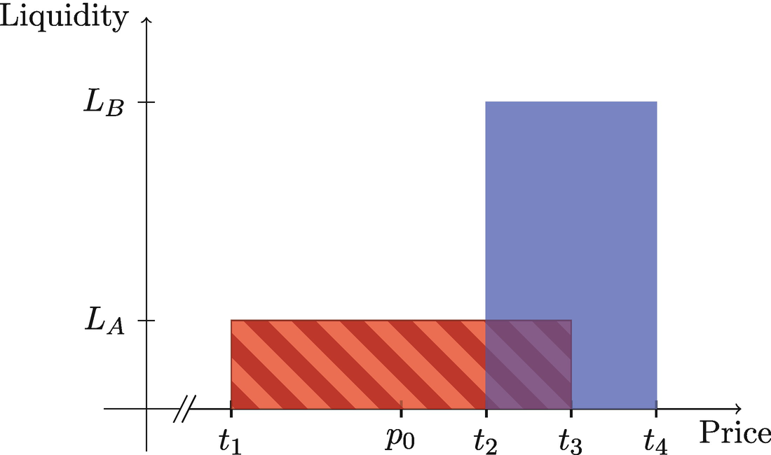
Note that the initialized ticks are t₁, t₂, t₃, and t₄ and that the current price p₀ = 3,800 belongs to [t₁, t₂]. Note also that the liquidity of the pool in the interval [t₁, t₂] is equal to L_A. We depict the situation in Figure 5-11.

Figure 5-11
Representation of the positions of the example

Trade 1. Suppose that a trader wants to buy 1 ETH from the pool. By Equation 5.4, the virtual balances of the pool at the current price p₀(3,800) are

${x}_v=frac{L_A}{sqrt{p_0}}approx 118.62765kern1em extrm{and}kern1em {y}_v={L}_Asqrt{p_0}approx 450,785.07922.$

In addition, from Table 5-1, we obtain that the real balance of ETH at the current price (within the interval [t₁, t₂]) is

${x}_r={L}_Aleft(frac{1}{sqrt{3800}}-frac{1}{sqrt{t_2}} ight)approx 1.528.$

Since the trader wants to buy 1 ETH and x_r > 1, it follows that the trade can be completed within the interval [t₁, t₂].

From Equation 2.8, we obtain that the amount of USDC that the trader has to deposit in order to receive 1 ETH is

${b}_0=frac{1cdot {y}_v}{left(1-phi ight)left({x}_v-1 ight)}approx 3843.83684$

After the trade, the spot price is updated as

${p}_1={left(frac{L_A}{x_v-1} ight)}^2approx 3864.8853.$

Note that 3,864.8853 ∈ [t₁, t₂].

In addition, the trading fee of this trade is 0.3% of the amount that goes into the pool, and hence, it is approximately

Thus,

${f}_g^1=frac{11.53151}{L_A}approx 0.0015769.$

Clearly, ${f}_g^0=0$ and also ${f}_o^jleft({i}_k ight)=0$ for all j ∈ {0, 1} and for all k ∈ {1,2,3,4}.

Trade 2. Suppose now that another trader wants to deposit 5,000 USDC into the pool in order to buy ETH.

Following the analysis of Case 4 of the previous subsection, let y_r be the real balance of USDC within the interval [t₁, t₂] and let y_max be the maximum possible value of the real balance of USDC in the same interval. From Table 5-1, we know that

${y}_r={L}_Aleft(sqrt{p_1}-sqrt{t_1} ight)approx 15855.0899$

and

${y}_{ extrm{max}}={L}_Aleft(sqrt{t_2}-sqrt{t_1} ight)approx 17905.3157.$

Since

${y}_r+5000cdot left(1-phi ight)approx 20840.0899>{y}_{ extrm{max}}$

the trade cannot be completed within the interval [t₁, t₂]. Thus, a first step of the trade is performed, trading an amount ${b}_1^{hbox{'}}$ of USDC where

${b}_1^{hbox{'}}={y}_{ extrm{max}}-{y}_rapprox 2050.2258.$

Note that this value of ${b}_1^{hbox{'}}$ is obtained from the equations of the Uniswap v3 protocol, where fees are not considered, since they are separated and kept aside. Hence, in order to have an amount ${b}_1^{hbox{'}}$ of USDC to trade (without fees being charged to it), the trader must provide an amount b₁ of USDC such that $0.997{b}_1={b}_1^{hbox{'}}$ . Then, the fee that is charged to the trader in this first step is

$0.003{b}_1=frac{0.003{b}_1^{hbox{'}}}{0.997}approx 6.1692 extrm{USDC}.$

Thus, the updated value of the variable ${f}_g^1$ is

${f}_g^1approx 0.0015769+frac{6.1692}{L_A}approx 0.0024205$

(see Table 5-4).

Table 5-4

Summary of price movements and update of fee variables in trades 1 and 2

	Trade 1	Trade 2
	Trade 1	Step 1	Tick cross	Step 2
Price	p₀ → p₁	p₁ → t₂	t₂	t₂ → p₃
Fee	11.53151	6.1692	0	8.8308
${f}_g^1$	0.0015769	0.0024205	0.0024205	0.0026913
${f}_o^1left({i}_2 ight)$	0	0	0.0024205	0.0024205
${f}_a^1left({i}_2 ight)$	0	0	0	0.0002708
${f}_b^1left({i}_2 ight)$	0.0015769	0.0024205	0.0024205	0.0024205

The amount a₁ of ETH that the trader receives for the first step of the trade can be computed using Equation 2.3 (since the fee is charged separately) with the updated virtual balances. We obtain that

${a}_1=frac{left({x}_v-1 ight){b}_1^{hbox{'}}}{left({y}_v+{b}_0^{hbox{'}} ight)+{b}_1^{hbox{'}}}approx 0.528.$

However, since the Uniswap v3 smart contract does not track the virtual balances, we will compute the amount a₁ in a different way. Observe that the virtual balances of the pool at the current price p₁ are

${x}_v=frac{L_A}{sqrt{p_1}}approx 117.62765; extrm{and}kern1em {y}_v={L}_Asqrt{p_1}approx 454,617.3845.$

After the first step of the trade, the updated virtual balance of USDC will be

${y}_v^{hbox{'}}={y}_v+{b}_1^{hbox{'}}approx 456,667.6103$

and hence, the updated price will be

${p}^{hbox{'}}={left(frac{y_v^{hbox{'}}}{L_A} ight)}^2approx 3899.823492$

that is, p^' = t₂, as expected. The virtual balance of ETH at price t₂ (with respect to the interval [t₁, t₂]) is

${x}_v^{hbox{'}}=frac{L_A}{sqrt{t_2}}approx 117.09956.$

The difference between the virtual balances of ETH at prices p₁ and t₂ is the amount of ETH that the trader receives for the first step of the trade, that is,

${a}_1={x}_v-{x}_v^{hbox{'}}approx 0.528.$

Now, note that the amount to be traded is 5,000 USDC, which is greater than the amount b₁ used in the first step, since

${b}_1=frac{b_1^{hbox{'}}}{0.997}approx 2056.395.$

Hence, tick t₂ needs to be crossed, and the remaining amount of USDC, which is 5,000 − b₁ ≈ 2,943.605, is going to be traded in the interval [t₂, t₃]. Before carrying out the second part of the trade, recall that the variables ${L}_{ extrm{tot}},{f}_o^0left({i}_2 ight)$ , and ${f}_o^1left({i}_2 ight)$ are updated since tick t₂ is crossed. Observe that the updated values of these variables are

${displaystyle egin{array}{ll}{L}_{ extrm{tot}}& ={L}_A+{L}_B\ {}{f}_o^0left({i}_2 ight)& ={f}_g^0-{f}_o^0left({i}_2 ight)=0-0=0, extrm{and}\ {}{f}_o^1left({i}_2 ight)& ={f}_g^1-{f}_o^1left({i}_2 ight)=0.0024205-0=0.0024205end{array}}$

(see Table 5-4).

Now we will perform the second part of the trade. Let b₂ be the remaining amount of USDC to be traded. As we pointed out before, b₂ ≈ 2,943.605. Note that the current price is t₂ and that the real balance of USDC at price t₂ with respect to the interval [t₂, t₃] is 0 (by the formulae of Table 5-1). Let ${y}_{ extrm{max}}^{hbox{'}}$ be the maximum possible value of the real balance of USDC in the interval [t₂, t₃]. From Table 5-1, we obtain that

${y}_{ extrm{max}}^{hbox{'}}=left({L}_A+{L}_B ight)left(sqrt{t_3}-sqrt{t_2} ight)approx 25920.9386.$

Let

${b}_2^{hbox{'}}=left(1-phi ight){b}_2=0.997{b}_2approx 2934.774.$

Since ${b}_2^{hbox{'}}$ is clearly smaller than ${y}_{ extrm{max}}^{hbox{'}}$ , the second step of the trade can be completed within the interval [t₂, t₃]. Note that ${b}_2^{hbox{'}}$ is the amount to be actually deposited in the pool and traded for ETH.

The fee that is charged in the second part of the trade is

$0.003{b}_2approx 2943.605cdot 0.003approx 8.8308 extrm{USDC}$

and hence, the updated value of the variable ${f}_g^1$ is

${f}_g^1approx 0.0024205+frac{8.8308}{L_A+{L}_B}approx 0.0026913.$

Let x_v and y_v be the virtual balances of ETH and USDC, respectively, at the current price t₂ (in the interval [t₂, t₃]). By Equation 5.4,

${x}_v=frac{L_A+{L}_B}{sqrt{t_2}}approx 522.1404$

and

${y}_v=left({L}_A+{L}_B ight)sqrt{t_2}approx 2,036,255.3611.$

After the trade, the updated virtual balance of USDC is

${y}_v^{hbox{'}}={y}_v+{b}_2^{hbox{'}}approx 2,039,190.1352,$

and thus, the updated price is

${p}_3={left(frac{y_v^{hbox{'}}}{L_A+{L}_B} ight)}^2approx 3911.0729.$

Note that 3,911.0729 ∈ [t₂, t₃]. Hence, the updated virtual balance of ETH is

${x}_v^{hbox{'}}=frac{L_A+{L}_B}{sqrt{p_3}}approx 521.3889.$

Let a₂ be the amount of ETH that the trader receives in the second step. Note that

${a}_2={x}_v-{x}_v^{hbox{'}}approx 522.1404-521.3889=0.7515.$

Therefore, the trader receives in total

${a}_1+{a}_2approx 0.528+0.7515=1.2795 ETH.$

In Table 5-4, we summarize the price movements, the amounts of fees charged, and how the variables ${f}_g^1,{f}_o^1left({i}_2 ight),{f}_a^1left({i}_2 ight)$ , and ${f}_b^1left({i}_2 ight)$ are updated in the trades that were analyzed before. The values that are updated in each step are highlighted in bold type.

Collected fees and impermanent loss. We will now compute the amount of fees that each liquidity provider has obtained and find out whether they are facing an impermanent loss or not.

Note that the fees were all charged in USDC. Hence, we will only compute the amount of collected fees in this asset. The amount of fees that liquidity provider A has collected is

${displaystyle egin{array}{ll}{L}_A{f}_r^1left({t}_1,{t}_3 ight)& ={L}_Aleft({f}_g^1-{f}_b^1left({i}_1 ight)-{f}_a^1left({i}_3 ight) ight)\ {}& ={L}_Aleft({f}_g^1-{f}_o^1left({i}_1 ight)-{f}_o^1left({i}_3 ight) ight)\ {}& ={L}_Aleft({f}_g^1-0-0 ight)approx 19.68,end{array}}$

where the second equality follows from the fact that t₁ < p₃ < t₃.

On the other hand, the amount of fees that liquidity provider B has collected is

${displaystyle egin{array}{ll}{L}_B{f}_r^1left({t}_2,{t}_4 ight)& ={L}_Bleft({f}_g^1-{f}_b^1left({i}_2 ight)-{f}_a^1left({i}_4 ight) ight)\ {}& ={L}_Bleft({f}_g^1-{f}_o^1left({i}_2 ight)-{f}_o^1left({i}_4 ight) ight)\ {}& ={L}_Bleft({f}_g^1-{f}_o^1left({i}_2 ight)-0 ight)approx 6.85,end{array}}$

where the second equality follows from the fact that t₂ < p₃ < t₄.

We will now analyze the existence of impermanent losses. Recall that liquidity provider A deposited 3 ETH and a certain amount of USDC when the price was 3,800 and the liquidity parameter of their position was L_A ≈ 7,312.6996. From Table 5-1, we obtain that the amount of USDC that they had to deposit was

${L}_Aleft(sqrt{3800}-sqrt{t_1} ight)approx 12,022.78454.$

Hence, if they had never deposited their assets into the pool, the value of their position at the current price p₃ would have been

${V}_Aapprox 3cdot {p}_3+12,022.78454approx 23756 extrm{USDC}.$

On the other hand, applying the formulae of Table 5-1, we obtain that the real balances of their position (at the current price p₃) are

${L}_Aleft(frac{1}{sqrt{p_3}}-frac{1}{sqrt{t_3}} ight)approx 1.303378 ETH.$

and

${L}_Aleft(sqrt{p_3}-sqrt{t_1} ight)approx 18,563.49259 extrm{USDC}.$

Hence, the current value of their position is

${V}_A^{hbox{'}}approx 1.303378{p}_3+18,563.49259approx 23661.1 extrm{USDC}.$

Therefore, liquidity provider A is facing an impermanent loss of approximately 23,756 − 23,661.1 = 94.9 USDC, which is not compensated by the fees of 19.68 USDC they have earned.

On the other hand, liquidity provider B deposited 10 ETH into the pool (and 0 USDC, since the price at the moment of the deposit was below the interval they chose). If they had never deposited that amount of ETH into the pool, the value of their position at the current price of p₃ would have been

${V}_Bapprox 10cdot {p}_3approx 39110.73 extrm{USDC}.$

From Table 5-1, we get that at price p₃, the real balances of their position are

${L}_Bleft(frac{1}{sqrt{p_3}}-frac{1}{sqrt{t_4}} ight)approx 9.4170708 ETH.$

and

${L}_Bleft(sqrt{p_3}-sqrt{t_2} ight)approx 2276.59725 extrm{USDC}.$

Hence, the current value of their position is

${V}_B^{hbox{'}}approx 9.4170708{p}_3+2276.59725approx 39,107.45 extrm{USDC}.$

Therefore, liquidity provider B is facing an impermanent loss of approximately 39,110.73 − 39,107.45 = 3.28 USDC, which, in this case, is compensated by the fees of 6.85 USDC they have earned. Observe that the impermanent loss for liquidity provider B is very small because the amounts of ETH and USDC that their position currently has are very similar to those of their original deposit. This is so because although they entered the position at a price of 3,800, they provided liquidity in the interval [t₂, t₄] (which is approximately [3,900, 4,100]), and hence, their position did not change when the price moved from 3,800 to 3,900 (neither did they earn any trading fees). Note that the current price is p₃ ≈ 3,911.0729, which is very near t₂ ≈ 3,900.

5.6 LP Tokens

Unlike Uniswap v2, LP tokens in Uniswap v3 are nonfungible tokens (NFTs) since positions are highly customizable and will be, in general, very different for different liquidity providers. When a liquidity provider adds liquidity to a specific price range, a unique NFT defining the position is minted. Recall that in Uniswap v3, a liquidity provider’s position consists of the address of the owner, the lower tick index, and the upper tick index. These last two define the boundaries of the interval in which the liquidity provider deposited liquidity. The owner of the NFT that represents a certain position can modify that position or redeem the corresponding tokens.

Recall also that each position stores several variables, as we can see in Listing 5-11.⁴

/// @title Position

/// @notice Positions represent an owner address'

↪liquidity between a lower and upper tick boundary

/// @dev Positions store additional state for tracking

↪fees owed to the position

library Position {

// info stored for each user's position

struct Info {

// the amount of liquidity owned by this

↪position

uint128 liquidity;

// fee growth per unit of liquidity as of the

↪last update to liquidity or fees owed

uint256 feeGrowthInside0LastX128;

uint256 feeGrowthInside1LastX128;

// the fees owed to the position owner in

↪token0/token1

uint128 tokensOwed0;

uint128 tokensOwed1;

}

/// @notice Returns the Info struct of a position,

↪given an owner and position boundaries

/// @param self The mapping containing all user

↪positions

/// @param owner The address of the position owner

/// @param tickLower The lower tick boundary of the

↪position

/// @param tickUpper The upper tick boundary of the

↪position

/// @return position The position info struct of

↪the given owners' position

function get(

mapping(bytes32 => Info) storage self,

address owner,

int24 tickLower,

int24 tickUpper

) internal view returns (Position.Info storage

↪position) {

position =

↪self[keccak256(abi.encodePacked(owner, tickLower,

↪tickUpper))];

}

/// @notice Credits accumulated fees to a user's

↪position

/// @param self The individual position to update

/// @param liquidityDelta The change in pool

↪liquidity as a result of the position update

/// @param feeGrowthInside0X128 The all-time fee

↪growth in token0, per unit of liquidity, inside the

↪position's tick boundaries

/// @param feeGrowthInside1X128 The all-time fee

↪growth in token1, per unit of liquidity, inside the

↪position's tick boundaries

function update(

Info storage self,

int128 liquidityDelta,

uint256 feeGrowthInside0X128,

uint256 feeGrowthInside1X128

) internal {

Info memory _self = self;

uint128 liquidityNext;

if (liquidityDelta == 0) {

require(_self.liquidity > 0, 'NP'); //

↪disallow pokes for 0 liquidity positions

liquidityNext = _self.liquidity;

} else {

liquidityNext =

↪LiquidityMath.addDelta(_self.liquidity,

↪liquidityDelta);

}

// calculate accumulated fees

uint128 tokensOwed0 =

uint128(

FullMath.mulDiv(

feeGrowthInside0X128 -

↪_self.feeGrowthInside0LastX128,

_self.liquidity,

FixedPoint128.Q128

)

);

uint128 tokensOwed1 =

uint128(

FullMath.mulDiv(

feeGrowthInside1X128 -

↪_self.feeGrowthInside1LastX128,

_self.liquidity,

FixedPoint128.Q128

)

);

// update the position

if (liquidityDelta != 0) self.liquidity =

↪liquidityNext;

self.feeGrowthInside0LastX128 =

↪feeGrowthInside0X128;

self.feeGrowthInside1LastX128 =

↪feeGrowthInside1X128;

if (tokensOwed0 > 0 || tokensOwed1 > 0) {

// overflow is acceptable, have to withdraw

↪before you hit type(uint128).max fees

self.tokensOwed0 += tokensOwed0;

self.tokensOwed1 += tokensOwed1;

}

Listing 5-11

Position library of the smart contract of Uniswap v3

We also point out that the Position class has two methods: get and update, as we could see in the previous code. The get method returns the Info struct of a position, while the update method credits the accumulated fees to a position and, if necessary, updates the liquidity parameter of that position.

5.6.1 Minting LP Tokens

The input requirements when adding liquidity to the pool—that is, when LP tokens are going to be minted—are the owner, the liquidity added, and the price range defined by the lower and upper tick indexes. The function that is called to perform a new liquidity deposit is the mint function given in Listing 5-12.⁵

/// @inheritdoc IUniswapV3PoolActions

/// @dev noDelegateCall is applied indirectly via

↪_modifyPosition

function mint(

address recipient,

int24 tickLower,

int24 tickUpper,

uint128 amount,

bytes calldata data

) external override lock returns (uint256 amount0,

↪uint256 amount1) {

require(amount > 0);

(, int256 amount0Int, int256 amount1Int) =

_modifyPosition(

ModifyPositionParams({

owner: recipient,

tickLower: tickLower,

tickUpper: tickUpper,

liquidityDelta:

↪int256(amount).toInt128()

})

);

amount0 = uint256(amount0Int);

amount1 = uint256(amount1Int);

uint256 balance0Before;

uint256 balance1Before;

if (amount0 > 0) balance0Before = balance0();

if (amount1 > 0) balance1Before = balance1();

↪IUniswapV3MintCallback(msg.sender).uniswapV3MintCallback(amount0

↪amount1, data);

if (amount0 > 0)

↪require(balance0Before.add(amount0) <= balance0(),

↪'M0');

if (amount1 > 0)

↪require(balance1Before.add(amount1) <= balance1(),

↪'M1');

emit Mint(msg.sender, recipient, tickLower,

↪tickUpper, amount, amount0, amount1);

}

Listing 5-12

mint function of the smart contract of Uniswap v3

5.6.2 Modifying the Position: Part I

One of the most important parts of the mint function is the function _modifyPosition, which creates a new position and allows the owner to modify it. The parameters that are needed in order to modify the position are the owner, the tick range, and the liquidity that is going to be added or removed. This is shown in Listing 5-13.

struct ModifyPositionParams {

// the address that owns the position

address owner;

// the lower and upper tick of the position

int24 tickLower;

int24 tickUpper;

// any change in liquidity

int128 liquidityDelta;

}

Listing 5-13

Parameters needed to modify a position

The position is updated using the previous parameters, as we can see in Listing 5-14, where the _updatePosition function is called.

/// @dev Effect some changes to a position

/// @param params the position details and the

↪change to the position's liquidity to effect

/// @return position a storage pointer referencing

↪the position with the given owner and tick range

/// @return amount0 the amount of token0 owed to

↪the pool, negative if the pool should pay the

↪recipient

/// @return amount1 the amount of token1 owed to

↪the pool, negative if the pool should pay the

↪recipient

function _modifyPosition(ModifyPositionParams

↪memory params)

private

noDelegateCall

returns (

Position.Info storage position,

int256 amount0,

int256 amount1

)

{

checkTicks(params.tickLower, params.tickUpper);

Slot0 memory _slot0 = slot0; // SLOAD for gas

↪optimization

position = _updatePosition(

params.owner,

params.tickLower,

params.tickUpper,

params.liquidityDelta,

_slot0.tick

);

...

Listing 5-14

First part of the _modifyPosition function of the smart contract of Uniswap v3

5.6.3 Update the Position

The function _updatePosition, shown in Listing 5-15, updates the liquidity of the position and computes and stores the accumulated fees since the last update, as we can see in the following code. It also initializes or uninitializes the boundary tick indexes of the position in case either of these actions is needed (e.g., if the position is created or removed and the boundary tick indexes are not referenced by any other position).

/// @dev Gets and updates a position with the given

↪liquidity delta

/// @param owner the owner of the position

/// @param tickLower the lower tick of the

↪position's tick range

/// @param tickUpper the upper tick of the

↪position's tick range

/// @param tick the current tick, passed to avoid

↪sloads

function _updatePosition(

address owner,

int24 tickLower,

int24 tickUpper,

int128 liquidityDelta,

int24 tick

) private returns (Position.Info storage position)

↪{

position = positions.get(owner, tickLower,

↪tickUpper);

uint256 _feeGrowthGlobal0X128 =

↪feeGrowthGlobal0X128; // SLOAD for gas

↪optimization

uint256 _feeGrowthGlobal1X128 =

↪feeGrowthGlobal1X128; // SLOAD for gas

↪optimization

// if we need to update the ticks, do it

bool flippedLower;

bool flippedUpper;

if (liquidityDelta != 0) {

uint32 time = _blockTimestamp();

(int56 tickCumulative, uint160

↪secondsPerLiquidityCumulativeX128) =

observations.observeSingle(

time,

slot0.tick,

slot0.observationIndex,

liquidity,

slot0.observationCardinality

);

flippedLower = ticks.update(

tickLower,

tick,

liquidityDelta,

_feeGrowthGlobal0X128,

_feeGrowthGlobal1X128,

secondsPerLiquidityCumulativeX128,

tickCumulative,

time,

false,

maxLiquidityPerTick

);

flippedUpper = ticks.update(

tickUpper,

tick,

liquidityDelta,

_feeGrowthGlobal0X128,

_feeGrowthGlobal1X128,

secondsPerLiquidityCumulativeX128,

tickCumulative,

time,

true,

maxLiquidityPerTick

);

if (flippedLower) {

tickBitmap.flipTick(tickLower, tickSpacing);

}

if (flippedUpper) {

tickBitmap.flipTick(tickUpper, tickSpacing);

}

(uint256 feeGrowthInside0X128, uint256

↪feeGrowthInside1X128) =

ticks.getFeeGrowthInside(tickLower,

↪tickUpper, tick, _feeGrowthGlobal0X128,

↪_feeGrowthGlobal1X128);

position.update(liquidityDelta,

↪feeGrowthInside0X128, feeGrowthInside1X128);

// clear any tick data that is no longer

↪needed

if (liquidityDelta < 0) {

if (flippedLower) {

ticks.clear(tickLower);

}

if (flippedUpper) {

ticks.clear(tickUpper);

}

Listing 5-15

_updatePosition function of the smart contract of Uniswap v3

5.6.4 Tick Class

In the previous code, the Tick class⁶ appeared. Its code is given in Listing 5-16. Observe that the Tick class keeps track of the following variables:

liquidityGross
liquidityNet
feeGrowth0utside0X128
feeGrowth0utside1X128

which, in the previous section, were denoted by ${L}_g,Delta L,{f}_o^0$ , and ${f}_o^1$ , respectively. Note also that the method getFeeGrowthInside defines the following variables:

feeGrowthBelow0X128
feeGrowthBelow 1X128
feegrowthAbove0X128
feegrowthAbove 1X128
feeGrowthInside0X128
feeGrowthInside1X128

which correspond to the variables ${f}_b^0,{f}_b^1,{f}_a^0,{f}_a^1,{f}_r^0$ , and ${f}_r^1$ , respectively, that were defined in the previous section.

/// @title Tick

/// @notice Contains functions for managing tick

↪processes and relevant calculations

library Tick {

using LowGasSafeMath for int256;

using SafeCast for int256;

// info stored for each initialized individual

↪tick

struct Info {

// the total position liquidity that references

↪this tick

uint128 liquidityGross;

// amount of net liquidity added (subtracted)

↪when tick is crossed from left to right (right to

↪left),

int128 liquidityNet;

// fee growth per unit of liquidity on the

↪_other_ side of this tick (relative to the current

↪tick)

// only has relative meaning, not absolute -

↪the value depends on when the tick is initialized

uint256 feeGrowthOutside0X128;

uint256 feeGrowthOutside1X128;

// the cumulative tick value on the other side

↪of the tick

int56 tickCumulativeOutside;

// the seconds per unit of liquidity on the

↪_other_ side of this tick (relative to the current

↪tick)

// only has relative meaning, not absolute -

↪the value depends on when the tick is initialized

uint160 secondsPerLiquidityOutsideX128;

// the seconds spent on the other side of the

↪tick (relative to the current tick)

// only has relative meaning, not absolute -

↪the value depends on when the tick is initialized

uint32 secondsOutside;

// true iff the tick is initialized, i.e. the

↪value is exactly equivalent to the expression

↪liquidityGross != 0

// these 8 bits are set to prevent fresh

↪sstores when crossing newly initialized ticks

bool initialized;

}

/// @notice Derives max liquidity per tick from

↪given tick spacing

/// @dev Executed within the pool constructor

/// @param tickSpacing The amount of required tick

↪separation, realized in multiples of `tickSpacing`

/// e.g., a tickSpacing of 3 requires ticks to

↪be initialized every 3rd tick i.e., ..., -6, -3, 0,

↪3, 6, ...

/// @return The max liquidity per tick

function tickSpacingToMaxLiquidityPerTick(int24

↪tickSpacing) internal pure returns (uint128) {

int24 minTick = (TickMath.MIN_TICK /

↪tickSpacing) * tickSpacing;

int24 maxTick = (TickMath.MAX_TICK /

↪tickSpacing) * tickSpacing;

uint24 numTicks = uint24((maxTick - minTick) /

↪tickSpacing) + 1;

return type(uint128).max / numTicks;

}

/// @notice Retrieves fee growth data

/// @param self The mapping containing all tick

↪information for initialized ticks

/// @param tickLower The lower tick boundary of the

↪position

/// @param tickUpper The upper tick boundary of the

↪position

/// @param tickCurrent The current tick

/// @param feeGrowthGlobal0X128 The all-time global

↪fee growth, per unit of liquidity, in token0

/// @param feeGrowthGlobal1X128 The all-time global

↪fee growth, per unit of liquidity, in token1

/// @return feeGrowthInside0X128 The all-time fee

↪growth in token0, per unit of liquidity, inside the

↪position's tick boundaries

/// @return feeGrowthInside1X128 The all-time fee

↪growth in token1, per unit of liquidity, inside the

↪position's tick boundaries

function getFeeGrowthInside(

mapping(int24 => Tick.Info) storage self,

int24 tickLower,

int24 tickUpper,

int24 tickCurrent,

uint256 feeGrowthGlobal0X128,

uint256 feeGrowthGlobal1X128

) internal view returns (uint256

↪feeGrowthInside0X128, uint256 feeGrowthInside1X128)

↪{

Info storage lower = self[tickLower];

Info storage upper = self[tickUpper];

// calculate fee growth below

uint256 feeGrowthBelow0X128;

uint256 feeGrowthBelow1X128;

if (tickCurrent >= tickLower) {

feeGrowthBelow0X128 =

↪lower.feeGrowthOutside0X128;

feeGrowthBelow1X128 =

↪lower.feeGrowthOutside1X128;

} else {

feeGrowthBelow0X128 = feeGrowthGlobal0X128

↪– lower.feeGrowthOutside0X128;

feeGrowthBelow1X128 = feeGrowthGlobal1X128

↪– lower.feeGrowthOutside1X128;

}

// calculate fee growth above

uint256 feeGrowthAbove0X128;

uint256 feeGrowthAbove1X128;

if (tickCurrent < tickUpper) {

feeGrowthAbove0X128 =

↪upper.feeGrowthOutside0X128;

feeGrowthAbove1X128 =

↪upper.feeGrowthOutside1X128;

} else {

feeGrowthAbove0X128 = feeGrowthGlobal0X128

↪- upper.feeGrowthOutside0X128;

feeGrowthAbove1X128 = feeGrowthGlobal1X128

↪- upper.feeGrowthOutside1X128;

}

feeGrowthInside0X128 = feeGrowthGlobal0X128 -

↪feeGrowthBelow0X128 - feeGrowthAbove0X128;

feeGrowthInside1X128 = feeGrowthGlobal1X128 -

↪feeGrowthBelow1X128 - feeGrowthAbove1X128;

}

/// @notice Updates a tick and returns true if the

↪tick was flipped from initialized to uninitialized,

↪or vice versa

/// @param self The mapping containing all tick

↪information for initialized ticks

/// @param tick The tick that will be updated

/// @param tickCurrent The current tick

/// @param liquidityDelta A new amount of liquidity

↪to be added (subtracted) when tick is crossed from

↪left to right (right to left)

/// @param feeGrowthGlobal0X128 The all-time global

↪fee growth, per unit of liquidity, in token0

/// @param feeGrowthGlobal1X128 The all-time global

↪fee growth, per unit of liquidity, in token1

/// @param secondsPerLiquidityCumulativeX128 The

↪all-time seconds per max(1, liquidity) of the pool

/// @param tickCumulative The tick * time elapsed

↪since the pool was first initialized

/// @param time The current block timestamp cast to

↪a uint32

/// @param upper true for updating a position's

↪upper tick, or false for updating a position's

↪lower tick

/// @param maxLiquidity The maximum liquidity

↪allocation for a single tick

/// @return flipped Whether the tick was flipped

↪from initialized to uninitialized, or vice versa

function update(

mapping(int24 => Tick.Info) storage self,

int24 tick,

int24 tickCurrent,

int128 liquidityDelta,

uint256 feeGrowthGlobal0X128,

uint256 feeGrowthGlobal1X128,

uint160 secondsPerLiquidityCumulativeX128,

int56 tickCumulative,

uint32 time,

bool upper,

uint128 maxLiquidity

) internal returns (bool flipped) {

Tick.Info storage info = self[tick];

uint128 liquidityGrossBefore =

↪info.liquidityGross;

uint128 liquidityGrossAfter =

↪LiquidityMath.addDelta(liquidityGrossBefore,

↪liquidityDelta);

require(liquidityGrossAfter <= maxLiquidity,

↪'LO');

flipped = (liquidityGrossAfter == 0) !=

↪(liquidityGrossBefore == 0);

if (liquidityGrossBefore == 0) {

// by convention, we assume that all growth

↪before a tick was initialized happened _below_ the

↪tick

if (tick <= tickCurrent) {

info.feeGrowthOutside0X128 =

↪feeGrowthGlobal0X128;

info.feeGrowthOutside1X128 =

↪feeGrowthGlobal1X128;

info.secondsPerLiquidityOutsideX128 =

↪secondsPerLiquidityCumulativeX128;

info.tickCumulativeOutside =

↪tickCumulative;

info.secondsOutside = time;

}

info.initialized = true;

}

info.liquidityGross = liquidityGrossAfter;

// when the lower (upper) tick is crossed left

↪to right (right to left), liquidity must be added

↪(removed)

info.liquidityNet = upper

↪int256(info.liquidityNet).sub(liquidityDelta).toInt128()

↪int256(info.liquidityNet).add(liquidityDelta).toInt128();

}

/// @notice Clears tick data

/// @param self The mapping containing all

↪initialized tick information for initialized ticks

/// @param tick The tick that will be cleared

function clear(mapping(int24 => Tick.Info) storage

↪self, int24 tick) internal {

delete self[tick];

}

/// @notice Transitions to next tick as needed by

↪price movement

/// @param self The mapping containing all tick

↪information for initialized ticks

/// @param tick The destination tick of the

↪transition

/// @param feeGrowthGlobal0X128 The all-time global

↪fee growth, per unit of liquidity, in token0

/// @param feeGrowthGlobal1X128 The all-time global

↪fee growth, per unit of liquidity, in token1

/// @param secondsPerLiquidityCumulativeX128 The

↪current seconds per liquidity

/// @param tickCumulative The tick * time elapsed

↪since the pool was first initialized

/// @param time The current block.timestamp

/// @return liquidityNet The amount of liquidity

↪added (subtracted) when tick is crossed from left

↪to right (right to left)

function cross(

mapping(int24 => Tick.Info) storage self,

int24 tick,

uint256 feeGrowthGlobal0X128,

uint256 feeGrowthGlobal1X128,

uint160 secondsPerLiquidityCumulativeX128,

int56 tickCumulative,

uint32 time

) internal returns (int128 liquidityNet) {

Tick.Info storage info = self[tick];

info.feeGrowthOutside0X128 =

↪feeGrowthGlobal0X128 - info.feeGrowthOutside0X128;

info.feeGrowthOutside1X128 =

↪feeGrowthGlobal1X128 - info.feeGrowthOutside1X128;

info.secondsPerLiquidityOutsideX128 =

↪secondsPerLiquidityCumulativeX128 -

↪info.secondsPerLiquidityOutsideX128;

info.tickCumulativeOutside = tickCumulative -

↪info.tickCumulativeOutside;

info.secondsOutside = time -

↪info.secondsOutside;

liquidityNet = info.liquidityNet;

}

Listing 5-16

Tick class of the smart contract of Uniswap v3

Modifying the Position: Part II

The second part of the _modifyPosition function computes the amounts of each of the pool tokens that the liquidity provider needs to deposit in order to set up the position. These amounts are called amount0 and amount1 and are returned by the _modifyPosition function. Recall that the formulae for computing these amounts are given in Table 5-1. We show the whole _modifyPosition function in Listing 5-17.

/// @dev Effect some changes to a position

/// @param params the position details and the

↪change to the position's liquidity to effect

/// @return position a storage pointer referencing

↪the position with the given owner and tick range

/// @return amount0 the amount of token0 owed to

↪the pool, negative if the pool should pay the

↪recipient

/// @return amount1 the amount of token1 owed to

↪the pool, negative if the pool should pay the

↪recipient

function _modifyPosition(ModifyPositionParams

↪memory params)

private

noDelegateCall

returns (

Position.Info storage position,

int256 amount0,

int256 amount1

)

{

checkTicks(params.tickLower, params.tickUpper);

Slot0 memory _slot0 = slot0; // SLOAD for gas

↪optimization

position = _updatePosition(

params.owner,

params.tickLower,

params.tickUpper,

params.liquidityDelta,

_slot0.tick

);

if (params.liquidityDelta != 0) {

if (_slot0.tick < params.tickLower) {

// current tick is below the passed

↪range; liquidity can only become in range by

↪crossing from left to

// right, when we'll need _more_ token0

↪(it's becoming more valuable) so user must provide

↪it

amount0 =

↪SqrtPriceMath.getAmount0Delta(

↪TickMath.getSqrtRatioAtTick(params.tickLower),

↪TickMath.getSqrtRatioAtTick(params.tickUpper),

params.liquidityDelta

);

} else if (_slot0.tick < params.tickUpper)

↪{

// current tick is inside the passed

↪range

uint128 liquidityBefore = liquidity; //

↪SLOAD for gas optimization

// write an oracle entry

(slot0.observationIndex,

↪slot0.observationCardinality) = observations.write(

_slot0.observationIndex,

_blockTimestamp(),

_slot0.tick,

liquidityBefore,

_slot0.observationCardinality,

_slot0.observationCardinalityNext

);

amount0 =

↪SqrtPriceMath.getAmount0Delta(

_slot0.sqrtPriceX96,

↪TickMath.getSqrtRatioAtTick(params.tickUpper),

params.liquidityDelta

);

amount1 =

↪SqrtPriceMath.getAmount1Delta(

↪TickMath.getSqrtRatioAtTick(params.tickLower),

_slot0.sqrtPriceX96,

params.liquidityDelta

);

liquidity =

↪LiquidityMath.addDelta(liquidityBefore,

↪params.liquidityDelta);

} else {

// current tick is above the passed

↪range; liquidity can only become in range by

↪crossing from right to

// left, when we'll need _more_ token1

↪(it's becoming more valuable) so user must provide

↪it

amount1 =

↪SqrtPriceMath.getAmount1Delta(

↪TickMath.getSqrtRatioAtTick(params.tickLower),

↪TickMath.getSqrtRatioAtTick(params.tickUpper),

params.liquidityDelta

);

}

Listing 5-17

_modifyPosition function of the smart contract of Uniswap v3

Observe that the previous code uses the functions getAmount0Delta and getAmount1Delta from the SqrtPriceMath library.⁷ These functions are given in Listing 5-18.

/// @notice Gets the amount0 delta between two

↪prices

/// @dev Calculates liquidity / sqrt(lower) -

↪liquidity / sqrt(upper),

/// i.e. liquidity * (sqrt(upper) - sqrt(lower)) /

↪(sqrt(upper) * sqrt(lower))

/// @param sqrtRatioAX96 A sqrt price

/// @param sqrtRatioBX96 Another sqrt price

/// @param liquidity The amount of usable

↪liquidity

/// @param roundUp Whether to round the amount up

↪or down

/// @return amount0 Amount of token0 required to

↪cover a position of size liquidity between the two

↪passed prices

function getAmount0Delta(

uint160 sqrtRatioAX96,

uint160 sqrtRatioBX96,

uint128 liquidity,

bool roundUp

) internal pure returns (uint256 amount0) {

if (sqrtRatioAX96 > sqrtRatioBX96)

↪(sqrtRatioAX96, sqrtRatioBX96) = (sqrtRatioBX96,

↪sqrtRatioAX96);

uint256 numerator1 = uint256(liquidity) <<

↪FixedPoint96.RESOLUTION;

uint256 numerator2 = sqrtRatioBX96 -

↪sqrtRatioAX96;

require(sqrtRatioAX96 > 0);

return

roundUp

? UnsafeMath.divRoundingUp(

↪FullMath.mulDivRoundingUp(numerator1, numerator2,

↪sqrtRatioBX96),

sqrtRatioAX96

)

: FullMath.mulDiv(numerator1,

↪numerator2, sqrtRatioBX96) / sqrtRatioAX96;

}

/// @notice Gets the amount1 delta between two

↪prices

/// @dev Calculates liquidity * (sqrt(upper) -

↪sqrt(lower))

/// @param sqrtRatioAX96 A sqrt price

/// @param sqrtRatioBX96 Another sqrt price

/// @param liquidity The amount of usable

↪liquidity

/// @param roundUp Whether to round the amount up,

↪or down

/// @return amount1 Amount of token1 required to

↪cover a position of size liquidity between the two

↪passed prices

function getAmount1Delta(

uint160 sqrtRatioAX96,

uint160 sqrtRatioBX96,

uint128 liquidity,

bool roundUp

) internal pure returns (uint256 amount1) {

if (sqrtRatioAX96 > sqrtRatioBX96)

↪(sqrtRatioAX96, sqrtRatioBX96) = (sqrtRatioBX96,

↪sqrtRatioAX96);

return

roundUp

? FullMath.mulDivRoundingUp(liquidity,

↪sqrtRatioBX96 - sqrtRatioAX96, FixedPoint96.Q96)

: FullMath.mulDiv(liquidity,

↪sqrtRatioBX96 - sqrtRatioAX96, FixedPoint96.Q96);

}

Listing 5-18

Functions getAmount0Delta and getAmount1Delta of the smart contract of Uniswap v3

Observe also that in the code of the _modifyPosition function, the amounts

slot0.sqrtPriceX96 ,

TickMath.getSqrtRatioAtTick(params.tickLower) , and

TickMath.getSqrtRatioAtTick(params.tickUpper)

correspond to the variables $$ sqrt{ extrm{p}},sqrt{pa}, $$ and $$ sqrt{pb} $$ , respectively, that are used in Table 5-1.

5.6.5 Burning LP Tokens

The owner of LP tokens of a Uniswap v3 pool can remove liquidity. The liquidity removal process will burn the LP tokens, remove the position, and give back to the liquidity provider a certain amount of assets, according to the formulae of Table 5-1. In addition, the fees that accumulated since the last time they were collected are given to the liquidity provider.

As we can see in Listing 5-19, the burn function makes use of the _modifyPosition function that we studied before. In this case, a negative value for the liquidity is used, since liquidity is removed instead of being deposited.

/// @inheritdoc IUniswapV3PoolActions

/// @dev noDelegateCall is applied indirectly via

↪_modifyPosition

function burn(

int24 tickLower,

int24 tickUpper,

uint128 amount

) external override lock returns (uint256 amount0,

↪uint256 amount1) {

(Position.Info storage position, int256

↪amount0Int, int256 amount1Int) =

_modifyPosition(

ModifyPositionParams({

owner: msg.sender,

tickLower: tickLower,

tickUpper: tickUpper,

liquidityDelta:

↪– int256(amount).toInt128()

})

);

amount0 = uint256(-amount0Int);

amount1 = uint256(-amount1Int);

if (amount0 > 0 || amount1 > 0) {

(position.tokensOwed0,

↪position.tokensOwed1) = (

position.tokensOwed0 +

↪uint128(amount0),

position.tokensOwed1 + uint128(amount1)

);

}

emit Burn(msg.sender, tickLower, tickUpper,

↪amount, amount0, amount1);

}

Listing 5-19

burn function of the smart contract of Uniswap v3

5.7 Analysis of Liquidity Provisioning

Compared to Uniswap v2, in Uniswap v3, liquidity is provided with higher capital efficiency, meaning that with the same amount of deposited tokens, one can obtain a higher liquidity parameter in the chosen interval. This is beneficial for traders, since the higher the liquidity parameter is, the lower the price impact will be. However, for liquidity providers, the situation is very different. In order to analyze this, we will consider two situations with two different assumptions.

First, suppose that the exact same trades are executed in a Uniswap v2 pool and in a Uniswap v3 pool. In this case, the amount of trading fees collected by both pools will be the same—for example, 0.3% of the incoming amount of each trade—and the total collected fees will be shared between all the liquidity providers. In the Uniswap v2 pool, the fees will be shared in a way that is proportional to the deposits the liquidity providers made, while in the Uniswap v3 pool, this proportion will also depend on the interval that each liquidity provider chose. More explicitly, in the case of the Uniswap v3 pool, as we have seen, the liquidity providers earn fees only for the trades (or portion of trades) that are performed within the interval they chose, and in this case, their share of fees is equal to the liquidity parameter they provided divided by the total liquidity—which will also be higher than in a Uniswap v2 pool. To sum up, comparing a Uniswap v2 pool with a Uniswap v3 pool, if the same trades are performed, the total collected fees will be the same, and thus, liquidity providers will not be able to obtain more fees in general with the Uniswap v3 pool, although it may happen that some of them earn more fees with respect to a Uniswap v2 pool and some of them earn fewer fees.

For the second situation, we will consider a completely different assumption. One can argue that a considerable part of the trades that are executed in a Uniswap pool (either v2 or v3) is done by arbitrageurs and that arbitrageurs have enough money to perform any required trade. Thus, every time the spot price of the pool deviates from the market price, arbitrageurs will step in and make a trade. Due to the concentrated liquidity of Uniswap v3, in the price range that is near the market price, we usually have far more liquidity than in a Uniswap v2 pool. Hence, the arbitrageurs of Uniswap v3 will need to perform a bigger trade to make the spot price equal to the market price, or in other words, they will have the opportunity to make more money with the arbitrage. Since a bigger trade is performed, a larger amount of fees is collected, which may, at first sight, seem beneficial to liquidity providers. However, as we have seen in Section 5.3, concentrated liquidity also implies a higher impermanent loss for liquidity providers in many different possible scenarios. In addition, several analyses show that the possible greater amount of fees that liquidity providers collect (under the assumptions of this paragraph) does not compensate for the higher impermanent losses [25, 33].

5.7.1 Capital Efficiency

In order to compute the amount of liquidity that a liquidity provider puts into a Uniswap v3 pool, we will assume that the entry price is the geometric mean of the boundaries of the interval in which they provide liquidity. Hence, if the current price is p, we will assume that the liquidity provider chooses a price interval [p_a, p_b] such that $sqrt{p_a{p}_b}=p$ . With this assumption, the amounts of each token that are needed to provide liquidity in a Uniswap v3 pool will satisfy the deposit requirements of a Uniswap v2 pool, as we shall see in the following text.

But first note that

$p={p}_asqrt{frac{p_b}{p_a}}kern1em extrm{and}kern1em {p}_b={p}_a{left(sqrt{frac{p_b}{p_a}} ight)}^2.$

This means that if, for example, p is 20% higher than p_a, then p_b is 20% higher than p.

Consider a Uniswap v3 pool of tokens X and Y and let p be the current price of token X in terms of token Y. Suppose that a liquidity provider deposits an amount A₀ of token X and an amount B₀ of token Y in the price interval [p_a, p_b] satisfying that $sqrt{p_a{p}_b}=p$ , and let L be the corresponding liquidity parameter of the position. From Table 5-1, we know that

${A}_0=Lleft(frac{1}{sqrt{p}}-frac{1}{sqrt{p_b}} ight)kern1em extrm{and}kern1em {B}_0=Lleft(sqrt{p}-sqrt{p_a} ight).$

Let

$r=sqrt{frac{p_b}{p_a}}.$

Note that

${p}_a=frac{p}{r}kern1em extrm{and}kern1em {p}_b= rp$

since

${rp}_a=sqrt{frac{p_b}{p_a}}{p}_a=sqrt{p_a{p}_b}=p$

and

$rp=sqrt{frac{p_b}{p_a}}sqrt{p_a{p}_b}={p}_b.$

Now, observe that

$frac{B_0}{A_0}=frac{Lleft(sqrt{p}-sqrt{p_a} ight)}{Lleft(frac{1}{sqrt{p}}-frac{1}{sqrt{p_b}} ight)}=frac{sqrt{p}-frac{sqrt{p}}{sqrt{r}}}{frac{1}{sqrt{p}}-frac{1}{sqrt{p}sqrt{r}}}=frac{sqrt{p}left(1-frac{1}{sqrt{r}} ight)}{frac{1}{sqrt{p}}left(1-frac{1}{sqrt{r}} ight)}=p.$

Hence, since the current price is p, the liquidity provider can deposit an amount A₀ of token X and an amount B₀ of token Y into a Uniswap v2 pool (this follows from Equations 2.4 and 2.12). The liquidity parameter of this Uniswap v2 position is

${L}_2=sqrt{A_0{B}_0}.$

Therefore, the ratio between the liquidity parameters of the Uniswap v3 and Uniswap v2 pools is

${displaystyle egin{array}{ll}frac{L}{L_2}& =frac{L}{sqrt{A_0{B}_0}}=frac{L}{sqrt{Lleft(frac{1}{sqrt{p}}-frac{1}{sqrt{p_b}} ight)Lleft(sqrt{p}-sqrt{p_a} ight)}}\ {}& =frac{1}{sqrt{left(frac{1}{sqrt{p}}-frac{1}{sqrt{r}sqrt{p}} ight)left(sqrt{p}-frac{sqrt{p}}{sqrt{r}} ight)}}\ {}& =frac{1}{sqrt{frac{1}{sqrt{p}}left(1-frac{1}{sqrt{r}} ight)sqrt{p}left(1-frac{1}{sqrt{r}} ight)}}=frac{1}{sqrt{{left(1-frac{1}{sqrt{r}} ight)}^2}}=frac{1}{1-frac{1}{sqrt{r}}}\ {}& =frac{1}{1-{left(frac{p_a}{p_b} ight)}^{frac{1}{4}}}.end{array}}$

Example 5.6. In Table 5-5, we show the (approximate) values of thequotient $frac{L}{L_2}$ for different values of the parameter r together with thecorresponding values of the quotient $frac{p_b}{p_a}$ . For instance, if r = 1.1, thenp_b = 1.21p_a, which means that price p_b is 21% higher that price p_a. In such an interval, the liquidity parameter of a Uniswap v3 position will be approximately 21.5 times higher than the liquidity parameter of the same liquidity deposit into a Uniswap v2 pool.

Table 5-5

Values of the ratios between the liquidity parameters of a Uniswap v3 and a Uniswap v2 position for different values of the parameter r that measures the length of the price interval of Uniswap v3

r	$frac{p_b}{p_a}$	$frac{L}{L_2}$
1.005	1.010025	401.5
1.01	1.0201	201.5
1.05	1.1025	41.5
1.1	1.21	21.5
1.2	1.44	11.5
2	4	3.41
10	100	1.46
100	10,000	1.11

If r = 1.05, then p_b = 1.1025p_a, and hence, p_b is approximately 10% higher than p_a. In this case, the liquidity parameter of a Uniswap v3 position is approximately 41.5 times higher than that of the same deposit into a Uniswap v2 pool. As expected, if the interval in which liquidity is deposited is smaller, then the liquidity parameter will be bigger since if the same amount of tokens is used for trading in a smaller interval, then we can provide more liquidity into that interval.

Of course, we have to remember that if the interval in which the liquidity provider provided liquidity is smaller, then the likelihood of the price falling out of that interval will be greater, and so will be the impermanent loss (see Figure 5-5). In addition, when the price goes out of that interval, the liquidity provider will stop earning trading fees.

5.7.2 Independence with Respect to Other Liquidity Providers

We will now prove that the amount of fees that a liquidity provider earns in a Uniswap v3 pool depends only on the price movement and the parameters that define their position and not on the positions of the other liquidity providers that have deposited liquidity on the same pool. We formalize this statement in the following proposition.

Proposition 5.2. Consider a Uniswap v3 liquidity pool with tokens X and Y and fee ϕ. Suppose that a liquidity provider owns a position in the pool. For each positive real number p, let x_r(p) and y_r(p) be the amount of real reserves at price p of tokens X and Y, respectively, of the liquidity provider’s position.

Let p₁ and p₂ be positive real numbers. Suppose that a single trade in the pool moves the price from p₁ to p₂.

If p₁ < p₂, then the liquidity provider earns an amount

$frac{phi }{1-phi}left({y}_rleft({p}_2 ight)-{y}_rleft({p}_1 ight) ight)$

of token Y in fees.

If p₁ > p₂, then the liquidity provider earns an amount

$frac{phi }{1-phi}left({x}_rleft({p}_2 ight)-{x}_rleft({p}_1 ight) ight)$

of token X in fees.

Proof. By dividing the price movement into several steps, we may assume that the total liquidity of the pool remains constant within the trade. Let L_tot be the total liquidity of the pool corresponding to the interval in which the trade is executed. For each positive real number p, let x_v(p) and y_v(p) be the virtual balances of the pool at price p of tokens X and Y, respectively. Recall that

${x}_v(p)=frac{L_{ extrm{tot}}}{sqrt{p}}kern1em extrm{and}kern1em {y}_v(p)={L}_{ extrm{tot}}sqrt{p}.$

Let L be the liquidity parameter of the liquidity provider’s position, and let [p_a, p_b] be the price interval of the position. For all positive real numbers p, q, let F(p, q) be the amount of trading fees that the liquidity provider’s position earns when the price moves from p to q in a single trade. We will first prove the following assertion, which will be called assertion (A).

(A) For all positive real numbers p, q, if p_a ≤ p < q ≤ p_b, then $Fleft(p,q ight)=frac{phi }{1-phi}left({y}_r(q)-{y}_r(p) ight)$ .

Let p and q be positive real numbers such that p_a ≤ p < q ≤ p_b and suppose that a single trade moves the price from p to q. Since p < q, the amount of token Y in the pool increases, and the amount of token X in the pool decreases. Let b be the amount of token Y that is deposited into the pool. Hence, the trading fee will be charged on this amount b of token Y. Note that the amount of the fee is ϕb, and then the amount of token Y that goes into the pool is (1 − ϕ)b. Thus, y_v(q) = y_v(p) + (1 − ϕ)b. Therefore,

$Fleft(p,q ight)=frac{L}{L_{ extrm{tot}}}phi b=frac{Lphi}{L_{ extrm{tot}}left(1-phi ight)}left({y}_v(q)-{y}_v(p) ight)$

$=frac{Lphi}{L_{ extrm{tot}}left(1-phi ight)}left({L}_{ extrm{tot}}sqrt{q}-{L}_{ extrm{tot}}sqrt{p} ight)=frac{phi }{1-phi}left(Lsqrt{q}-Lsqrt{p} ight)$

$=frac{phi }{1-phi}left(left(Lsqrt{q}-Lsqrt{p_a} ight)-left(Lsqrt{p}-Lsqrt{p_a} ight) ight)$

$=frac{phi }{1-phi}left({y}_r(q)-{y}_r(p) ight),$

where the last equality follows from the formulae of Table 5-1. Hence, we have proved assertion (A).

Now we will prove the following assertion, which will be called assertion (B).

(B) For all positive real numbers p, q, if p_a ≤ q < p ≤ p_b, then $Fleft(p,q ight)=frac{phi }{1-phi}left({x}_r(q)-{x}_r(p) ight)$ .

Let p and q be positive real numbers such that p_a ≤ q < p ≤ p_b and suppose that a single trade moves the price from p to q. Since p > q, the amount of token X in the pool has to increase. Let a be the amount of token X that is deposited into the pool. Hence, the amount of the trading fee is ϕa, and then the amount of token X that goes into the pool is (1 − ϕ)a. Thus, x_v(q) = x_v(p) + (1 − ϕ)a. Therefore,

$Fleft(p,q ight)=frac{L}{L_{ extrm{tot}}}phi a=frac{Lphi}{L_{ extrm{tot}}left(1-phi ight)}left({x}_v(q)-{x}_v(p) ight)$

$=frac{Lphi}{L_{ extrm{tot}}left(1-phi ight)}left(frac{L_{ extrm{tot}}}{sqrt{q}}-frac{L_{ extrm{tot}}}{sqrt{p}} ight)=frac{phi }{1-phi}left(frac{L}{sqrt{q}}-frac{L}{sqrt{p}} ight)$

$=frac{phi }{1-phi}left(left(frac{L}{sqrt{q}}-frac{L}{sqrt{p_b}} ight)-left(frac{L}{sqrt{p}}-frac{L}{sqrt{p_b}} ight) ight)$

$=frac{phi }{1-phi}left({x}_r(q)-{x}_r(p) ight),$

where the last equality follows from the formulae of Table 5-1. Hence, we have proved assertion (B).

We will now prove the first statement of the proposition. Suppose that p₁ < p₂. Since the price increases, an amount of token Y is deposited, and thus, the trading fee is charged on token Y. We will divide our analysis into several cases and subcases.

Case 1: p₁ ≥ p_b.

In this case, p_b ≤ p₁ < p₂, and thus, the price movement is outside the position range. Hence, y_r(p₁) = y_r(p₂), and the amount F(p₁, p₂) of trading fees that the position earns is 0. Observe that

$Fleft({p}_1,{p}_2 ight)=0=frac{phi }{1-phi}left({y}_rleft({p}_2 ight)-{y}_rleft({p}_1 ight) ight),$

that is, the first formula of the statement of the proposition holds.

Case 2: p₂ ≤ p_a.

In this case, p₁ < p₂ ≤ p_a, and hence, the price movement is outside the position range. Then the amount F(p₁, p₂) of trading fees that the position earns is 0. Note that y_r(p₁) = y_r(p₂) = 0 since p₁ < p₂ ≤ p_a. Thus,

$Fleft({p}_1,{p}_2 ight)=0=frac{phi }{1-phi}left({y}_rleft({p}_2 ight)-{y}_rleft({p}_1 ight) ight),$

and hence, the first formula of the statement of the proposition holds.

Case 3: p₁ < p_b and p₂ > p_a.

We divide the analysis of this case into four subcases.

Case 3.1: p₁ < p_a and p_a < p₂ ≤ p_b.

Note that y_r(p₁) = y_r(p_a) = 0 since p₁ < p_a and that the position does not earn fees within the interval (p₁, p_a). Hence, the amount of trading fees that the position earns is

${displaystyle egin{array}{ll}Fleft({p}_1,{p}_2 ight)& =Fleft({p}_a,{p}_2 ight)=frac{phi }{1-phi}left({y}_rleft({p}_2 ight)-{y}_rleft({p}_a ight) ight)\ {}& =frac{phi }{1-phi}left({y}_rleft({p}_2 ight)-{y}_rleft({p}_1 ight) ight)end{array}}$

where the second equality holds by assertion (A).

Case 3.2: p₁ < p_a and p₂ > p_b.

Note that y_r(p₁) = y_r(p_a) = 0 since p₁ < p_a and that y_r(p₂)= y_r(p_b) since p₂ > p_b. Note also that the position does not earn fees within the intervals (p₁, p_a) and (p_b, p₂). Thus, the amount of trading fees that the position earns is

${displaystyle egin{array}{ll}Fleft({p}_1,{p}_2 ight)& =Fleft({p}_a,{p}_b ight)=frac{phi }{1-phi}left({y}_rleft({p}_b ight)-{y}_rleft({p}_a ight) ight)\ {}& =frac{phi }{1-phi}left({y}_rleft({p}_2 ight)-{y}_rleft({p}_1 ight) ight),end{array}}$

where the second equality holds by assertion (A).

Case 3.3: p_a ≤ p₁ < p_b and p_a < p₂ ≤ p_b.

By assertion (A), the amount of trading fees that the position earns is

$Fleft({p}_1,{p}_2 ight)=frac{phi }{1-phi}left({y}_rleft({p}_2 ight)-{y}_rleft({p}_1 ight) ight).$

Case 3.4: p_a ≤ p₁ < p_b and p₂ > p_b.

Note that y_r(p₂) = y_r(p_b) since p₂ > p_b and that the position does not earn fees within the interval (p_b, p₂). Thus, the amount of trading fees that the position earns is

${displaystyle egin{array}{ll}Fleft({p}_1,{p}_2 ight)& =Fleft({p}_1,{p}_b ight)=frac{phi }{1-phi}left({y}_rleft({p}_b ight)-{y}_rleft({p}_1 ight) ight)\ {}& =frac{phi }{1-phi}left({y}_rleft({p}_2 ight)-{y}_rleft({p}_1 ight) ight),end{array}}$

where the second equality holds by assertion (A).

Therefore, we have proved the first statement of the proposition. Clearly, the second statement of the proposition can be proved in a similar way using assertion (B) instead of assertion (A).□

5.8 Summary

In this chapter, we gave a comprehensive description of the Uniswap v3 AMM, and we thoroughly explained how it is implemented. In addition, we delved deeply into its smart contract and described the variables and methods that are used in the actual code. We also analyzed the impermanent losses of Uniswap v3 positions and compared them with those of similar Uniswap v2 positions.

..................Content has been hidden....................

You can't read the all page of ebook, please click here login for view all page.

Table of Contents for 5. Uniswap v3

Create new playlist

Sign In

Sign Up

5. Uniswap v3

5.1 Ticks

5.1.1 Initialized Ticks

5.1.2 Tick Spacing

5.2 Liquidity Providers’ Position

5.3 Impermanent Loss

5.4 Multiple Positions

5.5 Protocol Implementation

5.5.1 Variables

5.5.2 Fees

5.5.3 Trades

5.5.4 The swap Function

5.5.5 Example

5.6 LP Tokens

5.6.1 Minting LP Tokens

5.6.2 Modifying the Position: Part I

5.6.3 Update the Position

5.6.4 Tick Class

5.6.5 Burning LP Tokens

5.7 Analysis of Liquidity Provisioning

5.7.1 Capital Efficiency

5.7.2 Independence with Respect to Other Liquidity Providers

5.8 Summary

Table of Contents for
5. Uniswap v3