7

Processing Data Using Azure Databricks

Databricks is a data engineering product built on top of Apache Spark that provides a unified, cloud-optimized platform so that you can perform Extract, Transform, and Load (ETL), Machine Learning (ML), and Artificial Intelligence (AI) tasks on a large quantity of data.

Azure Databricks, as its name suggests, is the Databricks integration with Azure, which also provides fully managed Spark clusters, an interactive workspace for data visualization and exploration, integration with data sources such as Azure Blob Storage, Azure Data Lake Storage, Azure Cosmos DB, and Azure SQL Data Warehouse.

Azure Databricks can process data from multiple and diverse data sources, such as SQL or NoSQL, structured or unstructured data, and streaming data sources, and also scale up as many servers as required to cater to any data growth.

By the end of the chapter, you will have learned how to configure Databricks, work with storage accounts, process data using Scala, store processed data in Delta Lake, and visualize the data in Power BI.

In this chapter, we’ll cover the following recipes:

• Configuring the Azure Databricks environment
• Integrate Databricks with Azure Key Vault
• Mounting an Azure Data Lake container in Databricks
• Processing data using notebooks
• Scheduling notebooks using job clusters
• Working with Delta Lake tables
• Connecting a Databricks Delta Lake to Power BI

Technical requirements

For this chapter, you will need the following:

• A Microsoft Azure subscription
• PowerShell 7
• Microsoft Azure PowerShell
• Power BI Desktop

Configuring the Azure Databricks environment

In this recipe, we’ll learn how to configure the Azure Databricks environment by creating an Azure Databricks workspace, cluster, and cluster pools.

Getting ready

To get started, log in to https://portal.azure.com using your Azure credentials.

How to do it…

An Azure Databricks workspace is the starting point for writing solutions in Azure Databricks. A workspace is where you create clusters, write notebooks, schedule jobs, and manage the Azure Databricks environment.

An Azure Databricks workspace can be created in an Azure-managed virtual network or customer-managed virtual network. In this recipe, we will create a Databricks cluster in an Azure-managed network. Let’s get started:

1. Go to portal.azure.com and click Create a resource. Search for Azure Databricks. Click Create, as shown in the following screenshot:

Figure 7.1 – Creating a Databricks resource

2. Provide the resource group name and workspace name, as shown in the following screenshot, and click Review + Create:

Figure 7.2 – Creating a Databricks workspace

Creating Azure Databricks clusters

Once the resource is created, go to the Databricks workspace that we created (go to portal.azure.com, click on All resources and search for pactadedatabricks). Perform the following steps to create a Databricks cluster:

1. Click Launch Workspace:

Figure 7.3 – Launching the workspace

2. To create a cluster, select Compute from the left-hand menu of the Databricks workspace:

Figure 7.4 – Creating a cluster

There are two types of cluster: Interactive and Automated. Interactive clusters are created manually by users so that they can interactively analyze the data while working on, or even developing, a data engineering solution. Automated clusters are created automatically when a job starts and are terminated as and when the job completes.

3. Click Create Cluster to create a new cluster. On the New Cluster page, provide a cluster name of dbcluster01. Then, set Cluster mode to Standard, Terminate after to 10 minutes of inactivity, Min workers to 1, and Max workers to 2, and leave the rest of the options as their defaults:

Figure 7.5 – Creating a cluster configuration

There are two major cluster modes: Standard and High Concurrency. Standard cluster mode uses single-user clusters, optimized to run tasks one at a time. The High Concurrency cluster mode is optimized to run multiple tasks in parallel; however, it only supports R, Python, and SQL workloads, and doesn’t support Scala.

These autoscaling options allow Databricks to provision as many nodes as required to process a task within the limit, as specified by the Min workers and Max workers options.

The Terminate after option terminates the clusters when there’s no activity for a given amount of time. In our case, the cluster will auto-terminate after 10 minutes of inactivity. This option helps save costs.

There are two types of cluster nodes: Worker type and Driver type. The Driver type node is responsible for maintaining a notebook’s state information, interpreting the commands being run from a notebook or a library, and co-ordinates with Spark executors. The Worker type nodes are the Spark executor nodes, which are responsible for distributed data processing.

The Advanced options section can be used to configure Spark configuration parameters, environment variables, and tags, configure Secure Shell (SSH) in the clusters, enable logging, and run custom initialization scripts at the time of cluster creation.

4. Click Create Cluster to create the cluster. It will take around 5 to 1 0 minutes to create the cluster, and may take more time depending on the number of worker nodes that you have selected.

Creating Azure Databricks pools

Azure Databricks pools reduce cluster startup and autoscaling time by keeping a set of idle, ready-to-use instances without the need for creating instances when required. To create Azure Databricks pools, execute the following steps:

1. In your Azure Databricks workspace, on the Compute page, select the Pools option, and then select Create Pool to create a new pool. Provide the pool’s name, then set Min Idle to 2, Max Capacity to 4, and Idle Instance Auto Termination to 10. Leave Instance Type as its default of Standard_DS3_v2 and set Preloaded Databricks Runtime Version to Runtime: 9.1 LTS (Scala 2.12, Spark 3.1.2):

Figure 7.6 – Creating a Databricks cluster pool

Min Idle specifies the number of instances that will be kept idle and available without terminating. The Idle Instance Auto Terminate setting doesn’t apply to these instances. Max Capacity limits the maximum number of instances to this number, including idle and running ones. This helps with managing cloud quotas and their costs.

The Azure Databricks runtime is a set of core components or software that runs on your clusters. There are different runtimes, depending on the type of workload you have.

2. Click Create to create the pool. We can attach a new or existing cluster to a pool by specifying the pool name under the Worker type option and Driver type option. In the workspace, navigate to the Clusters page and select dbcluster01, which we created in step 2 of the previous section. On the dbcluster01 page, click Edit, and select dbclusterpool from the Worker type drop-down list and Driver type drop-down list:

Figure 7.7 – Attaching a Databricks cluster to a pool

3. Click Confirm to apply these changes. The cluster will now show up in the Attached Clusters list on the pool’s page:

Figure 7.8 – Databricks clusters attached to a pool

We can add multiple clusters to a pool. Whenever an instance, such as dbcluster01, requires an instance, it’ll attempt to allocate the pool’s idle instance. If an idle instance isn’t available, the pool expands to get new instances, as long as the number of instances is under the maximum capacity.

Integrating Databricks with Azure Key Vault

Azure Key Vault is a useful service for storing keys and secrets that are used by various other services and applications. It is important to integrate Azure Key Vault with Databricks, as you could store the credentials of objects such as a SQL database or data lake inside the key vault. Once integrated, Databricks can reference the key vault, obtain the credentials, and access the database or data lake account. In this recipe, we will cover how you can integrate Databricks with Azure Key Vault.

Getting ready

Create a Databricks workspace and a cluster as explained in the Configuring the Azure Databricks environment recipe of this chapter.

Log in to portal.azure.com, click Create a resource, search for Key Vault, and click Create. Provide the key vault details, as shown in the following screenshot, and click Review + create:

Figure 7.9 – Creating a key vault

How to do it…

Perform the following steps to integrate Databricks with Azure Key Vault:

1. Open the pactadedatabricks Databricks workspace on the Azure portal and click Launch Workspace.
2. This will open up the Databricks portal. Copy the URL, which will be set out as https://adb-xxxxxxxxxxxxxxxx.xx.azuredatabricks.net/?o= xxxxxxxxxxxxxxxx#:

Figure 7.10 – The Databricks URL

3. Add secrets/createScope to the end of the URL and go to the URL https://adb-xxxxxxxxxxxxxxxx.xx.azuredatabricks.net/?o= xxxxxxxxxxxxxxxx#secrets/createScope. It should open a page to create a secret scope. Provide the following details:
   1. Scope name: Any name that relates to the key or password that you will access through the key vault. In our case, let’s use datalakekey.
   2. DNS Name: DNS would be the DNS name of Key Vault, which will have the following format: <key vault name>.vault.azure.net. In our case, it is, packtadedbkv.vault.azure.net.
   3. Set Manage Principal to All Users.
   4. Resource ID: Resource ID of the key vault. To obtain it, go to Key Vault in the Azure portal (under All resources, search for packtadedbkv). Go to Properties and copy the Resource ID:

Figure 7.11 – The key vault resource ID

4. Return to the Databricks portal secret scope page and fill in the details, as shown in the following screenshot:

Figure 7.12 – Key vault scope creation

You will receive confirmation that a secret scope called datalakekey has been successfully added. This completes the integration between Databricks and Azure Key Vault.

How it works…

Upon completion of the preceding steps, all users with access to the Databricks workspace will be able to extract secrets and keys from the key vault and use them in a Databricks notebook to perform the desired operations.

Behind the scenes, Databricks uses a service principal to access the key vault. As we create the scope in the Databricks portal, Azure will grant the relevant permissions required for the Databricks service principal on the key vault. You can verify as much using the following steps:

1. Go to the packtadedbkv key vault on the Azure portal.
2. Click on Access policies. You will notice the Azure Databricks service principal being granted Get and List permissions on secrets. This will allow the Databricks workspace to read secrets from the key vault:

Figure 7.13 – Verifying permissions

Mounting an Azure Data Lake container in Databricks

Accessing data from Azure Data Lake is one of the fundamental steps of performing data processing in Databricks. In this recipe, we will learn how to mount an Azure Data Lake container in Databricks using the Databricks service principal. We will use Azure Key Vault to store the Databricks service principal ID and the Databricks service principal secret that will be used to mount a data lake container in Databricks.

Getting ready

Create a Databricks workspace and a cluster, as explained in the Configuring the Azure Databricks environment recipe of this chapter.

Create a key vault in Azure and integrate it with Azure Databricks, as explained in the Integrating Databricks with Azure Key Vault recipe.

Create an Azure Data Lake account, as explained in the Provisioning an Azure Storage account using the Azure portal recipe of Chapter 1, Creating and Managing Data in Azure Data Lake.

Go to the Azure Data Lake Storage account created in the Azure portal (click All resources, then search for packtadestoragev2). Click Containers. Click + Container:

Figure 7.14 – Adding a container

Provide a container name of databricks and click Create:

Figure 7.15 – Creating a container

How to do it…

Mounting the container in Databricks will involve the following high-level steps:

1. Registering an application in Azure Active Directory (AD) and obtaining the service principal secret from Azure AD
2. Storing the Application ID and service principal secret in a key vault
3. Granting permission on the data lake container to the Application ID
4. Mounting the data lake container on Azure Databricks

The detailed steps are as follows:

1. Go to portal.azure.com and click Azure Active Directory. Click App registrations and then hit + New registration:

Figure 7.16 – App registration

2. Provide a name of PacktDatabricks and click on the Register button:

Figure 7.17 – Registering an application

3. After the registration is done, copy the Application (client) ID and the Directory (tenant) ID:

Figure 7.18 – Copying the Application ID

4. Click Certificates & secrets. Click + New client secret. For Description, provide any relevant description and click Add:

Figure 7.19 – Adding a client secret

5. Copy the generated secret value. Ensure you copy it before closing the screen, as you only get to see it once:

Figure 7.20 – The secret value

6. Go to the packtadedbkv Azure Key Vault. Click Secrets. Click + Generate/Import:

Figure 7.21 – Creating secrets

7. Set Name as appsecret and Value as the secret value copied in step 5. Hit the Create button:

Figure 7.22 – Storing secrets

8. Repeat step 6 and step 7, and add the application ID and directory ID values saved in step 3 as secrets inside the key vault. Provide the name for the secrets as ApplicationID and DirectoryID. Once done, the key vault should have three secrets, as shown in the following screenshot:

Figure 7.23 – secrets added

9. Go to the packtadestoragev2 Data Lake account. Click Containers and open the databricks container. Click Access Control (IAM) and then click Add role assignment:

Figure 7.24 – Adding role assignment

10. Search for the Storage Blob Data Contributor role, select it, and click Next:

Figure 7.25 – Storage Blob Data Contributor

11. Click + Select members and, in the Select members box, type the app name registered in step 2, which is PacktDatabricks:

Figure 7.26 – Adding members to the Storage Blob Data Contributor role

12. Select PacktDatabricks, hit the Select button, and then click Review + assign to assign permission:

Figure 7.27 – Selecting members for the Storage Blob Data Contributor role

13. Launch the Databricks workspace if you need to and go back to the Databricks portal. From the Create menu, select Notebook:

Figure 7.28 – Creating a notebook

14. Provide any notebook name. Set Default Language to Scala:

Figure 7.29 – The notebook name

15. Use the following Scala code to mount the data lake container in Databricks. The code extracts the application ID, application secret, and directory ID from the key vault using the dbutils.secrets.get function available in Scala. The dbutils.secret.get function takes the scope name (provided in the Integrating Databricks with Azure Key Vault recipe), and the secret names provided in step 7 and step 8. The dbutils.fs.mount command has a parameter called source, which takes the URL of the data lake container to be mounted. The data lake container URL format is abfss://<containername>@<storageaccountname>.dfs.core.windows.net/ and, in our case, the URL would be abfss://[email protected]/:

    val appsecret = dbutils.secrets.get(scope="datalakekey",key="appsecret")

    val ApplicationID = dbutils.secrets.get(scope="datalakekey",key="ApplicationID")

    val DirectoryID = dbutils.secrets.get(scope="datalakekey",key="DirectoryID")

    val endpoint = "https://login.microsoftonline.com/" + DirectoryID + "/oauth2/token"

    val configs = Map(

      "fs.azure.account.auth.type" -> "OAuth",

      "fs.azure.account.oauth.provider.type" -> "org.apache.hadoop.fs.azurebfs.oauth2.ClientCredsTokenProvider",

      "fs.azure.account.oauth2.client.id" -> ApplicationID,

      "fs.azure.account.oauth2.client.secret" -> appsecret,

      "fs.azure.account.oauth2.client.endpoint" -> endpoint)

    // Optionally, you can add <directory-name> to the source URI of your mount point.

    dbutils.fs.mount(

      source = "abfss://[email protected]/",

      mountPoint = "/mnt/datalakestorage",

      extraConfigs = configs)

Upon running the script, the data lake container will be successfully mounted:

Figure 7.30 – Mounting the data lake container notebook

How it works…

On Azure AD, we registered an application that created a service principal. Service principals are entities that applications can use to authenticate themselves to Azure services. We provided permissions for the application ID on the container to be accessed, which grants permission to the service principal created. We stored the credentials of the service principal (the application ID and secret) in Azure Key Vault to ensure secure access to credentials. Databricks obtains the service principal credentials (the application ID and secret) from the key vault and uses the security context of the service principal to access the Azure Data Lake account. Databricks, while mounting the data lake account, retrieves the application ID, directory ID, and secret from the key vault and uses the service principal context to access the Azure Data Lake account. This process makes for a very secure method of accessing a data lake account for the following reasons:

• Sensitive information such as an application secret or directory ID is accessed programmatically and not used in plain text inside the notebook. This ensures sensitive information is not exposed to anyone who accesses the notebook.
• Developers who access the notebook needn’t know the password or key of the data lake account. Using a key vault ensures that they can continue their development work, even without having direct access to the data lake account or database.
• Data lake accounts can be accessed through account keys too. However, we used service principals for authentication, as using service principals restricts access to the data lake account via applications, while accessing them using an account key or Shared Access Signature (SAS) token would provide direct login access to the data lake account via tools such as Azure Storage Explorer.

Processing data using notebooks

Databricks notebooks are the fundamental component in Databricks for performing data processing tasks. In this recipe, we will perform operations such as reading, filtering, cleaning a Comma-Separated Value (CSV) file, and gaining insights from it using a Databricks notebook written in Scala code.

Getting ready

Create a Databricks workspace and a cluster, as explained in the Configuring the Azure Databricks environment recipe.

Download the covid-data.csv file from the path at https://github.com/PacktPublishing/Azure-Data-Engineering-Cookbook-2nd-edition/blob/main/chapter07/covid-data.csv.

How to do it…

Let’s process some data using Scala in a Databricks notebook by following the steps provided here:

1. Log in to portal.azure.com. Go to All resources and find pactadedatabricks, the Databricks workspace created in the Configuring the Azure Databricks environment recipe. Click Launch Workspace to log in to the Databricks portal.
2. From the Create menu, select Notebook:

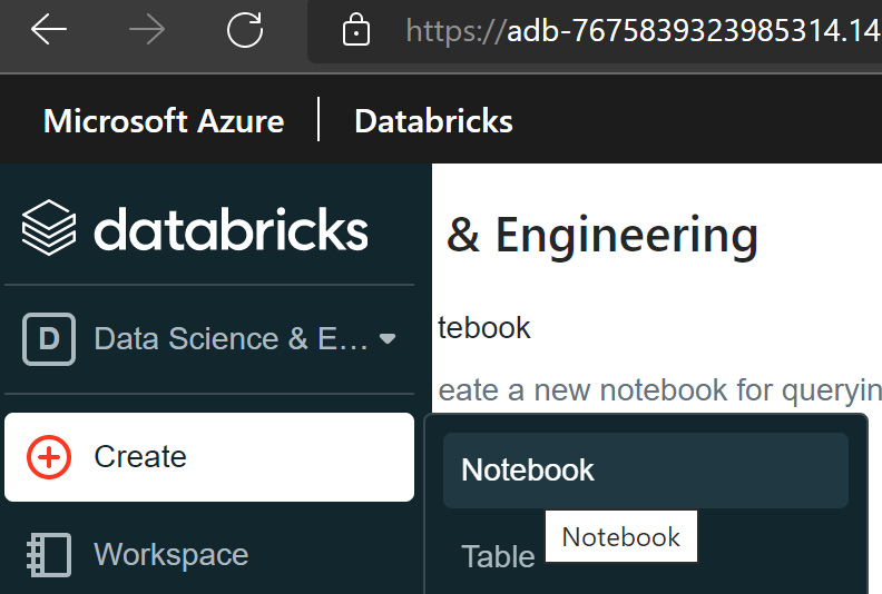
Figure 7.31 – Creating a notebook

3. Set the notebook name as processdata and Default Language to Scala:

Figure 7.32 – Creating the processdata notebook

4. In the File menu, click Upload Data:

Figure 7.33 – Uploading data

5. Click Drop files to upload, or click to browse. Make sure to also note down the default path in your environment. Usually, it will follow the following format – /FileStore/shared_uploads/<loginname>:

Figure 7.34 – Uploading data

6. Upload the covid-data.csv file downloaded at the beginning of this recipe:

Figure 7.35 – Uploading the covid-data.csv file

7. Execute the following command to read the data to a DataFrame. Ensure to replace the file path noted in step 6. Notice from the output message that the DataFrame contains over 60 fields:

   val covid_raw_data = spark.read.format("csv")

   .option("header", "true")

   .option("inferSchema", "true")

   .load("/FileStore/shared_uploads/[email protected]/covid_data.csv")

The result of the command is provided here:

Figure 7.36 – Reading the CSV data

8. At the right-hand corner of the cell, click on the drop-down button, and click Add Cell Below. Provide the following command to display the DataFrame:

   display(covid_raw_data)

The result of the command is provided here:

Figure 7.37 – Displaying the CSV data

9. Execute the following command to get the row count in the CSV file or DataFrame. There are over 94,000 rows:

   covid_raw_data.count()

The result of the command is provided here:

Figure 7.38 – Displaying the row count

10. Let’s remove any duplicates. The dropDuplicates() function removes duplicates and stores the result in a new DataFrame:

    val covid_remove_duplicates = covid_raw_data.dropDuplicates()

The result of the command is provided here:

Figure 7.39 – Removing duplicates

11. Let’s look at the fields and their data type in the DataFrame. The printSchema() function provides the DataFrame structure:

    covid_remove_duplicates.printSchema()

The result of the preceding command is provided in the following screenshot:

Figure 7.40 – Removing duplicates

12. The data is about the impact of COVID across the globe. Let’s focus on a handful of columns that are required, instead of all the columns provided. The select function can help us to specify the columns that we need out of a DataFrame. Execute the following command to load the selected columns to another DataFrame:

    val covid_selected_columns = covid_remove_duplicates.select("iso_code","location","continent","date","new_deaths_per_million","people_fully_vaccinated","population")

The result of the preceding command is provided in the following screenshot:

Figure 7.41 – Loading selected columns

13. For our analysis, let’s remove any rows that contain NULL values in any of the columns. The na.drop() function can help to achieve this. Execute the following command. The covid_clean_data DataFrame will only contain rows without any NULL value in them once the command has been executed. The covid_clean_data.count() command shows that only 32,000+ rows were without any NULL values:

    val covid_clean_data = covid_selected_columns.na.drop()

    covid_clean_data.count()

The result of the preceding command is provided in the following screenshot:

Figure 7.42 – Removing NULL values

14. Data analysis is easier to perform using Spark SQL commands. To use SQL commands to analyze a DataFrame, we need to create a temporary view. The following command will create a temporary view called covid_view:

    covid_clean_data.createOrReplaceTempView("covid_view")

The result of the preceding command is provided in the following screenshot:

Figure 7.43 – Creating a temporary view

15. Execute the following command to get some insights out of the data. %sql, on the first line, lets us switch from Scala to SQL. The SQL query provides the number of deaths, and the percentage of people vaccinated in each country with a population of over 1 million, ordered by countries with the highest deaths per million people:

    %sql

    SELECT iso_code, location, continent,

    SUM(new_deaths_per_million) as death_sum,

    MAX(people_fully_vaccinated * 100 / population) as percentage_vaccinated FROM covid_view

    WHERE population > 1000000

    GROUP BY iso_code,location,continent

    ORDER BY death_sum desc

The result of the command is provided here:

Figure 7.44 – Insights using the SQL query

16. To visualize the output from the previous SQL query, click on the chart icon and select Bar:

Figure 7.45 – Generating a bar graph

17. Click on Plot Options…:

Figure 7.46 – Plot options

18. Set Plot Options… as follows. Set location in the Keys section, continent in the Series groupings section, and death_sum in the Values section, as shown in the following screenshot. This will provide a bar graph with a line for each country, with the color of the line based on the continent that the country belongs to:

Figure 7.47 – Customizing the plot

19. You will get the following output. High spikes with green lines indicate that European countries were heavily affected by COVID:

Figure 7.48 – Visual insights

How it works…

DataFrames are the fundamental objects used to store runtime data during data processing in Databricks. DataFrames are in-memory objects and extremely well-optimized for performing advanced analytics operations.

A CSV file was loaded to the Databricks File System (DBFS) storage, which is the default local storage available when a Databricks workspace is created. We can perform the same activities in a data lake account too, by uploading the CSV file to the data lake container and mounting the data lake container, as explained in the Mounting an Azure Data Lake container in Databricks recipe.

After loading the data to a DataFrame, we were able to cleanse the data by performing operations such as removing unwanted columns, dropping duplicates, and deleting rows with NULL values easily using Spark functions. Finally, by creating a temporary view out of the DataFrame, we were able to analyze the DataFrame’s data using SQL queries and get visual insights using Databricks' visualization capabilities.

Scheduling notebooks using job clusters

Data processing can be performed using notebooks, but to operationalize it, we need to execute it at a specific scheduled time, depending upon the demands of the use case or problem statement. After a notebook has been created, you can schedule a notebook to be executed at a preferred frequency using job clusters. This recipe will demonstrate how you could schedule a notebook using job clusters.

Getting ready

Create a Databricks workspace, as explained in the Configuring the Azure Databricks environment recipe.

How to do it…

In the following steps, we will import the SampleJob.dbc notebook file into the Databricks workspace and schedule it to be run daily:

1. Log in to portal.azure.com. Go to All resources and find pactadedatabricks, the Databricks workspace created in the Configuring the Azure Databricks environment recipe. Click Launch Workspace to log in to the Databricks portal.
2. Navigate to Workspace | Create | Folder, as shown in the following screenshot:

Figure 7.49 – Creating folder insights

3. Create a folder called Job:

Figure 7.50 – Create a Job folder

4. Click Workspace, click on the Job folder, and pick the Import option:

Figure 7.51 – Importing a notebook

5. Pick the URL option to import the notebook. Paste the https://github.com/PacktPublishing/Azure-Data-Engineering-Cookbook-2nd-edition/blob/main/chapter07/SampleJob.dbc path to import a notebook called SampleJob:

Figure 7.52 – Importing a notebook

6. In the Job folder, you will have a notebook called SampleJob. The SampleJob notebook will read a sample CSV file and provide insights from it:

Figure 7.53 – The imported notebook

7. From the menu on the left, click Jobs:

Figure 7.54 – Jobs in the Create menu

8. Click Create Job:

Figure 7.55 – Create Job

9. Provide a job name of SampleJob. Select the imported SampleJob notebook. On the New Cluster configuration, click on the edit icon to set the configuration options. The job will create a cluster each time it runs based on the configuration and delete the cluster once the job is completed:

Figure 7.56 – Editing the cluster configuration

10. Reduce the total number of cores to 2 and hit the Confirm button to save the cluster configuration. Hit the Create button on the job creation screen:

Figure 7.57 – Save the cluster configuration

11. Hit the Edit schedule button to edit the schedule:

Figure 7.58 – Edit schedule configuration

12. Set Schedule Type to Scheduled and set a frequency as per your needs. Hit the Save button:

Figure 7.59 – Setting the schedule configuration

13. Hit Run now to trigger the job:

Figure 7.60 – Run now

14. Click on Runs on the left tab to view the job run result:

Figure 7.61 – Job runs

15. The Active runs section will provide the currently active jobs. After a few minutes, the job will move to the Running state from the initial Pending state:

Figure 7.62 – Job runs

16. Upon completion, the job result will be listed as completed in the Completed runs (past 60 days) section. Click Start time to view the result of the completed notebook:

Figure 7.63 – A completed run

17. The job execution result is shown in the following screenshot:

Figure 7.64 – The notebook output

18. If we need to execute another notebook at the same schedule, we could create an additional task within the same job. Go back to the job menu and click on SampleJob. Switch to the Tasks section. Click on the + button to add a new task:

Figure 7.65 – Adding a new task

19. Provide a task name. You may add any notebook to the task. Notice that the cluster name is SampleJob_cluster, which implies that it will use the cluster created for the previous task. The Depends on option controls whether the job needs to run after the previous SampleJob task is completed:

Figure 7.66 – Adding a new task

20. Upon adding it, the two tasks will appear, as shown here:

Figure 7.67 – Multiple tasks

How it works…

The imported notebook was set to run at a specific schedule using the Databricks job scheduling capabilities. While scheduling the jobs, New Cluster was selected, instead of picking any cluster available in the workspace. Picking New Cluster implies a cluster will be created each time the job runs and will be destroyed once the job completes. This also means the jobs need to wait for an additional 2 minutes for the cluster to be created for each run.

Adding multiple notebooks to the same job via additional tasks allows us to reuse the job cluster created for the first notebook execution, and the second task needn’t wait for another cluster to be created. Usage of multiple tasks and the dependency option allows us to orchestrate complex data processing flows using Databricks notebooks.

Working with Delta Lake tables

Delta Lake databases are Atomicity, Consistency, Isolation, and Durability (ACID) property-compliant databases available in Databricks. Delta Lake tables are tables in Delta Lake databases that use Parquet files to store data and are highly optimized for performing analytic operations. Delta Lake tables can be used in a data processing notebook for storing preprocessed or processed data. The data stored in Delta Lake tables can be easily consumed in visualization tools such as Power BI.

In this recipe, we will create a Delta Lake database and Delta Lake table, load data from a CSV file, and perform additional operations such as UPDATE, DELETE, and MERGE on the table.

Getting ready

Create a Databricks workspace and a cluster, as explained in the Configuring the Azure Databricks environment recipe of this chapter.

Download the covid-data.csv file from this link: https://github.com/PacktPublishing/Azure-Data-Engineering-Cookbook-2nd-edition/blob/main/chapter07/covid-data.csv.

Upload the covid-data.csv file to the workspace, as explained in step 1 to step 6 of the How to do it… section of the Processing data using notebooks recipe.

How to do it…

In this recipe, let’s create a Delta Lake database and tables, and process data using the following steps:

1. From the Databricks menu, click Create and create a new notebook:

Figure 7.68 – A new notebook

2. Create a notebook called Covid-DeltaTables with Default Language set to SQL:

Figure 7.69 – Delta notebook creation

3. Add a cell to the notebook and execute the following command to create a Delta database called covid:

   CREATE DATABASE covid

The output is displayed in the following screenshot:

Figure 7.70 – Delta database creation

4. Execute the following command to read the covid-data.csv file to a temporary view. Please note that the path depends on the location where covid-data.csv was uploaded and ensure to provide the correct path for your environment:

   CREATE TEMPORARY VIEW covid_data

   USING CSV

   OPTIONS (path "/FileStore/shared_uploads/[email protected]/covid_data.csv", header "true", mode "FAILFAST")

The output is displayed in the following screenshot:

Figure 7.71 – Temporary view creation

5. Execute the following command to create a Delta table using the temporary view. USING DELTA in the CREATE TABLE command indicates that it’s a Delta table being created. The location specifies where the table is stored. If you have mounted a data lake container (as we did in the Mounting an Azure Data Lake container in Databricks recipe), you can use the data lake mount point to store the Delta Lake table in your Azure Data Lake account. In this example, we use the default storage provided by Databricks, which comes with each Databricks workspace.

The table name is provided in <database name>.<table name> to ensure it belongs to the Delta Lake database created. To insert the data from the view into the new table, the table is created using the CREATE TABLE command, followed by the AS command, followed by the SELECT statement against the view:

CREATE OR REPLACE TABLE covid.covid_data_delta

USING DELTA

LOCATION ‘/FileStore/shared_uploads/[email protected]/covid_data_delta’

AS

SELECT iso_code,location,continent,date,new_deaths_per_million,people_fully_vaccinated,population FROM covid_data

The output is displayed in the following screenshot:

Figure 7.72 – Creating the Delta table

6. Go to the Databricks menu, click Data, and then click on the covid database. You will notice that a covid_data_delta table has been created:

Figure 7.73 – The created Delta table

7. Go back to the notebook we were working on. Add a new cell and delete some rows using the following command. The DELETE command will delete around 57,000 rows. We can delete, select, and insert data as well as we would in any other commercial database:

   DELETE FROM covid.covid_data_delta where population is null or people_fully_vaccinated is null or new_deaths_per_million is null or location is null

The output is displayed in the following screenshot:

Figure 7.74 – Deleting a few rows in a Delta table

8. Add a new cell and execute the following command to delete all the rows from the table. Let’s run a select count(*) query against the table, which will return 0 if all the rows have been deleted:

   delete from covid.covid_data_delta;

   Select count(*) from covid.covid_data_delta;

The output is displayed in the following screenshot:

Figure 7.75 – Deleting all rows

9. Delta tables have the ability to time travel, which allows us to read older versions of the table. Using the as of version <version number> keyword, we can read the older version of the table. Version 0 gives the most recent version behind the current version of the table. Add a new cell and execute the following command to read the data before deletion:

   select * from covid.covid_data_delta version as of 0;

The output is displayed in the following screenshot:

Figure 7.76 – Check out an older version of the Delta table

10. RESTORE TABLE can restore the table to the older version. Add a cell and execute the following command to recover all the rows before deletion:

    RESTORE TABLE covid_data_delta TO VERSION AS OF 0

The output is displayed in the following screenshot:

Figure 7.77 – Restoring the table to an older version

11. Let’s perform an UPDATE statement, followed by a DELETE statement. Add two cells. Paste the following commands into these cells, as shown in the following screenshot. Execute them in sequence:

    UPDATE covid_data_delta SET population = population * 1.2 WHERE continent = ‘Asia’;

    DELETE FROM covid_data_delta  WHERE continent = ‘Europe’;

The output is displayed in the following screenshot:

Figure 7.78 – Update and delete

12. If we want to revert these two operations (UPDATE and DELETE), we can use the MERGE statement and the Delta table’s row versioning capabilities to achieve this. Using a single MERGE statement, we can perform the following:
    • Compare the older version of the table with the current version of the table
    • If the rows match, update all the columns with values from the older version
    • If the row doesn’t match, insert the row from the older version into the current table

This can be achieved using the following code:

MERGE INTO covid_data_delta source

  USING covid_data_delta TIMESTAMP AS OF "2022-02-19 16:45:00" target

  ON source.location = target.location and source.date = target.date

  WHEN MATCHED THEN UPDATE SET *

  WHEN NOT MATCHED

  THEN INSERT *

The MERGE command takes the covid_data_delta table as the source table to be updated or inserted. Instead of specifying version numbers, we can also use timestamps to obtain older versions of the table. covid_data_delta TIMESTAMP AS OF "2022-02-19 16:45:00" takes the version of the table as of February 19, 2022, 16:45:00 – UTC time. WHEN MATCHED THEN UPDATE SET * updates all the columns in the table when the condition specified in the ON clause matches. When the condition doesn’t match, the rows are inserted from the older version to the current version of the table. The output, as expected, shows that the rows that were deleted in step 11 were successfully reinserted:

Figure 7.79 – The merge statement

How it works…

Delta tables offer advanced capabilities for processing data, such as support for UPDATE, DELETE, and MERGE statements. MERGE statements and the versioning capabilities of Delta tables are very powerful in ETL scenarios, where we need to perform UPSERT (update if it matches, insert if it doesn’t) operations against various tables.

These capabilities for supporting data modifications and row versioning are made possible because Delta tables maintain the changes to the table via a transaction log file stored in JSON format. The transaction files are located in the same location where the table was created but in a subfolder called _delta_log. By default, the log files are retained for 30 days and can be controlled using the delta.logRetentionDuration table property. The ability to read older versions is also controlled by the delta.logRetentionDuration property.

Connecting a Databricks Delta Lake table to Power BI

Delta Lake databases are commonly used to store processed data in Delta Lake tables, which is then ready to be consumed by reporting-layer applications such as Power BI. Delta Lake tables are best suited for handling analytic workloads from Power BI, as Delta Lake tables use Parquet files as storage, which offer optimal performance for analytic workloads.

In this recipe, we will use Power BI Desktop, connect to a Delta Lake table, and build a simple report in Power BI.

Getting ready

Create a Databricks workspace and a cluster as explained in the Configuring the Azure Databricks environment recipe.

Download the latest version of Power BI Desktop from https://powerbi.microsoft.com/en-us/downloads/ and install Power BI Desktop on your machine.

How to do it…

Perform the following steps to connect a Delta Lake table to a Power BI report and create visualizations:

1. Log in to the Databricks portal and click on the Compute button in the menu:

Figure 7.80 – Compute

2. Click on the cluster and start it if the cluster is terminated. Click on Advanced options:
   

Figure 7.81 – Advanced options for the cluster

3. Click on the JDBC/ODBC section. Copy the values from the Server Hostname and HTTP Path sections. We will need them when connecting to the Delta Lake table using Power BI Desktop:

Figure 7.82 – The JDBC/ODBC connection string

4. Click on the Workspace button in the Databricks menu. Click on any folder (by default under your username) and click on the Import button:

Figure 7.83 – Importing the notebook

5. For the Import from option, pick URL. Provide https://github.com/PacktPublishing/Azure-Data-Engineering-Cookbook-2nd-edition/blob/main/chapter07/Delta_PowerBI.dbc as the input and click the Import button:

Figure 7.84 – Import notebook

6. This notebook will read a CSV file, create a database called PowerBI, and create a Delta table called Diamond_Insights_PowerBI. Click on the Run All button in the top-right corner of the notebook:

Figure 7.85 – Run all cells

7. Open the installed Power BI Desktop:

Figure 7.86 – Start Power BI Desktop

8. Click Get data and then More…:

Figure 7.87 – Starting Power BI Desktop

9. Select Azure Databricks and click on the Connect button:

Figure 7.88 – Connecting to Databricks

10. Provide the Server Hostname value and the HTTP Path value noted in step 3, and click on the Ok button:

Figure 7.89 – Connecting to the Delta database

11. Sign in to Azure using the Azure account that you used to create the Databricks workspace:

Figure 7.90 – Connecting to Azure

12. Once you're signed in, press the Connect button:

Figure 7.91 – Connecting to the Delta table

13. Expand hive_metastore and then the powerbi database. Select the diamond_insights_powerbi table and click on the Load button:

Figure 7.92 – Loading the Delta table

14. Select the color and price columns on the right-hand side. Set the Visualizations type to Clustered column chart. This will show the price of diamonds by color code. This will indicate that color code G has the highest price:

Figure 7.93 – Adding a clustered column chart

15. Click on the white space anywhere outside of the clustered column chart visual. Click on the cut and price columns and set the Visualizations type to Clustered column chart. Now, you will have added another visual:

Figure 7.94 – Adding another visual

16. Click on the bar against the Ideal value on the price by cut visual. The price by color visual will be automatically filtered and will show that color G contributes close to 20 million in price when the cut is Ideal:

Figure 7.95 – Get insights using visuals

17. Open the File menu and hit the Save button to save the Power BI report.

How it works…

We used the Azure AD credentials to sign in to Azure Databricks and extracted the connection string from the Databricks cluster. When the connection request comes from Power BI, Databricks authenticates using Azure AD credentials. For the authentication to succeed, the Databricks cluster needs to be up and running. Once authenticated, Delta Lake tables are accessible, just as with any other database tables using Power BI. We added two simple visuals to explore the data visually. Clicking on one of the visuals automatically filters the other visual, which allows us to get insights out of the data easily.