8

Processing Data Using Azure Synapse Analytics

Azure Synapse Analytics workspaces generation 2, formally released in December 2020, is the industry-leading big data solution for processing and consolidating data of business value. Azure Synapse Analytics has three important components:

• SQL pools and Spark pools for performing data exploration and processing
• Integration pipelines for performing data ingestion and data transformations
• Power BI integration for data visualization

Having data ingestion, processing, and visualization capabilities in a single service with seamless integration with all other services makes Azure Synapse Analytics a very powerful tool in big data engineering projects. This chapter will introduce you to Synapse workspaces and cover the following recipes:

• Provisioning an Azure Synapse Analytics workspace
• Analyzing data using serverless SQL pool
• Provisioning and configuring Spark pools
• Processing data using Spark pools and a lake database
• Querying the data in a lake database from serverless SQL pool
• Scheduling notebooks to process data incrementally
• Visualizing data using Power BI by connecting to serverless SQL pool

By the end of the chapter, you will have learned how to provision a Synapse workspace and Spark pools, explore and analyze data using serverless SQL pool and Spark pools, create a lake database and query a lake database from serverless SQL pool and a Spark pool, and finally, visualize the lake database data in Power BI.

Technical requirements

For this chapter, you will need the following:

• A Microsoft Azure subscription
• PowerShell 7
• Power BI Desktop

Provisioning an Azure Synapse Analytics workspace

In this recipe, we’ll learn how to provision a Synapse Analytics workspace. A Synapse Analytics workspace is the logical container that will hold the Spark pools, SQL pool, and integration pipelines that are required for the data engineering tasks.

Getting ready

To get started, log into https://portal.azure.com using your Azure credentials.

How to do it…

Follow these steps to create a Synapse Analytics workspace:

1. Go to the Azure portal home page at portal.azure.com and click on Create a resource. Search for Synapse and select Azure Synapse Analytics. Click the Create button:

Figure 8.1 – Creating a Synapse Analytics workspace

2. Provide the following details:
   1. Create a new resource group called PacktADESynapse by clicking the Create new link.
   2. Provide a unique workspace name. For this example, we are using packtadesynapse. You may pick any location.
   3. Provisioning a Synapse Analytics workspace requires an Azure Data Lake Storage Gen2 account. You may use an existing account or create a new account using the Create new link. Let’s create a new Azure Data Lake Storage Gen2 account called packatadesynapse by clicking the Create new link.
   4. A Synapse Analytics workspace requires a container on the new data lake account provisioned. Let’s create a new container named synapse by clicking the Create new link. After the Synapse workspace is provisioned, the Synapse workspace service account is given permissions on the data lake account and the container by default. We will be able to connect to the data stored in the storage account from the Synapse workspace seamlessly. The data lake account will be used to store a lake database (a component of Synapse Spark pools) and other artifacts of the Synapse workspace. Click the Next: Security > button at the bottom:

Figure 8.2 – Setting up Project details in a Synapse Analytics workspace

5. On occasion, Azure subscriptions may not be able to create a Synapse workspace because of a Resource provider not registered for the subscription error. To resolve the error, go to the Azure portal and open your subscription. Click the Resource providers section, search for the Synapse resource, and register Microsoft.Synapse on the subscription. Please refer to https://docs.microsoft.com/en-us/azure/azure-resource-manager/management/resource-providers-and-types#azure-portal for detailed steps on how to register a resource on a subscription.

3. On the Security page, we will be filling in the user ID and password details for SQL pool. Provide the user ID and password as sqladminuser and PacktAdeSynapse123. Click Review + Create to create the Synapse Analytics workspace:

Figure 8.3 – Creating SQL pool in a Synapse Analytics workspace

The preceding steps will create a Synapse Analytic workspace and a storage account. In the subsequent recipes of this chapter, we will use the workspace to explore and process data using SQL pool and Spark pool.

Analyzing data using serverless SQL pool

Serverless SQL pool allows us to explore data using T-SQL commands in a Synapse Analytics workspace. The key advantage of serverless SQL pool is that it is available by default once a Synapse Analytics workspace is provisioned with no cluster or additional resources to be created. In serverless SQL pool, you will be charged only for the data processed by the queries as it is designed as a pure pay-per-use model.

Getting ready

Create a Synapse Analytics workspace, as explained in the Provisioning an Azure Synapse Analytics workspace recipe of this chapter.

How to do it…

In this recipe, we will perform the following:

• Uploading sample data into a Synapse Analytics workspace data lake account and querying it using serverless SQL pool
• Creating a serverless SQL database and defining a view to read the data stored in the data lake account

The detailed steps to perform these tasks are as follows:

1. Log in to portal.azure.com, go to All resources, and search for packtadesynapse, the Synapse Analytics workspace we created in the Provisioning an Azure Synapse Analytics workspace recipe. Click the workspace. Click Open Synapse Studio:

Figure 8.4 – Open Synapse Studio

2. Click on the blue cylinder (the data symbol) on the left, which will take you to the Data section. Click the Linked tab. Expand the data lake account of the Synapse workspace (packtadesynapse for this example) and click on the synapse (Primary) container. Click the + New folder button and create a folder called CSV:

Figure 8.5 – Synapse studio folder creation

3. Download the covid-data.csv file from https://github.com/PacktPublishing/Azure-Data-Engineering-Cookbook-2nd-edition/blob/main/chapter07/covid-data.csv to your local machine.
4. Double click on the CSV folder in Synapse Studio. Click on the Upload button and upload the covid-data.csv file from your local machine into the data lake account of the Synapse workspace:

Figure 8.6 – Synapse Studio folder creation

5. After the file has uploaded, right-click the covid-data.csv file in the CSV folder, select New SQL script, and click the Select TOP 100 rows option:

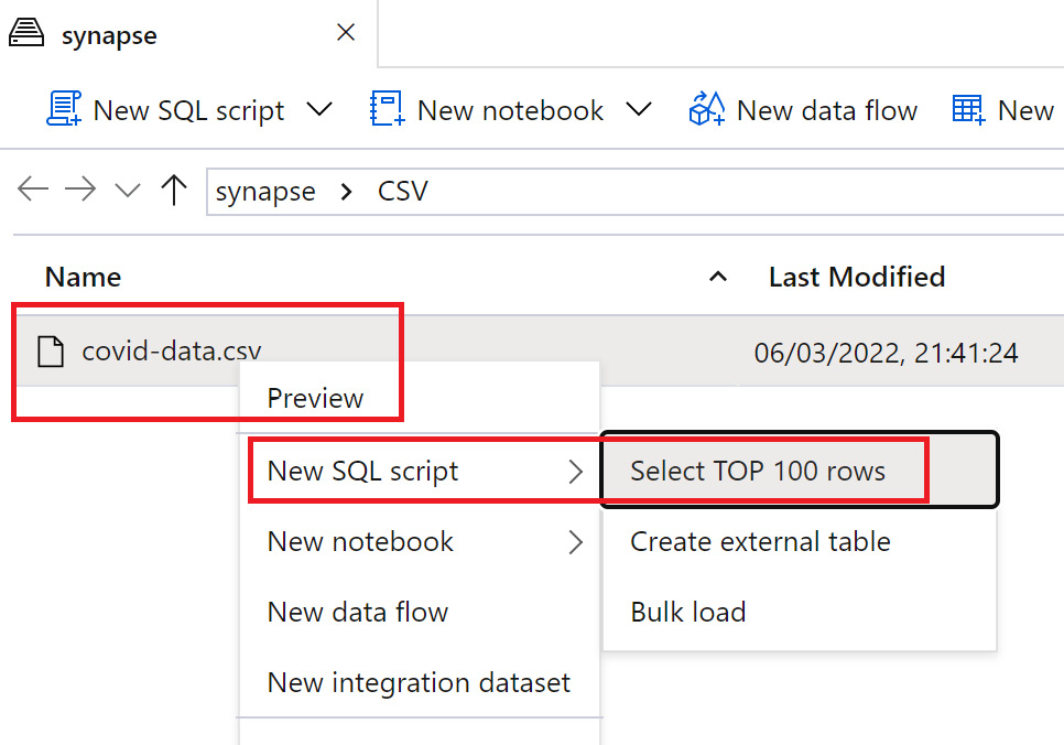
Figure 8.7 – Synapse Studio folder creation

6. A new query window will open with a script using the OPENROWSET command. Click the Run button to execute the query and preview the data:

Figure 8.8 – Querying data using OPENROWSET

7. Let’s perform the following. Let’s create a serverless database and a view referencing the OPENROWSET command to read the covid-data.csv file. We notice that the actual column names (iso_code, continent, location, and date) are listed in the first row. These columns (iso_code, continent, location, and date) need to move up to become the table’s column names and we need to remove the existing column names (C1, C2, C3, C4, and so on). We can fix that by adding the HEADER_ROW = TRUE option after the PARSER_VERSION option in the OPENROWSET command. Use the following command to create a database, create a view, and fix the header:

   CREATE DATABASE serverless

   GO

   USE serverless

   GO

   CREATE VIEW covid AS

   SELECT

      *

   FROM

       OPENROWSET(

           BULK 'https://packatadesynapse.dfs.core.windows.net/synapse/CSV/covid-data.csv',

           FORMAT = 'CSV',

     PARSER_VERSION = '2.0'

   , HEADER_ROW = TRUE

       ) AS [result]

The result of the query execution is demonstrated here:

Figure 8.9 – Create view in serverless SQL

8. Click on the icon that looks like a notebook on the left-hand side of the screen. This will take you to the Develop section. Click the + button on top and click SQL script:

Figure 8.10 – A new SQL script

9. Use the following script, referencing the serverless database and the view created, to find a list of countries that have the maximum number of deaths per million people on a given day:

   use serverless

   GO

   Select iso_code,location , continent,

   max(isnull(new_deaths_per_million,0)) as death_sum,

   max(isnull(people_fully_vaccinated,0) / isnull(population,0)) * 100 as percentage_vaccinated From covid

   where isnull(population,0) > 1000000

   group by iso_code,location,continent

   order by death_sum desc

The output of the preceding query is shown in the following screenshot:

Figure 8.11 – Querying the serverless view

How it works…

After we uploaded the covid-data.csv file to the Azure Data Lake Storage account associated with the Synapse workspace, we were able to query the data at the click of a button, without providing any credentials or provisioning any other resources. Serverless SQL pool, which is available by default in a Synapse workspace, allows us to interact with the data with minimal effort.

We used the OPENROWSET function to read the data from a CSV file and we encapsulated it inside a view for easier access in subsequent scripts. The serverless database and the view can also be accessed from other services such as Power BI and Data Factory. Serverless SQL pool, with its ability to define views, can be used to create a logical data warehouse on top of a data lake storage account, which will serve as a powerful tool for data analysis and exploration.

Provisioning and configuring Spark pools

A Spark pool is an important component of Azure Synapse Analytics that allows us to perform data exploration and processing using the Apache Spark engine. Spark pools in Azure Synapse Analytics allow us to process data using programming languages such as PySpark, Scala, C#, and Spark SQL. In this recipe, we will learn how to provision and configure Spark pools in Synapse Analytics.

Getting ready

Create a Synapse Analytics workspace, as explained in the Provisioning an Azure Synapse Analytics workspace recipe.

How to do it…

Let’s perform the following steps to provision a Spark pool in an Azure Synapse Analytics workspace:

1. Log in to portal.azure.com and click All Resources. Search for packtadesynapse, the Synapse Analytics workspace created in the Provisioning an Azure Synapse Analytics workspace recipe. Click on the workspace. Search for Apache Spark pools under Analytics pools. Click + New:

Figure 8.12 – Creating Spark pools

2. Fill in the details as follows:
   1. Name the Spark pool packtsparkpool.
   2. The Node size family property indicates the type of virtual machines that will be running to process the big data workload. Let’s pick Memory Optimized, as it’s typically good enough for general purpose data processing tasks. The Hardware accelerated type provides GPU-powered machines meant for performing heavy-duty data science and big data workloads.
   3. The Node size property indicates the compute and memory of virtual machines in a Spark pool. Let’s pick Small (4 vCores / 32 GB), as it’s the cheapest option.
   4. Autoscale allows the Spark pool to allocate additional nodes or machines depending upon the workload. Let’s leave it as Enabled.
   5. Set the minimum and maximum Number of nodes to 3 and 10. A Spark pool can autoscale up to a maximum of 10 machines/nodes. Click on Next: Additional settings >:

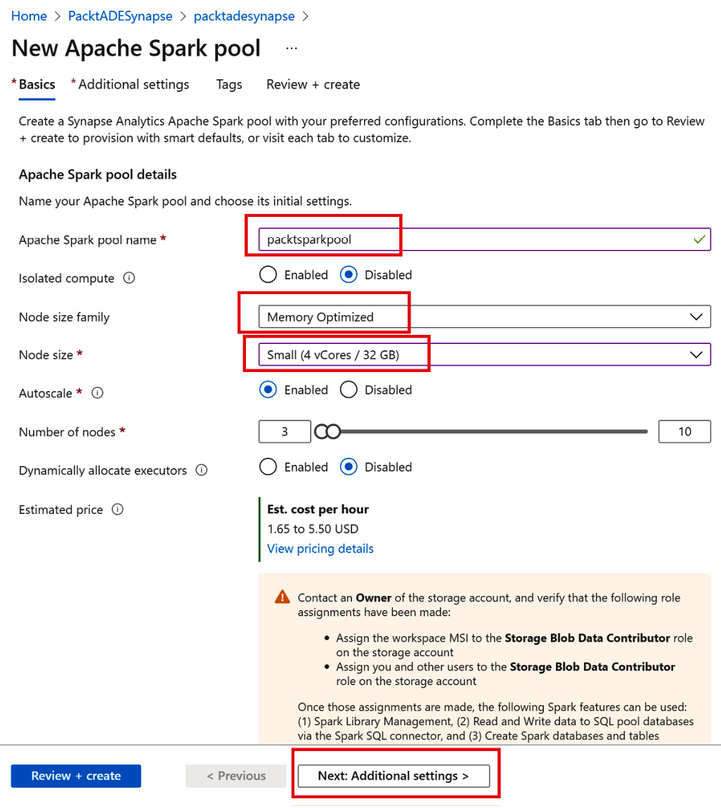
Figure 8.13 – Creating Spark pools

6. Leave Automatic pausing as Enabled. Automatic pausing stops the Spark pool when there are no jobs being processed.
7. Set Number of minutes idle to 10. This ensures that the pool is paused if no job is running for 10 minutes.
8. Set the Apache Spark version to the latest one (3.1 here, as of March 2022), as it ensures that we get the latest Java, Scala, .NET, and Delta Lake versions. Click Review + create:

Figure 8.14 – Configuring Spark pools

How it works…

Creating a Spark pool defines the configuration for the nodes/virtual machines, which will be processing the big data workload as it arrives. Each time a new user logs in and submits a Spark job/Spark notebook to process data, an instance of Spark pool is created. An instance of Spark pool is basically a bunch of virtual machines/nodes configured as defined in the Spark pool configuration. A single user can use up to the maximum number of nodes defined in the pool. If there are multiple users connecting to the Spark pool, Synapse will create as many instances of Spark pool as the number of users. You will be billed for the number of active instances and for the time period during which they were active. Billing will stop for a particular instance if it remains idle longer than the idle time period defined in the Spark pool configuration.

Processing data using Spark pools and a lake database

Spark pools in a Synapse workspace allow us to process data and store them as tables inside a lake database. A lake database allows us to create tables using CSV files, Parquet files, or as Delta tables stored in the data lake account. Delta tables use Parquet files for storage and support insert, update, delete, and merge operations. Delta tables are stored in a columnar format, which is compressed, ideal for storing processed data and supporting analytic workloads. In this recipe, we will read a CSV file, perform basic processing, and load the data into a Delta table in a lake database.

Getting ready

Create a Synapse Analytics workspace, as explained in the Provisioning an Azure Synapse Analytics workspace recipe.

Create a Spark pool cluster, as explained in the Provisioning and configuring Spark pools recipe.

We need to upload the covid-data.csv file from https://github.com/PacktPublishing/Azure-Data-Engineering-Cookbook-2nd-edition/blob/main/chapter07/covid-data.csv to a folder named CSV in the data lake account attached to the Synapse Analytics workspace. To do so, follow step 1 to step 4 in the How to do it… section from the Analyzing data using serverless SQL pool recipe.

How to do it…

After uploading the covid-data.csv file to the CSV folder in the data lake account, let’s perform the following steps to process the data in the CSV file and load it into a Delta Lake table in a lake database:

1. Log in to portal.azure.com, click All resources, search for packtadesynapse, the Synapse Analytics workspace we created, and click on it. Click Open Synapse Studio.
2. Click on the data icon on the left, click the Linked tab, and expand the Azure Data Lake Storage Gen2 | packtadesynapse | synapse (Primary) container. Navigate to the CSV folder inside the synapse container, where the covid-data.csv file has been uploaded. Right-click on the covid-data.csv file, select the option New notebook | Load to DataFrame:

Figure  8.15 – Load to DataFrame

3. A new notebook will be created. Notebooks are used by data engineers to develop the code that will be used to process data using Synapse pools. Attach the notebook to packtsparkpool, the Synapse Spark pool created in the Provisioning and configuring Spark pools recipe in this chapter, using the Attach to drop-down menu at the top of the notebook. Uncomment the fourth line in the first cell by removing ##, as our file contains a header. Hit Run Cell (which looks like a play button) on the left:

Figure  8.16 – The data loaded to the DataFrame

4. Data will be loaded to a DataFrame called df using the automatic PySpark code generated. Let’s use the Spark SQL language to understand the data. To interact with the data using Spark SQL, we need to create a temporary view. The createOrReplaceTempView command helps to create a temporary view that will be visible only within the notebook. Add a new cell by hitting the + Code button, paste the following command, and run the new cell:

   df.createOrReplaceTempView("v1")

The output is displayed in the following screenshot:

Figure 8.17 – Creating a temporary view

5. To check out which columns are present in the covid-data.csv file, let’s use the Describe Spark SQL command to list the columns in the view. Add a new cell and paste the following command. The %%sql command switches the programming language from PySpark to Spark SQL. We will notice that the view contains several columns (use the scroll bar to check out all of them). All the columns are also of the string data type:

   %%sql

   Describe v1;

The output is as follows:

Figure 8.18 – The list columns

6. Let’s focus on the following key columns – date, continent, location, new_cases, and new_deaths. Let’s also change the data type of new_cases and new_deaths to integer and load it into a Delta table. To load it into a Delta table, we need to create a lake database first, create the new Delta table, and then load the data. The Create database command creates the database, and Create table <tablename> using Delta as <Select statement> creates the table and loads the data. Copy the following command to a new cell and run the new cell:

   %%sql

   Create database sparksqldb;

   Create or replace table sparksqldb.covid

   USING Delta

   AS

   Select date, continent,location, CAST(new_cases as int) as new_cases,

   CAST(new_deaths as int) as new_deaths from v1

The output of the preceding query is as follows:

Figure  8.19 – Creating a Delta table

7. In the previous step, we created a lake database called sparksqldb and a Delta table inside it called covid. Using the delta option in the CREATE or REPLACE TABLE command ensured that the table was created as a Delta table. The CAST function in the SELECT statement changed the column data type to INTEGER. Verify the data-type change using the DESCRIBE command:

   %%sql

   Describe table sparksqldb.covid;

The result of the query execution is demonstrated in the following screenshot:

Figure 8.20 – The Delta table structure

8. Let’s delete the rows that have NULL values in the continent column. Add a new cell and copy-paste the following command:

   %%sql

   Delete from sparksqldb.covid where continent is NULL

The output of the preceding query is as follows:

Figure  8.21 – Using a Delete statement on a Delta table

9. Delta tables have a feature called time travel, which lets us explore the previous versions of the table. We will use time travel to query the deleted rows (rows with NULL values in the continent column). To perform that as a first step, we need to find the location where the Delta table is stored. The Describe detail command will provide a column called location, which will contain the location of the Delta table. Add a new cell, copy the following command, and run the cell. Copy the contents of the location column. Ensure to expand the column by dragging the slider to your right and copying the full path of the Delta table:

   %%sql

   DESCRIBE DETAIL sparksqldb.covid  

The output of the preceding query is as follows:

Figure 8.22 – Get the Delta table location

10. On the copied location, remove the text that starts with abfss and goes up to windows.net. We only need the path that starts from the container name (synapse), not the storage account or protocol details. For example, if your copied location is abfss://[email protected]/synapse/workspaces/packtadesynapse/warehouse/sparksqldb.db/covid, remove abfss://[email protected]/ and retain /synapse/workspaces/packtadesynapse/warehouse/sparksqldb.db/covid.
11. Add a new cell and copy the following Spark command. Paste the edited location path to the load function. The Option("versionAsOf",0) function makes the command read the older version of the table. The second parameter in the option function indicates the version number to be read. Version number 0 would be the most recent previous version of the table, version number 1 would be the next version older than version 0, and so on. The command reads the older data to a DataFrame, which we load to a view called old_Data:

    df2 =  spark.read.format("delta").option("versionAsOf", 0).load("/synapse/workspaces/packtadesynapse/warehouse/sparksqldb.db/covid")

    df2.createOrReplaceTempView("old_Data")

The result of the query execution is demonstrated in the following screenshot:

Figure 8.23 – Reading an old version of the Delta table

12. Execute a SELECT statement against the old_Data view to check out the rows that were deleted. Add a new cell, copy the following command, and execute the new cell. We will be able to read the deleted rows using the time travel feature on the Delta table:

    %%sql

    SELECT * FROM old_Data WHERE continent IS NULL

The result of the query execution is demonstrated in the following screenshot:

Figure  8.24 – SELECT statement on Delta table

How it works…

The Spark pools in a Synapse workspace allow us to seamlessly load CSV files to Delta tables using notebooks. Notebooks allow us to effortlessly switch between PySpark and SQL. Delta tables support data manipulation commands such as update, delete, and merge, and capabilities such as time travel make it very efficient for data processing tasks in data engineering projects.

Querying the data in a lake database from serverless SQL pool

Lake databases are created from Synapse Spark pools and typically consist of Delta tables. The following recipe will showcase how we could read the data stored in Delta tables from serverless SQL pool.

Getting ready

Create a Synapse Analytics workspace, as explained in the Provisioning an Azure Synapse Analytics workspace recipe in this chapter.

Create a Spark pool, as explained in the Provisioning and configuring Spark pools recipe in this chapter.

Create a lake database and Delta table, as explained in the Processing data using Spark pools and lake database recipe in this chapter.

How to do it…

Perform the following steps to query the data:

1. Log in to portal.azure.com, click All Resources, search for packtadesynapse, the Synapse Analytics workspace that we created, and click on it. Click Open Synapse Studio. Click on the data icon on the left, click the Linked tab, and expand the Azure Data Lake Storage Gen2 | packtadesynapse | synapse (Primary) container. Navigate to the following folder path: /synapse/workspaces/packtadesynapse/warehouse/sparksqldb.db. The usual path structure is <SynapseContainerName>/synapse/workspaces/<WorkspaceName>/warehouse/<lakedatabasename.db>. So, if you have named your lake database or table name differently, then it will vary from mine here. You will find a folder with the Delta table name (covid). Right-click on it and select New SQL script | Create external table:

Figure 8.25 – Create external table

2. Synapse will detect the file type and schema. Hit Continue to generate the external table creation script:

Figure 8.26 – Generation of the external table script

3. Leave the Select SQL pool option as Built-in. Built-in is the in-built serverless SQL pool. Select + New to create a new serverless database:

Figure 8.27 – A new serverless database

4. Name the database ServerlessSQLdb and click the Create button:

Figure 8.28 – Create a serverless database

5. Name the external table dbo.covid_ext. Click Open script:

Figure 8.29 – Creating an external table

6. To create an external table in Synapse SQL pool, we need to create the following objects: an external file format and an external data source first. Using Synapse Studio, we can generate the script to create the external file format, external data source, and external table. Select ServerlessSQLdb from the Use database dropdown and click the Run button to create the external table:

Figure 8.30 – Creation of the external table

7. Upon clicking the Run button, we will be able to see the data read from the external table successfully:

Figure 8.31 – Reading the external table

How it works…

To access the Delta table in a lake database, we need to create an external table in serverless SQL pool. We identified the folder where the Delta table was stored and we created an external table against it in serverless SQL pool. The external table acts as a link to the files stored in the Delta table. While the files reside in the Delta table, files appear as a table to end users in Serverless SQL pool. So, when a user queries the external table using a T-SQL script in serverless SQL pool, it will seamlessly read from the Delta table’s files and present it in a tabular format.

The lake database created a folder for each Delta table. So, it made it easier for us to create an external table against the folder of the Delta Lake table, which implies that we can seamlessly query the data from lake database Delta table in a serverless SQL pool database via external table. Changes to the Delta table are handled by adding or removing Parquet files inside the Delta Lake table folder using the Apache Spark engine. As we have created the external table against the table’s folder (not against any specific file), all the changes happening in the Delta Lake table will immediately be reflected in the serverless SQL pool’s external table without any additional effort.

Scheduling notebooks to process data incrementally

Consider the following scenario. Data is loaded daily into the data lake in the form of CSV files. The task is to create a scheduled batch job that processes the files loaded daily, performs basic checks, and loads the data into the Delta table in the lake database. This recipe addresses this scenario by covering the following tasks:

1. Only reading the new CSV files that are loaded to the data lake daily using Spark pools and notebooks
2. Processing and performing upserts (update if the row exists, insert if it doesn’t), and loading data into the Delta lake table using notebooks
3. Scheduling the notebook to operationalize the solution

Getting ready

Create a Synapse Analytics workspace, as explained in the Provisioning an Azure Synapse Analytics workspace recipe in this chapter.

Create a Spark pool, as explained in the Provisioning and configuring Spark pools recipe in this chapter.

Download the TransDtls-2022-03-20.csv file from https://github.com/PacktPublishing/Azure-Data-Engineering-Cookbook-2nd-edition/blob/main/chapter08/TransDtls-2022-03-20.csv. Create a folder called transaction-data inside the synapse container in the packtadesynapse data lake account. You can use Synapse Studio’s data pane to do the same. For detailed instructions on creating a folder and manually uploading files to Synapse Studio, refer to step 1 to step 4 in the How to do it… section of the Analyzing data using serverless SQL Pool recipe. Upload the file, as shown in the following picture:

Figure 8.32 – Uploading the file

How to do it…

In this scenario, the TransDtls-2022-03-20.csv file contains the data about transactions that have occurred in a store. Let’s assume that the file has the loading date suffixed to it. So, a file that was loaded to the data lake on March 20th will be named TransDtls-2022-03-20.csv, a load from March 21st will be named TransDtls-2022-03-21.csv, and so on. Our notebook and scheduled task should read only the latest file (and not all the files in the transaction-data folder), so that it can process the data incrementally. To process the data incrementally and load the data to a Delta Lake, let’s perform the following steps:

1. Click the Develop icon on the left-hand side of Synapse Studio. In the Notebooks section, click on the three dots and select New notebook:

Figure 8.33 – Select New notebook

2. Name the notebook Incremental_Data_Load by typing the name into the Properties section on the left. Attach the notebook to the packtsparkpool cluster using the Attach to drop-down option at the top. Copy the following Scala script and paste it into the first cell in the notebook to only read the latest file from the transaction-data folder into a DataFrame. The Java.time.localDate.now command gets the current date and we use the current date to construct the name of the file to be read. This way, even if there are hundreds of files in the folder, the notebook will only read the latest file. Hit the Run button (which looks like a play button) on the left. The latest file is loaded to the DataFrame and named transaction_today:

   %%spark

   val date = java.time.LocalDate.now

   val transaction_today = spark.read.format("csv").option("header", "true").option("inferSchema", "true").load("/transaction-data/TransDtls-" + date +".csv")

   display(transaction_today)  

The output of the preceding query is displayed in the following screenshot:

Figure 8.34 – Reading the latest file

3. Add a new cell using the + Code button and copy-paste the command to create a temporary view using the DataFrame. Hit the Run button:

   %%spark

   transaction_today.createOrReplaceTempView("transaction_today")

The output of the query execution is demonstrated in the following screenshot:

Figure 8.35 – Reading the DataFrame

4. Add a new cell and use the following SQL script to create a lake database called Dataload and a Delta table called transaction_Data. The If not exists clause in the create statements ensures that the database and the table are only created the first time that the notebook is run. Hit the Run button to create the database and table:

   %%sql

   CREATE DATABASE IF NOT EXISTS DataLoad;

   CREATE TABLE IF NOT EXISTS DataLoad.transaction_data(transaction_id int, order_id int, Order_dt Date,customer_id varchar(100),product_id varchar(100),quantity int,cost int)

   USING DELTA

The output is as follows:

Figure 8.36 – Table creation

5. Add a new cell and copy the following script to upsert data into the table. If the latest file in the transaction-data folder contains information about transactions that already exist in the Delta table, then the Delta table needs to be updated with the values from the latest file, and if the latest file contains transactions that don’t exist in the Delta table, then they need to be inserted. The script uses the merge command, which performs the following tasks to achieve the update/insert commands:
   1. Compares transaction_id on the latest file in the transaction-data folder (using the transaction_today view’s transaction_id column) with the transaction_data table’s (as in, the Delta table’s) transaction_id column to see whether the file contains data about older transactions or new transactions. The comparison is carried out using the merge statement’s ON clause.
   2. If transaction_id from the file already exists in the transaction_data table, it implies that the file contains rows about older transactions, and hence, it updates all the columns of the transaction_data table with the latest data from the file. The WHEN Matched clause in the merge statement helps to achieve this.
   3. If transaction_id doesn’t exist in the Delta table but it does exist in the file, it is a new transaction and it is therefore inserted into the table. The WHEN NOT Matched clause in the merge statement helps to achieve this.
   4. On the WHEN Matched clause, additional NULL checks are added, using the is not null clause to ensure that invalid rows are not inserted into the table:

   %%sql

   Merge into DataLoad.transaction_data source

   Using transaction_today target on source.transaction_id = target.transaction_id

   WHEN MATCHED THEN UPDATE SET *

   WHEN NOT MATCHED AND (target.transaction_id is not null or target.order_id is not null or target.customer_id is not null)

   THEN INSERT *

The output of the query is as follows:

Figure 8.37 – A merge statement to upsert data

6. Hit the Publish button at the top to save the notebook:

Figure 8.38 – Publishing the notebook

7. To schedule the notebook to run daily, we need to add the notebook to a pipeline. Hit the add to pipeline button in the top-right corner and select New pipeline:

Figure 8.39 – Adding a notebook to a pipeline

8. Name the pipeline Incremental_Data_Load. Publish it by clicking the Publish button. Click Add trigger and select New/Edit:

Figure 8.40 – Adding a schedule to the notebook

9. Click + New under Add triggers:

Figure 8.41 – Adding a new trigger

Name the trigger Incremental_Data_Load. Under Recurrence, set the schedule to run every 1 day. Under Execute at these times, type in 9 for Hours and 0 for Minutes. Click OK to schedule

Figure 8.42 – Adding a trigger

10. There are no parameters to be passed. Hit OK and proceed:
    

Figure 8.43 – Adding trigger run parameters

11. Hit the Publish all button to finish scheduling the notebook via a pipeline for a daily run:

Figure 8.44 – Publishing the trigger

How it works…

Processing data incrementally is a common scenario within data engineering projects. Synapse notebooks are extremely powerful and can be used to identify the new files to be loaded, process them alone, and load them into a Delta table. The MERGE statement is very effective at identifying the new or old transaction records and performing insert/update on the Delta table accordingly. The notebook was added to a pipeline at the click of a button and the pipeline was scheduled to run daily to process the files that are loaded every day. The processed Delta table, which is the outcome of this recipe, is typically consumed by a reporting application such as Power BI to get insights out of the processed data.

Visualizing data using Power BI by connecting to serverless SQL pool

Power BI is an excellent data visualization tool and is often used to consume the processed data in Synapse. Power BI can connect to objects (views or external tables, for example) in serverless SQL pool. In this recipe, we will create a Power BI report that will connect to an external table defined in serverless SQL pool.

Getting ready

Create a Synapse Analytics workspace, as explained in the Provisioning an Azure Synapse Analytics workspace recipe of this chapter.

Create a Spark pool, as explained in the Provisioning and configuring Spark pools recipe of this chapter.

Create a lake database and Delta table, as explained in the Processing data using Spark pools and lake database recipe in this chapter.

Create an external table in serverless SQL pool, as described in the Querying the data in a lake database from serverless SQL pool recipe.

Download the latest version of Power BI Desktop from https://powerbi.microsoft.com/en-us/downloads/ and install Power BI Desktop on your machine.

How to do it…

Perform the following steps to connect a Delta Lake table to a Power BI report via serverless SQL pool:

1. Open Power BI Desktop and click the Get data button:

Figure 8.45 – Get data

2. Search for Synapse, select Azure Synapse Analytics SQL, and click the Connect button:

Figure 8.46 – Connecting data

3. Log in to portal.azure.com, click All Resources, search for packtadesynapse (the Synapse Analytics workspace that we created), and click on it. On the Overview page, copy the Serverless SQL endpoint:

Figure 8.47 – The Serverless SQL endpoint

4. Paste the copied serverless SQL endpoint into the Power BI connection details prompt and click OK:

Figure 8.48 – Connect to Power BI

5. Select Microsoft account as the connection option. Sign in using the same account that you used to connect to portal.azure.com:

Figure 8.49 – Connect to Synapse

6. After signing in, click the Connect button:

Figure 8.50 – Connect to Synapse

7. Expand ServerlessSQLdb and select covid_ext, the external table that we created in the Querying the data in a lake database from serverless SQL pool recipe. Click Load:

Figure 8.51 – Loading the Power BI data

8. Select the location column and the new_deaths column from the covid_ext table. Select the map visual icon. Place the location column under the Location property of the map visual and new_deaths as the Size property of the map visual. We are able to visualize the data effectively as follows:
   

Figure 8.52 – Visualizing the data from Power BI

9. Go to the File menu and select the Save option to save the report.

How it works…

The Power BI report uses the Azure Active Directory account’s context to connect to the Synapse serverless SQL pool. The serverless SQL pool’s external table, which the Power BI report reads, is connected to a Delta table created in a lake database, and hence, we are able to visualize the data processed in the lake database in Power BI via a serverless SQL pool.