Chapter 1: Choosing the Optimal Method for Loading Data to Synapse
In this chapter, we will cover how to enrich and load data to Azure Synapse using the most optimal method. We will be covering, in detail, different techniques to load data, considering the variety of data source options. We will learn the best practices to be followed for different data loading options, along with unsupported scenarios.
We will cover the following recipes:
- Choosing a data loading option
- Achieving parallelism in data loading using PolyBase
- Moving and transforming using a data flow
- Adding a trigger to a data flow pipeline
- Unsupported data loading scenarios
- Data loading best practices
Choosing a data loading option
Data loading is one of the most important aspects of data orchestration in Azure Synapse Analytics. Loading data into Synapse requires handling a variety of data sources of different formats, sizes, and frequencies.
There are multiple options available to load data to Synapse. To enrich and load the data in the most appropriate manner, it is very important to understand which option is the best when it comes to actual data loading.
Here are some of the most well-known data loading techniques:
- Loading data using the COPY command
- Loading data using PolyBase
- Loading data into Azure Synapse using Azure Data Factory (ADF)
We'll look at each of them in this recipe.
Getting ready
We will be using a public dataset for our scenario. This dataset will consist of New York yellow taxi trip data; this includes attributes such as trip distances, itemized fares, rate types, payment types, pick-up and drop-off dates and times, driver-reported passenger counts, and pick-up and drop-off locations. We will be using this dataset throughout this recipe to demonstrate various use cases:
- To get the dataset, you can go to the following URL: https://www.kaggle.com/microize/newyork-yellow-taxi-trip-data-2020-2019.
- The code for this recipe can be downloaded from the GitHub repository: https://github.com/PacktPublishing/Analytics-in-Azure-Synapse-Simplified.
- For a quick-start guide of how to create a Synapse workspace, you can refer to https://docs.microsoft.com/en-us/azure/synapse-analytics/quickstart-create-workspace.
- For a quick-start guide of how to create SQL dedicated pool, check out https://docs.microsoft.com/en-us/azure/synapse-analytics/quickstart-create-sql-pool-studio.
Let's get started.
How to do it…
Let's look at each of the three methods in turn and see which is most optimal and when to use each of them.
Loading data using the COPY command
We will be using the new COPY command to load the dataset from external storage:
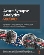
- Before we get started, let's upload the data from the Kaggle New York yellow taxi trip data dataset to the Azure Data Lake Storage Gen2 (ADLS2) storage container named taxistagingdata. You can download the dataset to your local machine and upload it to the Azure storage container, as shown in Figure 1.1:
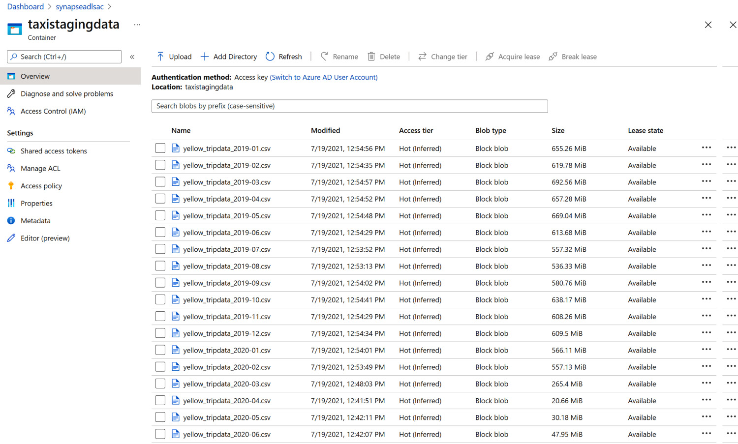
Figure 1.1 – The New York taxi dataset
- Let's create a table to load the data from the data lake storage. You can use SQL Server Management Studio (SSMS) to run the following queries against the SQL pool that you have created:
CREATE SCHEMA [NYCTaxi];
IF NOT EXISTS (SELECT * FROM sys.objects WHERE NAME = 'TripsStg' AND TYPE = 'U')
CREATE TABLE [NYCTaxi].[TripsStg]
(
VendorID nvarchar(30),
tpep_pickup_datetime nvarchar(30),
tpep_dropoff_datetime nvarchar(30),
passenger_count nvarchar(30),
trip_distance nvarchar(30),
RatecodeID nvarchar(30),
store_and_fwd_flag nvarchar(30),
PULocationID nvarchar(30),
DOLocationID nvarchar(30),
payment_type nvarchar(30),
fare_amount nvarchar(10),
extra nvarchar(10),
mta_tax nvarchar(10),
tip_amount nvarchar(10),
tolls_amount nvarchar(10),
improvement_surcharge nvarchar(10),
total_amount nvarchar(10)
)
WITH
(
DISTRIBUTION = ROUND_ROBIN,
HEAP
)
- Use the COPY INTO command to load the data from ADLS2. This helps by reducing multiple steps in the data loading process and its complexity:
COPY INTO [NYCTaxi].[TripsStg]
FROM 'https://mystorageaccount.blob.core.windows.net/myblobcontainer/*.csv'
WITH
(
FILE_TYPE = 'CSV',
CREDENTIAL=(IDENTITY= 'Shared Access Signature', SECRET= '<Your_Account_Key>'),
IDENTITY_INSERT = 'OFF'
)
GO
Next, let's look at using PolyBase.
Loading data using PolyBase
In this section, we will use PolyBase technology to load data to Synapse SQL pool. PolyBase will help in connecting external data sources, such as ADLS2 or Azure Blob storage. The PolyBase command syntax is like T-SQL, so it's easy to understand and learn this new technology without much effort:
- Create the master key and credentials, as shown in the following code block:
CREATE MASTER KEY;
--Credential used to authenticate to External Data Source
CREATE DATABASE SCOPED CREDENTIAL AzureStorageCredential
WITH
IDENTITY = 'polybaseuser',
SECRET = '<Access Key>'
;
- Create the external data source, pointing to ADLS/Azure Blob storage:
CREATE EXTERNAL DATA SOURCE NYTBlob
WITH
(
TYPE = Hadoop,
LOCATION = 'wasbs://myblobcontainer @myaccount.blob.core.windows.net/',
CREDENTIAL = AzureStorageCredential
);
Create the external file format using below query
CREATE EXTERNAL FILE FORMAT csvstaging
WITH (
FORMAT_TYPE = DELIMITEDTEXT,
FORMAT_OPTIONS (
FIELD_TERMINATOR = ',',
STRING_DELIMITER = '',
USE_TYPE_DEFAULT = False,
FIRST_ROW = 2
)
);
- Create the schema and external table. Make sure to specify the location, data source, and file format, which were previously created:
CREATE SCHEMA [NYTaxiSTG];
CREATE EXTERNAL TABLE [NYTaxiSTG].[Trip]
(
[VendorID] varchar(10) NULL,
[tpep_pickup_datetime] datetime NOT NULL,
[tpep_dropoff_datetime] datetime NOT NULL,
[passenger_count] int NULL,
[trip_distance] float NULL,
[RateCodeID] int NULL,
[store_and_fwd_flag] varchar(3) NULL,
[PULocationID] int NULL,
[DOLocationID] int NULL,
[payment_type] int NULL,
[fare_amount] money NULL,
[extra] money NULL,
[mta_tax] money NULL,
[tip_amount] money NULL,
[tolls_amount] money NULL,
[improvement_surcharge] money NULL,
[total_amount] money NULL,
[congestion_surcharge] money NULL
)
WITH
(
LOCATION = '/',
DATA_SOURCE = NYTBlob,
FILE_FORMAT = csvstaging,
FORMAT_OPTIONS (FIELD_TERMINATOR = ','),
REJECT_TYPE = value,
REJECT_VALUE = 0
);
- Check the data and table structure in SSMS connecting with the SQL pool, as shown here:
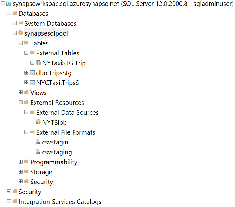
Figure 1.2 – SSMS screen
Finally, let's see the ADF method.
Loading data using ADF
ADF gives you the option to perform a data sink using three different options: PolyBase, the Copy command, and bulk insert using a dynamic pipeline. For a quick-start guide to creating a data factory using the Azure portal, you can refer to https://docs.microsoft.com/en-us/azure/data-factory/quickstart-create-data-factory-portal.
OK, let's start:
- Create and define the pipeline and use the Copy data activity.
- Define the source as the ADLS2 container where the data files were uploaded.
- Define the sink as the Synapse Analytics SQL pool.

Figure 1.3 – ADF pipeline for Copy data
We have seen the three different ways of loading data to Azure Synapse. Each of them has its own relevance. We will see how to choose which one is appropriate for your task in the How it works… section.
How it works…
To choose the best method of data loading, it is very important to understand what we are loading. Some of the key aspects we need to consider include the following:
- What does our data source look like?
- What is the format of our data source?
- How big is our dataset?
- How big is the data file size?
- How much transformation do we need to perform?
- How frequently do we want to load the data?
- Does it require incremental load or is it a full load?
We have seen the three different methods of data loading and have a fair idea of how to use each method. We will go through each method one by one and learn the benefits and considerations for data loading.
DWUs
We are assuming that you already know a bit about Data Warehouse Units (DWUs). If not, you can refer to this page to learn more: https://docs.microsoft.com/en-us/azure/synapse-analytics/sql-data-warehouse/what-is-a-data-warehouse-unit-dwu-cdwu.
The use of the COPY command gives the developer the most flexible way of loading data with numerous advantages and benefits, such as the ability to do the following:
- Execute a single T-SQL statement without having to create any additional database objects.
- Flexibly define a custom row terminator for CSV files.
- Easily use SQL Server date formats for CSV files.
- Specify a custom row terminator for CSV files.
- Specify wildcards and multiple files in the storage location path.
- Parse and load CSV files where delimiters (string, field, and row) are escaped within string-delimited columns.
- Use a different storage account for the ERRORFILE location (REJECTED_ROW_LOCATION).
- CSV supports GZIP and Parquet supports GZIP and Snappy.
- ORC supports DefaultCodec and Snappy.
When loading multiple files, it is recommended to use the file-splitting guidelines shown in the following figure. Also, there is no need to split Parquet and ORC files because the COPY command will automatically split files.
For optimal performance, Parquet and ORC files in an Azure Storage account should be 256 MB or larger.

Figure 1.4 – File splitting based on DWU
Tip
Make sure you create new statistics once you have completed the data load to your production warehouse. Bad statistics can be a common source of poor query performance in Azure Synapse Analytics. They can lead to suboptimal Massively Parallel Processing (MPP) plans, which result in unproductive data movement.
When loading data using PolyBase technology, you can retrieve data from external data stores, which could be in ADLS, Azure Blob storage, or Hadoop. The best part of PolyBase is that it uses T-SQL-like syntax so it is very convenient for database developers to write the data loading and transformation query.
Another benefit is that PolyBase can combine both relational and non-relational data and load it into a single dataset. Since PolyBase uses the MapReduce principle, it's also one of the fastest data loading techniques on scale.
PolyBase supports data loading from UTF-8 and UTF-16 text files. The Hadoop data file formats supported are the famous Parquet, OCR, and RC File. Currently, extended ASCII, nested, and fixed-width formats are not supported. So, you can't load formats such as JSON, WinZip, or XML.
Figure 1.5 – PolyBase data loading
There's more…
Here are a few more things to consider when using PolyBase for Synapse workloads:
- The load performance of PolyBase is directly proportional to the compute DWUs.
- PolyBase automatically achieves parallelism during the data load process, so you don't have to explicitly break the input data into multiple files and issue concurrent loads, unlike some traditional loading practices.
- A single PolyBase load operation provides the best performance.
- PolyBase moves data directly from Hadoop data nodes to Synapse compute nodes using MPP architecture.
Finally, let's understand the ADF data loading mechanism. As ADF provides the most seamless way to integrate with PolyBase or create your own pipeline connecting to multiple data sources, it is very convenient for ETL developers to work on the development of an ADF data pipeline.
ADF provides an interface where developers can drag and drop to create a complex data loading end-to-end pipeline. For data sources that are PolyBase compatible, you can directly invoke the Copy activity to use the PolyBase mechanism and avoid writing complex T-SQL queries.
If your source data is not originally supported by PolyBase, the copy activity additionally provides a built-in staged copy to automatically convert data into a compatible format before using PolyBase to load the data.
ADF further enriches the PolyBase integration to support the following:
- Loading data from ADLS2 with an account key or managed identity authentication.
- To connect the data source securely, you can use and create the Azure Integration Runtime, which will eventually create an ADF Virtual Network (VNET), and the Integration Runtime will be provisioned with the managed VNET.
- With the help of a managed VNET, you don't have to worry about managing the VNET to ADF yourself. You don't need to create a subnet for the Azure Integration Runtime, which could eventually use many private IPs from your VNET and would require prior network infrastructure planning – it will be done for you.
- Managed VNETs, along with managed private endpoints, protect against data breakout.
- ADF supports private links. A private link enables you to access Azure data services, such as Azure Blob storage, Azure Cosmos DB, and Azure Synapse Analytics.
- It's recommended that you create managed private endpoints to connect to all your Azure data sources.
Achieving parallelism in data loading using PolyBase
PolyBase is the one of best data loading methods when it comes to performance after the COPY Into command. So, it's recommended to use PolyBase where it's supported or possible when it comes to parallelism.
How it achieves parallelism is similar to what a parallel data warehouse system does. There will be a control node, followed by multiple compute nodes, which are then linked to multiple data nodes. The data nodes will consist of the actual data, which will get the process by the compute nodes in parallel, and all these operations and instructions are governed by the control node.
In the following architecture diagrams, each Hadoop Distributed File System (HDFS) bridge of the service from every compute node can connect to an external resource, such as Azure Blob storage, and then bidirectionally transfer data between a SQL data warehouse and the external resource. This is fully scalable and highly robust: as you scale out your DWU, your data transfer throughput also increases.
If you look at the following architecture, all the incoming connections go through the control node to the compute nodes. However, you can increase and decrease the number of compute resources as required.
Data loading parallelization is achieved as there will be multiple compute nodes that perform multithreading to process the file and load the data as quickly as possible.

Figure 1.6 – PolyBase data loading architecture
Moving and transforming using a data flow
Azure data flows are a low-code/no-code visual transformation tool that provides data engineers with a simple interface to develop the transformation logic without writing code. Azure data flows provide flexibility to ETL developers so that they can use the drag-and-drop user experience to build the data flow from one source to another, applying various transformations.
In this recipe, we will discuss and create a data flow considering the following data flow components:
- Select
- Optimize partition type
- Derived column
- Sink to Azure Synapse
Getting ready
We will be using the same dataset that we used in a previous recipe, Choosing a data loading option. Access the New York yellow taxi trip data dataset from the ADLS2 storage container named taxistagingdata. The code can be downloaded from the GitHub repository here: https://github.com/PacktPublishing/Analytics-in-Azure-Synapse-Simplified.
Also, we will be using the same pipeline that we created in the earlier recipe here and will create a data flow.
How to do it…
Let's start:
- Go to Synapse Studio and open the Develop tab.
- Create and define a new data flow under Develop within Synapse Studio.
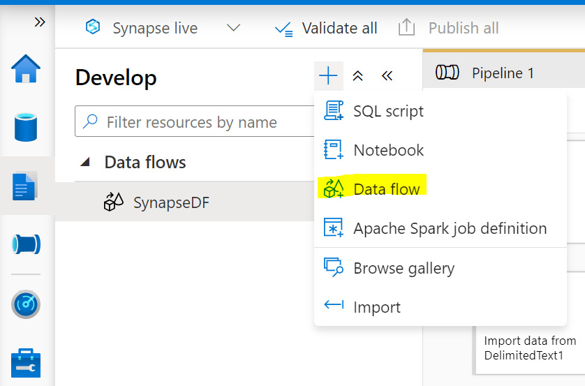
Figure 1.7 – Defining a data flow
- Define the source. In our case, it will be ADLS2, where we uploaded the files in our previous recipe.

Figure 1.8 – Source setting
- Under Optimize, please select the partition type, from a list of Round Robin, Hash, Dynamic Range, Fixed Range, or Key.

Figure 1.9 – Setting the partition type
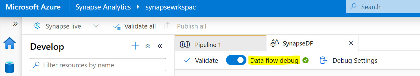
Figure 1.10 – Data flow debug mode on
- You can use the different transformations, schema modifiers, and so on. I have used derived column in our example to get the totalfare = tip_amount + tolls_amount result.

Figure 1.11 – Data flow transformation
- Define the sink/destination to load the data. In our case, it will be the Azure Synapse pool database.

Figure 1.12 – Sink data flow

Figure 1.13 – Publish data flow
- Create a pipeline to call the existing flow that we have just created. Click on the integrate icon on the left and add a new pipeline.

Figure 1.14 – Create pipeline

Figure 1.15 – Creating and calling a data flow pipeline
Now we have a customized pipeline that we can reuse any time.
How it works…
This is one way you can use Azure data flows to create data pipelines and consume data. The main purpose of having a flow pipeline is that you can call, schedule, or trigger this at any time so that it can be part of the data load schedule.
You can also take advantage of the end-to-end monitoring of a pipeline so that it is easier for you or another developer to debug it if there are any data loading issues or failures.
Adding a trigger to a data flow pipeline
In the Moving and transforming data using a data flow recipe, we created a data flow and manually performed the execution of pipelines, also known as on-demand execution, to test the functionality and the results of the pipelines that we created. However, in a production scenario, we need the pipeline to be triggered at a specific time as per our data loading strategy. We need an automated method to schedule and trigger these pipelines, which is done using triggers.
The schedule trigger is used to execute ADF pipelines or data flows on a wall-clock schedule.
Getting ready
Make sure you have the pipeline demonstrated in the previous recipes created and published.
The data flow is created by calling the existing pipeline, as we did in the previous recipe.
How to do it…
Let's begin:
- An ADF trigger can be created under the Manager page, by clicking on the Add trigger | New/Edit | Create Trigger option from the triggers window, as shown in the following screenshot:
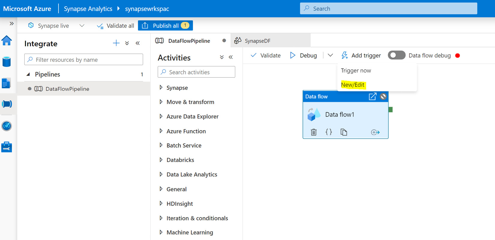
Figure 1.16 – Adding a trigger
The schedule trigger executes the pipeline on a wall-clock schedule, the tumbling window trigger executes the pipeline at a periodic interval and retains the pipeline state, and the event-based trigger responds to a blob-related event.
- A scheduled trigger will have a start date, the time zone that will be used in the schedule, the end date of the trigger, and the frequency of the trigger (this is optional), with the ability to configure the trigger frequency to be called every specific number of minutes or hours, as shown in the following screenshot:
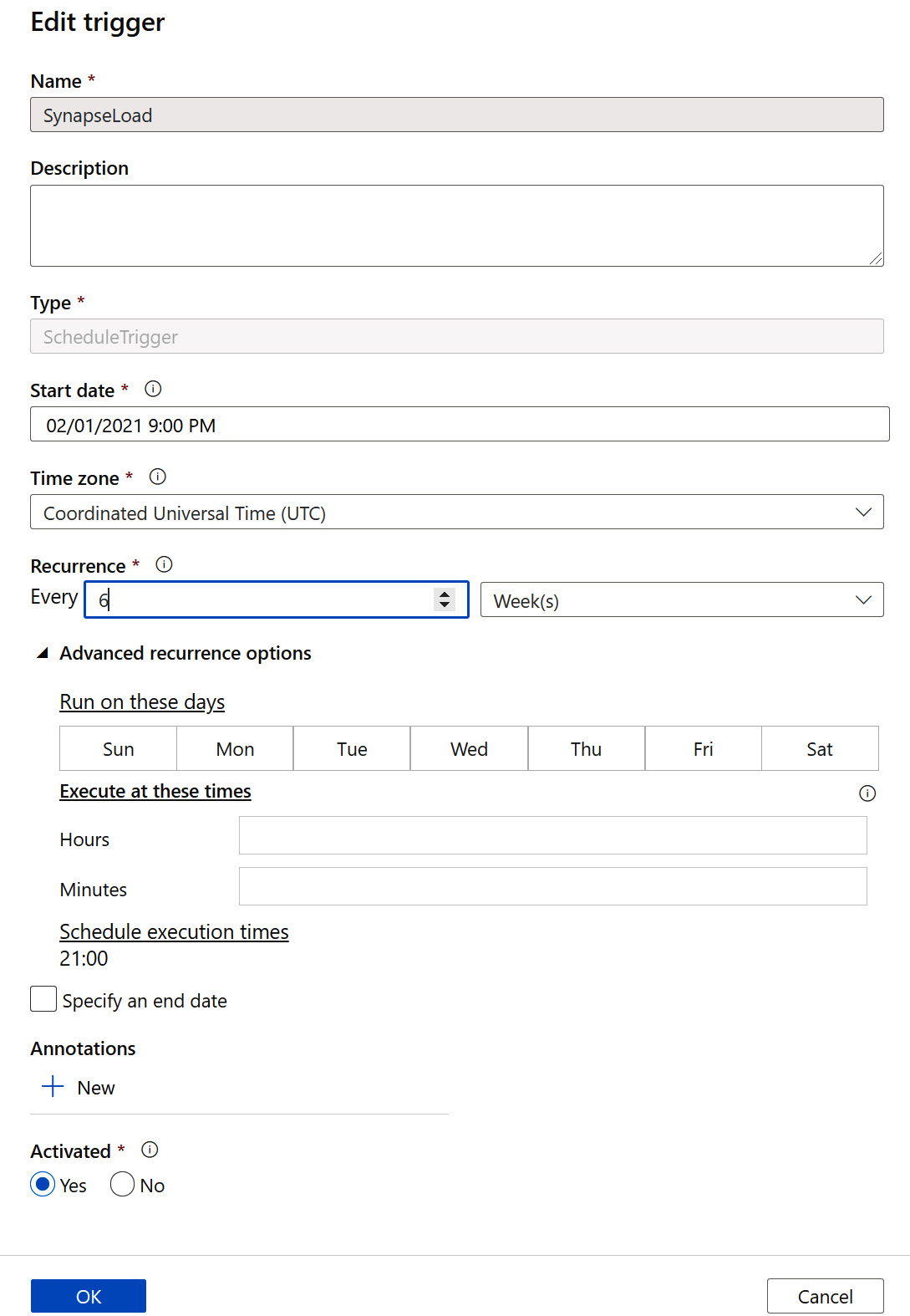
Figure 1.17 – Schedule-based trigger
- An event-based trigger executes pipelines in response to a blob-related event, such as creating or deleting a blob file, in Azure Blob storage, as shown in Figure 1.18:

Figure 1.18 – Event-based trigger
How it works…
A trigger execution is typically initiated by passing the arguments to the parameters that you have created and defined in the pipeline. Every pipeline is associated with a unique pipeline run ID, which is a unique GUID that is responsible for that particular run.
Unsupported data loading scenarios
In the case of migration scenarios when migrating your database from another SQL database, there is a possibility that some of the data types are not supported on Synapse SQL.
How to do it…
In order to identify the unsupported data types in your current SQL scheme, you can use the following T-SQL query:
SELECT t.[name], c.[name], c.[system_type_id], c.[user_type_id], y.[is_user_defined], y.[name]
FROM sys.tables t
JOIN sys.columns c on t.[object_id] = c.[object_id]
JOIN sys.types y on c.[user_type_id] = y.[user_type_id]
WHERE y.[name] IN ('geography','geometry','hierarchyid','image','text','ntext','sql_variant','xml')
AND y.[is_user_defined] = 1;
There's more…
A list of the data types that are unsupported and an alternative workaround that you can use is shown in the following table. This list is from the official Microsoft documentation:

Figure 1.19 – A table showing unsupported data types
Data loading best practices
Azure Synapse Analytics has a rich set of tools and methods available to load data into SQL pool. You can load data from relational or non-relational data stores; structured or semi-structured data; on-premises systems or other clouds; in batches or streams. The loading can be done using various methods, such as with PolyBase, using the COPY into command, using ADF, or creating a data flow.
How to do it…
In this section, we'll look at some basic best practices to keep in mind as you work.
Retaining a well-engineered data lake structure
Retaining a well-engineered data lake structure allows you to know that the data you're loading regularly is consistent with the data requirements for your system.
When loading large datasets, it's recommended to use the compression capabilities of the file format. This ensures that less time is spent on the process of transferring data, using instead the power of Azure Synapse's MPP compute capabilities for decompression.
Setting a dedicated data loading account
A common error that many of us make while performing data exploration is to use the service administrator account. This account is limited to using the smallrc dynamic resource class, which can use between 3% and 25% of the resources depending on the performance level of the provisioned SQL pool.
Hence, it is best to create a dedicated account assigned to different resources classes dependent on the projected task:
- Create a login within the master database so you can connect SQL pool using SSMS:
-- Connect to master
CREATE LOGIN loader WITH PASSWORD = '<strong password>';
- Connect to the dedicated SQL pool and create a user:
-- Connect to the SQL pool
CREATE USER loader FOR LOGIN loader;
GRANT ADMINISTER DATABASE BULK OPERATIONS TO loader;
GRANT INSERT ON <yourtablename> TO loader;
GRANT SELECT ON <yourtablename> TO loader;
GRANT CREATE TABLE TO loader;
GRANT ALTER ON SCHEMA::dbo TO loader;
CREATE WORKLOAD GROUP LoadData
WITH (
MIN_PERCENTAGE_RESOURCE = 100
,CAP_PERCENTAGE_RESOURCE = 100
,REQUEST_MIN_RESOURCE_GRANT_PERCENT = 100
);
CREATE WORKLOAD CLASSIFIER [wgcELTLogin]
WITH (
WORKLOAD_GROUP = 'LoadData'
,MEMBERNAME = 'loader'
);
Handling data loading failure
The frequent Query aborted-- the maximum reject threshold was reached while reading from an external source failure error message indicates that your external data contains dirty records.
This error occurs when you meet any of the following criteria:
- If there is a mismatch between the number of columns or the data type of the column definition of the external table
- If the dataset doesn't fit the specified external file format
To handle dirty records, please make sure you have the correct definition for the external table and the external file format so that your external data fits under these definitions.
Using statistics after the data is loaded
In order to improve the query performance, one of the key things you can do is to generate statistics for your data once the data is loaded to the dedicated SQL pool.
Turn the AUTO_CREATE_STATISTICS option on for the database. This will enable SQL dedicated pool to analyze the incoming user query for any missing statistics and optimize them.
The query optimizer creates statistics for individual columns if there are any missing statistics.
To enable dedicated SQL pool on AUTO_CREATE_STATISTICS, you can execute the following command:
ALTER DATABASE <yourdwname>
SET AUTO_CREATE_STATISTICS ON
These tips should prove useful throughout the book and your Synapse experience.