Chapter 3: Processing Data Optimally across Multiple Nodes

In this chapter, we will cover the Synapse SQL architecture components that are required for running data transformation pipelines and leverage the scale-out capabilities to distribute computational data processing and transformation across multiple nodes. Synapse SQL architecture is designed in such a way that the compute is totally separated from storage and, as needed, the compute can be scaled independently of the data. Since compute and data are separated, the queries handled by compute enable massively parallel processing, performance, and greater speed in retrieving the data.

We will cover the following recipes:

• Working with the resource consumption model of Synapse SQL
• Optimizing analytics with dedicated SQL pool and working on data distribution
• Working with serverless SQL pool
• Processing and querying very large datasets
• Script for statistics in Synapse SQL

Working with the resource consumption model of Synapse SQL

In this section, we will understand the architecture components of Synapse SQL, the definition of analytical storage, and how storage and compute work together to distribute computational processing of data across multiple nodes. Then we will cover the resource consumption model of Synapse SQL, which enables you to choose the right model for your analytical storage and queries.

Architecture components of Synapse SQL

Synapse SQL has two main types of SQL pools for analytical storage:

• Dedicated SQL
• Serverless SQL

Dedicated SQL

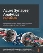
The Synapse dedicated SQL underlying architecture is node-based. Applications issue T-SQL to a control node, which is considered a single-entry point for Synapse SQL.

The Synapse SQL control node utilizes a massively parallel processing distributed query engine to optimize queries for parallel processing and then splits them into different sets of queries for each compute node for parallel execution.

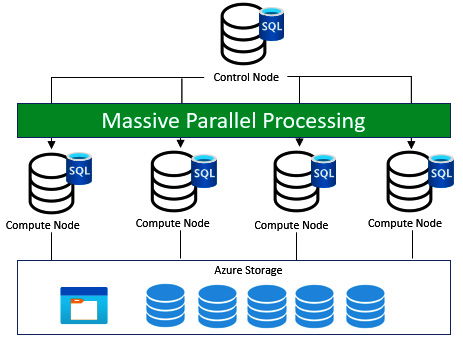
Figure 3.1 – Dedicated SQL pool under the hood

The data that is required for compute nodes is stored in Azure Storage. The Data movement service (DMS) is an internal system-level service that helps you move data across nodes and compute nodes run queries in parallel, returning results to the application that issued the T-SQL commands.

Serverless SQL

The scaling of compute resources for serverless SQL is done automatically according to query and resourcing requirements.

Serverless SQL pool has a control node that utilizes the distributed query processing engine, which orchestrates the distributed parallel execution of queries issued by the user. It splits larger queries into smaller queries, which are executed by compute nodes and orchestrated by the control node. Data is stored in Azure Storage and the compute node processes the data in storage with queries, which provides the necessary results.

Figure 3.2 – Serverless SQL pool under the hood

There are differences between serverless SQL pool and dedicated SQL pool in how and where the data resides. Serverless SQL pool queries data lake files directly from Azure Storage, whereas dedicated SQL pool queries ingest data from data lake files in Azure Storage to SQL in the compute node. Data that is ingested into dedicated SQL pool will be sharded into distributions for optimal performance. The sharding patterns are as listed:

• Hash
• Round robin
• Replicate

Sharding pattern or distribution

Dedicated SQL pool in a compute node will split into 60 smaller queries that run in parallel. Each of the 60 smaller queries runs on one of the distribution or sharding patterns. Dedicated SQL pool has one distribution per compute node. If we choose Dedicated SQL pool with minimum compute resources, then all the data distribution will run on one compute node.

• Hash distribution: This delivers the highest performance for joins and aggregations on larger tables. Dedicated SQL pool uses the hash function to assign each row to a distribution. One of the columns will be defined as the distribution column. The hash functions use values in the distribution column and assign each row to a distribution.
• Round-robin distribution: This delivers fast performance when used as a staging table, particularly for loads. A round-robin distributed table distributes data evenly across the table. This distribution is random and round robin requires shuffling of data, which increases the latency on query retrieval.
• Replicated tables: This delivers the fastest query performance for smaller tables. The table is replicated on each compute node and a full copy of the table is cached. Since the table is replicated, transferring data between the compute nodes is not required when we do a join or aggregation. The performance is outstanding for smaller tables but it adds more overhead when writing data and hence is not suitable for larger tables.

Resource consumption

The following are the resource consumption models for Synapse SQL:

• Serverless SQL pool: A pay-per-query service where resources are increased or decreased automatically based on consumption.
• Dedicated SQL pool: The unit of scale is an abstraction of compute power and is called a data warehouse unit. The analytical storage is a combination of compute, memory, and IO, bundled as data warehouse units.

Increasing the data warehouse units would do the following:

• Increase the performance of scans, aggregations, and CREATE TABLE AS SELECT (CTAS) statements.
• Increase the number of readers and writers for PolyBase load operations.
• Increase the capacity in running concurrent queries and increase concurrency slots.

Figure 3.3 – Table showing data warehouse units

Optimizing analytics with dedicated SQL pool and working on data distribution

In this section, we will understand the in-depth details of dedicated SQL pool for optimizing analytics on a larger dataset. We need to understand the basics of column storage; know when to use round robin, hash distribution, and replicated data distributions; know when to partition a table and check for data skew and space usage; know the best practices and how to effectively use workload management for dedicated SQL pool.

Understanding columnstore storage details

A columnar store is logically organized as a table with rows and columns. It is physically stored in a column-wise data format. Generally, a rowgroup (group of rows) is compressed in columnar store format. A rowgroup consists of the maximum number of rows per rowgroup. The columnstore index slices the table into rowgroups and then compresses the rowgroups column-wise.

A clustered columnstore index is the primary storage for the entire table and it is useful for data warehousing and analytics workloads. It is used to store fact tables and large dimension tables. It improves query performance and data compression by 10 times compared to a nonclustered index.

A nonclustered index is a secondary index that is created on a rowstore table and is useful for real-time operational analytics in an Online transaction processing (OLTP) workload.

A columnstore index provides a high level of data compression and significantly reduces data warehouse storage costs. Columnstore indexes are the preferred data storage format for data warehousing and analytics workloads. 

Knowing when to use round-robin, hash-distributed, and replicated distributions

A distributed table is actually a single table outwardly but rows are stored in 60 distributions. The distribution of rows either uses hash or the round-robin algorithm. Hash is used for large fact tables. Round robin is useful for improving loading speed. Replicated tables are used for smaller datasets.

To choose between three distribution options, for all design scenarios, consider asking yourself the following set of questions:

• What is the size of the table?
• What is the frequency at which we access the table and refresh the table?
• Are we going to use fact and dimension tables in dedicated SQL pool?

If the answers to the preceding questions are as follows, then consider using hash distribution:

• Larger fact tables and the table size is more than 2 GB on disk.
• Data will be refreshed frequently and accessed by concurrent users for reporting. It has frequent Create, Read, Update, Delete, and List (CRUDL) operations.
• Both fact and dimension tables are needed in dedicated SQL pool.

Hash distribution

Hash distribution distributes table rows across the compute nodes by using a deterministic hash function, which assigns each row one distribution in each compute node. All identical values will be stored in the same distribution. SQL Analytics will store the location of the row, and this will help to minimize data movement, which improves query performance. It works out well if we have a very large numbers of rows.

Round-robin distribution

Round robin distributes table rows evenly across all distributions. Rows with equal values will not be assigned to the same distribution and assignment is completely random. Hence there are more data movement operations to organize the data and shuffling frequently hits the performance. Consider using round robin for the following scenarios:

• None of the columns are suitable candidates for hash distribution.
• The table does not share a common join key and there is no join key.
• When we need to use this for temporary staging.

Replicated tables

Replicated tables hold a full copy of the table on the compute node. Replicating a table removes the need to transfer data between compute nodes. Since the table has multiple copies, a replicated table works out if the table size is less than 2 GB compressed.

Consider using a replicated table when the following applies:

• The table size is less than 2 GB irrespective of the number of rows.
• The table used in joins requires data movement. If one of the tables is small, consider a replicated table.

Replicated tables will not provide the best query performance in the following scenarios:

• The table has frequent CRUDL operations. This slows down the performance.
• The SQL pool is scaled frequently. Scaling requires us to copy the replicated tables frequently to the compute node, which slows the performance.
• The table has many columns but read operations are targeted only to a small number of columns. It would be effective to distribute the table and create an index on frequently queried columns instead of using replicated tables.

Knowing when to partition a table

Table partitions help to segregate data into smaller groups of data. Mostly, they are created on the date column. Table partitioning is supported on all table types with different sets of indexes and also on different distribution types.

The benefit is that it improves query performance because it limits the scan only to qualified partitions. This avoids a full table scan and scans only a limited set of data.

A design with too many partitions can affect the performance. At least 1 million rows per distribution and partition are required for optimal compression and performance of columnstore index tables. If there are 1 million rows per distribution and a full table scan can be avoided, we recommend using partitions.

Checking for skewed data and space usage

We learned in previous sections that data should be evenly distributed across a distribution. When data is not distributed evenly, it results in data skew. If there is data skew, some processing in a compute node will take a longer time and others will finish more quickly. This is not an ideal scenario and you must therefore choose your distribution column in such a way that it has many unique values, no date column, and does not contain NULL values or has only a few NULL values.

Check data skew with DBCC PDW_SHOWSPACEUSED as shown in the following line of code:

DBCC PDW_SHOWSPACEUSED('dbo.FactSales');

Data skew identification is necessary so that we can finish the processing quickly and, as in the preceding line, we need to check the tables frequently.

Best practices

We will learn a few best practices and tips that help in the design of optimized analytics for dedicated SQL pool.

Batching the insert statements together will reduce the number of round trips and improve efficiency. If there are larger volumes of data that have to be loaded into dedicated SQL pool, choose PolyBase and select hash distribution. While partitioning helps in query performance, too many partitions can be detrimental to performance.

INSERT, UPDATE, and DELETE statements always run in a transaction. The transaction is rolled back if there is a failure. Minimize the transaction size to reduce long rollbacks, which is achieved by dividing these statements into parts. For instance, if an UPDATE statement is expected to get completed in 1 hour, we can break this into four equal parts so that each part takes 15 minutes to complete. Any error in the middle of a transaction will have a quicker rollback.

Reduce the number of query results and use the top statement to return only a specific set of rows. Designing the smallest possible column size is helpful because the overall table will be smaller and the query results will also be smaller. Temporary tables should be used for loading transient data.

Designing a columnstore index for tables of more than 60 million rows is a good solution. When we partition data, each partition is expected to have 1 million rows to benefit from a columnstore index. Hence a table with 100 partitions should have 100 million rows to benefit from columnstore indexing (since by default there will be 60 distributions and 100 partitions, which actually need 1 million rows).

Workload management for dedicated SQL pool

Dedicated SQL pool offers workload management with the following three concepts:

• Workload classification
• Workload importance
• Workload isolation

This enables us to maintain query performance at an optimized level throughout. We can choose an appropriate capacity for DWU and it offers memory, distribution, and concurrency limits based on DWU.

Workload classification involves classifying the workload group based on loading the data with INSERT, UPDATE, and DELETE and then querying the data with Select. A data warehousing solution will have one kind of workload policy for loads that are classified as a high-resource class, which requires more resources, and a different workload policy for Select queries where loading might take precedence compared to querying. The first step is to classify the workload into a workload group.

Workload importance involves the order or priority in which a request gets access.

Workload isolation involves reserving resources for a workload group. We can define the quantity of resources that are assigned based on resource classes.

All these workload groups have a configuration for query timeout and requests. The workload groups require constant monitoring and management to maintain optimal query performance.

Working with serverless SQL pool

Azure Synapse Analytics has serverless SQL pool endpoints that are primarily used to query data in Azure Data Lake (Parquet, Delta Lake, delimited text formats), Azure Cosmos DB, and Dataverse.

We can access the data using T-SQL queries without the need to copy and load data in a SQL store through serverless SQL pool. Serverless SQL pool is ideally a wrapper service for interactive querying and distributed data processing for large-scale analysis of big data systems. It is a completely serverless and managed service offering from Microsoft Azure, built with fault tolerance, high reliability, and high performance for larger datasets.

Serverless SQL pool is suitable for the following scenarios:

• Basic exploration and discovery where data in Azure Data Lake Storage (ADLS)with different formats such as Parquet, CSV, Delta, and JSON can be used to derive insights.
• A relational abstraction layer on top of raw data without transformation, allowing you to get an up-to-date view of data. This will be created on top of Azure Storage and Azure Cosmos DB.
• Simple, scalable, and performance-efficient data transformation with T-SQL.

In this recipe, we will learn how to explore data from Parquet stored in ADLS Gen 2 with serverless SQL pool.

Getting ready

We will be using a public dataset for our scenario. This dataset will consist of New York yellow taxi trip data: this includes attributes such as trip distances, itemized fares, rate types, payment types, pick-up and drop-off dates and times, driver-reported passenger counts, and pick-up and drop-off locations. We will be using this dataset throughout this recipe to demonstrate various use cases.

• To get the dataset, you can go to the following URL: https://www.kaggle.com/microize/newyork-yellow-taxi-trip-data-2020-2019.
• The code for this recipe can be downloaded from the GitHub repository: https://github.com/PacktPublishing/Analytics-in-Azure-Synapse-Simplified.

Let's get started.

How to do it…

Let's first create our Synapse Analytics workspace and then create serverless SQL pool on top of it. We will upload a Parquet file and explore it with serverless SQL.

Synapse Analytics workspace creation requires us to create a resource group or access to an existing resource group with owner permissions. Let's use an existing resource group where you will find owner permissions for the user:

1. Log in to the Azure portal: https://portal.azure.com/#home.
2. Search for synapse on the Microsoft Azure page and then navigate to Azure Synapse Analytics.
3. Select Azure Synapse Analytics.

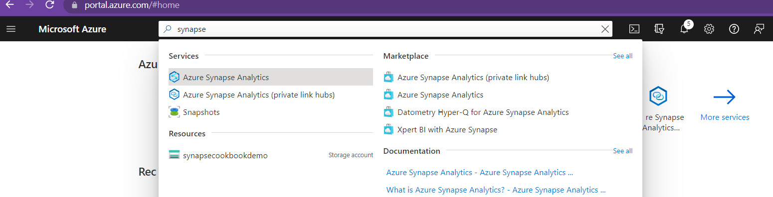
Figure 3.4 – Search for Synapse Analytics

4. Create an Azure Synapse Analytics workspace using the Create button or the Create Synapse workspace button.

Figure 3.5 – Create Synapse Analytics workspace

5. On the Basics tab, enter the resource group workspace name as synapsecookbook.
6. Associate it with already created ADLS Gen 2 account name and the container.

Figure 3.6 – Create Synapse workspace Basics tab

7. Enter the SQL administrator password to access the Synapse workspace upon login.

Figure 3.7 – Create Synapse workspace Security tab

8. Review and create the workspace.
9. Go to the existing Synapse Analytics workspace and navigate to Synapse Studio.

Figure 3.8 – Synapse Studio

10. Create a Serverless SQL database in Synapse Studio.
    

Figure 3.9 – Create serverless SQL pool

11. Upload the NYCTripSmall.parquet file in any existing storage account.
12. Query the Parquet file as external storage with T-SQL as follows:

    select top 10 *

    from openrowset(

        bulk 'abfss://[email protected]/NYCTripSmall.parquet',

        format = 'parquet') as rows

That completes the recipe!

There's more…

Serverless SQL pool allows us to query files in ADLS. It does not have storage like dedicated SQL pool or ingestion capabilities. The following list suggests some best practices for serverless SQL pool:

• Always co-locate client applications such as Power BI in the same region as serverless SQL pool for good performance.
• Co-locate ADLS, Cosmos DB, and serverless SQL pool in the same region.
• Optimize storage using partitioning and files in Azure Storage between 100 MB and 1 GB.
• Cache results on the client side (Power BI or Azure Analysis Services (AAS)) and refresh it frequently. Serverless SQL pool is not suitable for complex queries or processing a large amount of data in Power BI DirectQuery mode.

Processing and querying very large datasets

Synapse SQL uses distributed query processing, the data movement service, and scale-out architecture, leveraging the advantages of the scalability and flexibility of compute and storage. Data transformation is not required prior to loading it to Synapse SQL. We need to use the built-in massively parallel processing capabilities of Synapse, load data in parallel, and then perform the transformation.

Loading data using PolyBase external tables and COPY SQL statements is considered one of the fastest, most reliable, and scalable ways of loading data. We can use external data stored in ADLS and Azure Blob storage, and load data using the COPY statement. This data is then loaded to production tables and exposed as views, which creates a query view for the client applications to derive meaningful business insights.

Getting ready

We will be performing a series of steps in order to extract, load, and create a materialized view of data for larger datasets. The Azure documentation has the syntax for all the steps, which should be referred to for actual implementation:

• https://docs.microsoft.com/en-us/azure/synapse-analytics/sql/develop-tables-external-tables?tabs=hadoop#create-external-data-source
• https://docs.microsoft.com/en-us/azure/synapse-analytics/sql/develop-tables-external-tables?tabs=hadoop#create-external-file-format
• https://docs.microsoft.com/en-us/azure/synapse-analytics/sql/develop-tables-external-tables?tabs=hadoop#create-external-table
• https://docs.microsoft.com/en-us/sql/t-sql/statements/copy-into-transact-sql?view=azure-sqldw-latest

How to do it…

Let's now dive deep into the step-by-step process of extracting, loading, and creating the materialized view of data:

1. Extract the source data into text, Parquet, or CSV files. Let's take an example where the source data is in Oracle. Use Oracle's built-in wizards or third-party tools to move the data from Oracle to delimited text or CSV files. Converting to Parquet will be useful and is supported in Synapse SQL. Load the data from UTF-8 and UTF-16 as delimited text or CSV files.
2. Load the data into Azure Blob storage or ADLS. Synapse data integration or Azure Data Factory can be used to load the text files created earlier or CSV files into Azure Blob storage or ADLS. If we are loading this larger dataset on-premises, it is highly recommended to have Azure ExpressRoute or Site-to-Site VPN established between on-premises and Azure.
3. Prepare the data for loading. We need to prepare the data before we load it to Synapse SQL tables.
4. Define the tables. First, define the tables before loading them to dedicated SQL pool. We can define external tables in dedicated SQL pool before loading. External tables are similar to database views. These external tables will have the table schema and data that is stored outside dedicated SQL pool.

There are several different ways of defining tables, which are listed as follows:

• CREATE EXTERNAL DATA SOURCE
• CREATE EXTERNAL FILE FORMAT
• CREATE EXTERNAL TABLE

5. Load the data into Synapse SQL using PolyBase or the COPY statement. Data is loaded to staging tables. The options for loading are as follows:
   • COPY statement: The following code is the sample for loading Parquet files into Synapse SQL:

     COPY INTO test_parquet

     FROM 'https://myaccount.blob.core.windows.net/myblobcontainer/folder1/*.parquet'

     WITH (

         FILE_FORMAT = myFileFormat,

         CREDENTIAL=(IDENTITY= 'Shared Access Signature', SECRET='<Your_SAS_Token>')

     )

6. Configure PolyBase in Azure Data Factory or Synapse data integration.
7. Transform the data and move it to production tables. The data is in staging tables now and you can perform transformations with a T-SQL statement and move data into the production table. The INSERT INTO ... SELECT statement moves the data from the staging table to the production table.
8. Create materialized views for consumption. Materialized views are views where data gets automatically updated as data changes in underlying production tables. Views significantly improve the performance of complex queries (typically queries with lot of joins, aggregations, and complex joins) and offer simple maintenance.

Processing and querying large datasets requires us to load them in parallel, process them with massively parallel processing clusters, and create materialized views that refresh the data automatically. These materialized views will be used by the reporting tool for dashboards and deriving insights.

Script for statistics in Synapse SQL

Once the data is loaded into a dedicated SQL pool, statistics collection from data is very important for continuous query optimization. The dedicated SQL pool query optimizer is a cost-based optimizer that compares query plans and chooses the plan with the lowest cost. The dedicated SQL pool engine will analyze incoming user queries where the statistics are constantly analyzed and the database AUTO_CREATE_STATISTICS option is set to ON. If the statistics are not available, then the query optimizer will create statistics on individual columns.

How to do it…

By default, statistics creation is turned on. Check the data warehouse configuration for AUTO_CREATE_STATISTICS using the following command:

SELECT name, is_auto_create_stats_on

FROM sys.databases

Enable statistics with the following command:

ALTER DATABASE <datawarehousename>

SET AUTO_CREATE_STATISTICS ON

Once the statistics command is received, it will trigger the automatic creation of statistics for the following statements:

• SELECT
• INSERT-SELECT
• CTAS
• UPDATE
• DELETE
• EXPLAIN

Creating and updating statistics

The following command is used to create and update statistics for a table with a set of columns or all columns:

CREATE STATISTICS [statistics_name]   ON [schema_name].[table_name]([column_name]);

UPDATE STATISTICS [schema_name].[table_name]([stat_name]);

UPDATE STATISTICS [schema_name].[table_name];

Serverless SQL pool supports the automatic creation of statistics only for Parquet files. For CSV files, statistics have to be created manually.

We can create stored procedures and views with all statistics enabled. These stored procedures can be used to automatically execute on the creation and updating of statistics of selected columns in tables.

There's more…

System views and functions are used to get information on statistics. STATS_DATE() allows you to view the statistics created or updated. The following table lists the system views that we can use to get relevant information on statistics:

Figure 3.10 – Table providing information on system views