13
TOOLS OF PARAMETER ESTIMATION: THE PDF, CDF, AND QUANTILE FUNCTION

In this part so far, we’ve focused heavily on the building blocks of the normal distribution and its use in estimating parameters. In this chapter, we’ll dig in a bit more, exploring some mathematical tools we can use to make better claims about our parameter estimates. We’ll walk through a real-world problem and see how to approach it in different ways using a variety of metrics, functions, and visualizations.

This chapter will cover more on the probability density function (PDF); introduce the cumulative distribution function (CDF), which helps us more easily determine the probability of ranges of values; and introduce quantiles, which divide our probability distributions into parts with equal probabilities. For example, a percentile is a 100-quantile, meaning it divides the probability distribution into 100 equal pieces.

Estimating the Conversion Rate for an Email Signup List

Say you run a blog and want to know the probability that a visitor to your blog will subscribe to your email list. In marketing terms, getting a user to perform a desired event is referred to as the conversion event, or simply a conversion, and the probability that a user will subscribe is the conversion rate.

As discussed in Chapter 5, we would use the beta distribution to estimate p, the probability of subscribing, when we know k, the number of people subscribed, and n, the total number of visitors. The two parameters needed for the beta distribution are α, which in this case represents the total subscribed (k), and β, representing the total not subscribed (n – k).

When the beta distribution was introduced, you learned only the basics of what it looked like and how it behaved. Now you’ll see how to use it as the foundation for parameter estimation. We want to not only make a single estimate for our conversion rate, but also come up with a range of possible values within which we can be very confident the real conversion rate lies.

The Probability Density Function

The first tool we’ll use is the probability density function. We’ve seen the PDF several times so far in this book: in Chapter 5 where we talked about the beta distribution; in Chapter 9 when we used PDFs to combine Bayesian priors; and once again in Chapter 12, when we talked about the normal distribution. The PDF is a function that takes a value and returns the probability of that value.

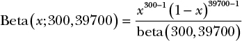
In the case of estimating the true conversion rate for your email list, let’s say for the first 40,000 visitors, you get 300 subscribers. The PDF for our problem is the beta distribution where α = 300 and β = 39,700:

We’ve spent a lot of time talking about using the mean as a good estimate for a measurement, given some uncertainty. Most PDFs have a mean, which we compute specifically for the beta distribution as follows:

This formula is relatively intuitive: simply divide the number of outcomes we care about (300) by the total number of outcomes (40,000). This is the same mean you’d get if you simply considered each email an observation of 1 and all the others an observation of 0 and then averaged them out.

The mean is our first stab at estimating a parameter for the true conversion rate. But we’d still like to know other possible values for our conversion rate. Let’s continue exploring the PDF to see what else we can learn.

Visualizing and Interpreting the PDF

The PDF is usually the go-to function for understanding a distribution of probabilities. Figure 13-1 illustrates the PDF for the blog conversion rate’s beta distribution.

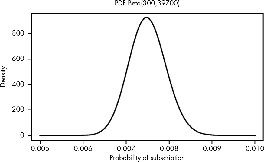
Figure 13-1: Visualizing the beta PDF for our beliefs in the true conversion rate

What does this PDF represent? From the data we know that the blog’s average conversion rate is simply

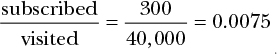
or the mean of our distribution. It seems unlikely that the conversion rate is exactly 0.0075 rather than, say, 0.00751. We know the total area under the curve of the PDF must add up to 1, since this PDF represents the probability of all possible estimates. We can estimate ranges of values for our true conversion rate by looking at the area under the curve for the ranges we care about. In calculus, this area under the curve is the integral, and it tells us how much of the total probability is in the region of the PDF we’re interested in. This is exactly like how we used integration with the normal distribution in the prior chapter.

Given that we have uncertainty in our measurement, and we have a mean, it could be useful to investigate how much more likely it is that the true conversion rate is 0.001 higher or lower than the mean of 0.0075 we observed. Doing so would give us an acceptable margin of error (that is, we’d be happy with any values in this range). To do this, we can calculate the probability of the actual rate being lower than 0.0065, and the probability of the actual rate being higher than 0.0085, and then compare them. The probability that our conversion rate is actually much lower than our observations is calculated like so:

Remember that when we take the integral of a function, we are just summing all the little pieces of our function. So, if we take the integral from 0 to 0.0065 for the beta distribution with an α of 300 and a β of 39,700, we are adding up all the probabilities for the values in this range and determining the probability that our true conversion rate is somewhere between 0 and 0.0065.

We can ask questions about the other extreme as well, such as: how likely is it that we actually got an unusually bad sample and our true conversion rate is much higher, such as a value greater than, say, 0.0085 (meaning a better conversion rate than we had hoped)?

Here we are integrating from 0.0085 to the largest possible value, which is 1, to determine the probability that our true value lies somewhere in this range. So, in this example, the probability that our conversion rate is 0.001 higher or more than we observed is actually more likely than the probability that it is 0.001 less or worse than observed. This means that if we had to make a decision with the limited data we have, we could still calculate how much likelier one extreme is than the other:

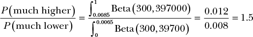
Thus, it’s 50 percent more likely that our true conversion rate is greater than 0.0085 than that it’s lower than 0.0065.

Working with the PDF in R

In this book we’ve already used two R functions for working with PDFs, dnorm() and dbeta(). For most well-known probability distributions, R supports an equivalent dfunction() function for calculating the PDF.

Functions like dbeta() are also useful for approximating the continuous PDF—for example, when you want to quickly plot out values like these:

xs <- seq(0.005,0.01,by=0.00001)
xs.all <- seq(0,1,by=0.0001)
plot(xs,dbeta(xs,300,40000-300),type='l',lwd=3,
     ylab="density",
     xlab="probability of subscription",
     main="PDF Beta(300,39700)")

In this example code, we’re creating a sequence of values that are each 0.00001 apart—small, but not infinitely small, as they would be in a truly continuous distribution. Nonetheless, when we plot these values, we see something that looks close enough to a truly continuous distribution (as shown earlier in Figure 13-1).

Introducing the Cumulative Distribution Function

The most common mathematical use of the PDF is in integration, to solve for probabilities associated with various ranges, just as we did in the previous section. However, we can save ourselves a lot of effort with the cumulative distribution function (CDF), which sums all parts of our distribution, replacing a lot of calculus work.

The CDF takes in a value and returns the probability of getting that value or lower. For example, the CDF for Beta(300,397000) when x = 0.0065 is approximately 0.008. This means that the probability of the true conversion rate being 0.0065 or less is 0.008.

The CDF gets this probability by taking the cumulative area under the curve for the PDF (for those comfortable with calculus, the CDF is the anti-derivative of the PDF). We can summarize this process in two steps: (1) figure out the cumulative area under the curve for each value of the PDF, and (2) plot those values. That’s our CDF. The value of the curve at any given x-value is the probability of getting a value of x or lower. At 0.0065, the value of the curve would be 0.008, just as we calculated earlier.

To understand how this works, let’s break the PDF for our problem into chunks of 0.0005 and focus on the region of our PDF that has the most probability density: the region between 0.006 and 0.009.

Figure 13-2 shows the cumulative area under the curve for the PDF of Beta(300,39700). As you can see, our cumulative area under the curve takes into account all of the area in the pieces to its left.

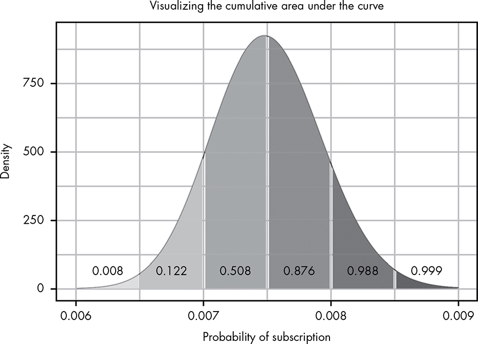
Figure 13-2: Visualizing the cumulative area under the curve

Mathematically speaking, Figure 13-2 represents the following sequence of integrals:

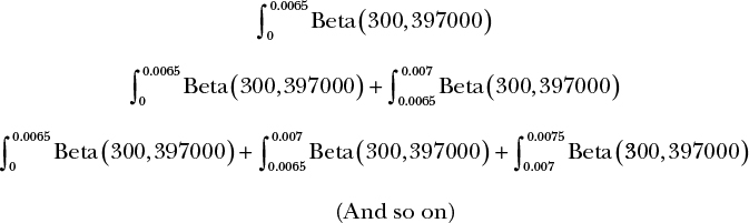
Using this approach, as we move along the PDF, we take into account an increasingly higher probability until our total area is 1, or complete certainty. To turn this into the CDF, we can imagine a function that looks at only these areas under the curve. Figure 13-3 shows what happens if we plot the area under the curve for each of our points, which are 0.0005 apart.

Now we have a way of visualizing just how the cumulative area under the curve changes as we move along the values for our PDF. Of course, the problem is that we’re using these discrete chunks. In reality, the CDF just uses infinitely small pieces of the PDF, so we get a nice smooth line (see Figure 13-4).

In our example, we derived the CDF visually and intuitively. Deriving the CDF mathematically is much more difficult, and often leads to very complicated equations. Luckily, we typically use code to work with the CDF, as we’ll see in a few more sections.

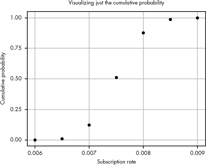
Figure 13-3: Plotting just the cumulative probability from Figure 13-2

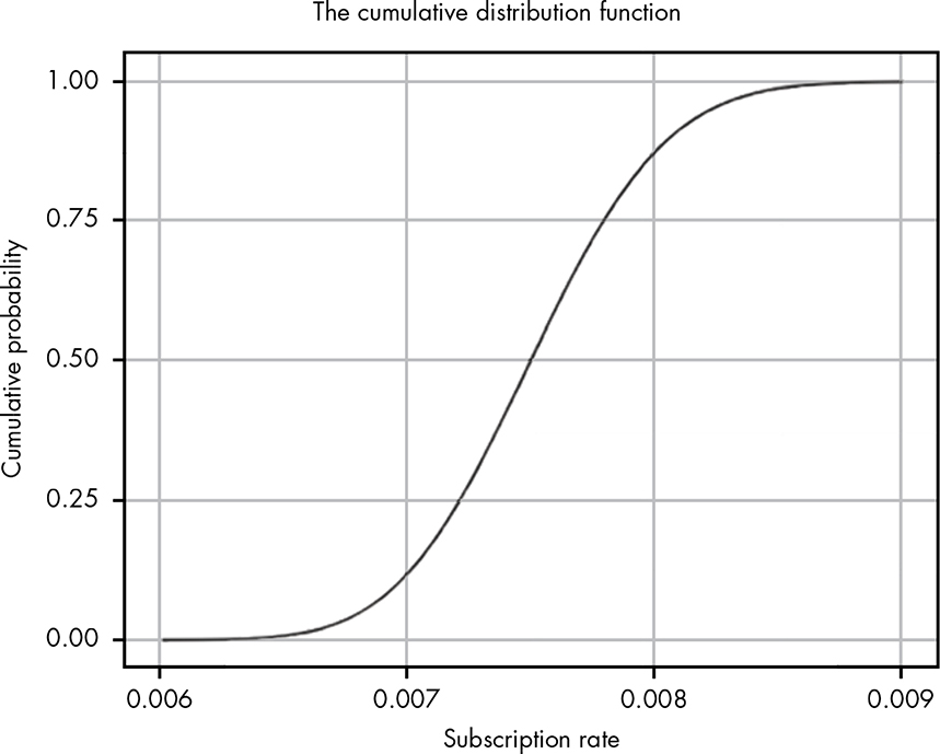
Figure 13-4: The CDF for our problem

Visualizing and Interpreting the CDF

The PDF is most useful visually for quickly estimating where the peak of a distribution is, and for getting a rough sense of the width (variance) and shape of a distribution. However, with the PDF it is very difficult to reason about the probability of various ranges visually. The CDF is a much better tool for this. For example, we can use the CDF in Figure 13-4 to visually reason about a much wider range of probabilistic estimates for our problem than we can using the PDF alone. Let’s go over a few visual examples of how we can use this amazing mathematical tool.

Finding the Median

The median is the point in the data at which half the values fall on one side and half on the other—it is the exact middle value of our data. In other words, the probability of a value being greater than the median and the probability of it being less than the median are both 0.5. The median is particularly useful for summarizing the data in cases where it contains extreme values.

Unlike the mean, computing the median can actually be pretty tricky. For small, discrete cases, it’s as simple as putting your observations in order and selecting the value in the middle. But for continuous distributions like our beta distribution, it’s a little more complicated.

Thankfully, we can easily spot the median on a visualization of the CDF. We can simply draw a line from the point where the cumulative probability is 0.5, meaning 50 percent of the values are below this point and 50 percent are above. As Figure 3-5 illustrates, the point where this line intersects the x-axis gives us our median!

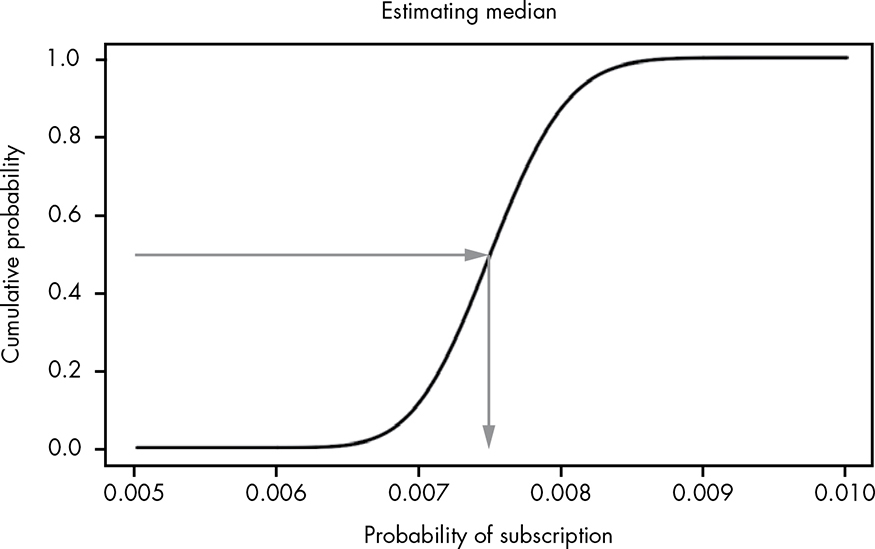
Figure 13-5: Estimating the median visually using the CDF

We can see that the median for our data is somewhere between 0.007 and 0.008 (this happens to be very close the mean of 0.0075, meaning the data isn’t particularly skewed).

Approximating Integrals Visually

When working with ranges of probabilities, we’ll often want to know the probability that the true value lies somewhere between some value y and some value x.

We can solve this kind of problem using integration, but even if R makes solving integrals easier, it’s very time-consuming to make sense of the data and to constantly rely on R to compute integrals. Since all we want is a rough estimate that the probability of a visitor subscribing to the blog falls within a particular range, we don’t need to use integration. The CDF makes it very easy to eyeball whether or not a certain range of values has a very high probability or a very low probability of occurring.

To estimate the probability that the conversion rate is between 0.0075 and 0.0085, we can trace lines from the x-axis at these points, then see where they meet up with the y-axis. The distance between the two points is the approximate integral, as shown in Figure 13-6.

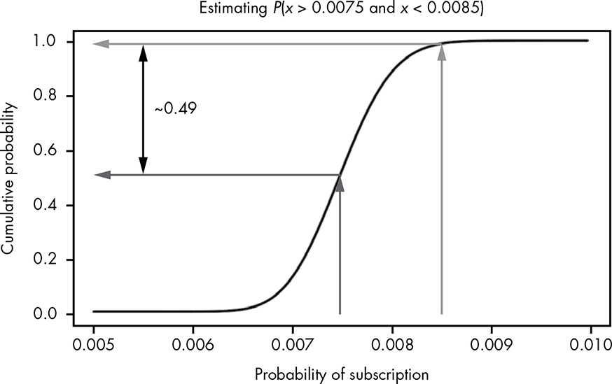
Figure 13-6: Visually performing integration using the CDF

We can see that on the y-axis these values range from roughly 0.5 to 0.99, meaning that there is approximately a 49 percent chance that our true conversion rate lies somewhere between these two values. The best part is we didn’t have to do any integration! This is, of course, because the CDF represents the integral from the minimum of our function to all possible values.

So, since nearly all of the probabilistic questions about a parameter estimate involve knowing the probability associated with certain ranges of beliefs, the CDF is often a far more useful visual tool than the PDF.

Estimating Confidence Intervals

Looking at the probability of ranges of values leads us to a very important concept in probability: the confidence interval. A confidence interval is a lower and upper bound of values, typically centered on the mean, describing a range of high probability, usually 95, 99, or 99.9 percent. When we say something like “The 95 percent confidence interval is from 12 to 20,” what we mean is that there is a 95 percent probability that our true measurement is somewhere between 12 and 20. Confidence intervals provide a good method of describing the range of possibilities when we’re dealing with uncertain information.

We can estimate confidence intervals using the CDF. Say we wanted to know the range that covers 80 percent of the possible values for the true conversion rate. We solve this problem by combining our previous approaches: we draw lines at the y-axis from 0.1 and 0.9 to cover 80 percent, and then simply see where on the x-axis these intersect with our CDF, as shown in Figure 13-7.

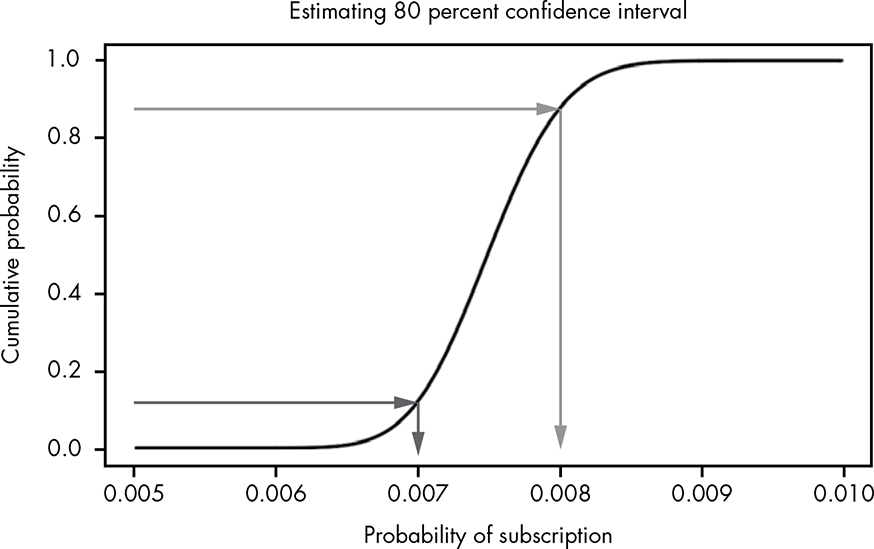
Figure 13-7: Estimating our confidence intervals visually using the CDF

As you can see, the x-axis is intersected at roughly 0.007 and 0.008, which means that there’s an 80 percent chance that our true conversion rate falls somewhere between these two values.

Using the CDF in R

Just as nearly all major PDFs have a function starting with d, like dnorm(), CDF functions start with p, such as pnorm(). In R, to calculate the probability that Beta(300,39700) is less than 0.0065, we can simply call pbeta() like this:

pbeta(0.0065,300,39700)
> 0.007978686

And to calculate the true probability that the conversion rate is greater than 0.0085, we can do the following:

pbeta(1,300,39700) - pbeta(0.0085,300,39700)
> 0.01248151

The great thing about CDFs is that it doesn’t matter if your distribution is discrete or continuous. If we wanted to determine the probability of getting three or fewer heads in five coin tosses, for example, we would use the CDF for the binomial distribution like this:

pbinom(3,5,0.5)
> 0.8125

The Quantile Function

You might have noticed that the median and confidence intervals we took visually with the CDF are not easy to do mathematically. With the visualizations, we simply drew lines from the y-axis and used those to find a point on the x-axis.

Mathematically, the CDF is like any other function in that it takes an x value, often representing the value we’re trying to estimate, and gives us a y value, which represents the cumulative probability. But there is no obvious way to do this in reverse; that is, we can’t give the same function a y to get an x. As an example, imagine we have a function that squares values. We know that square(3) = 9, but we need an entirely new function—the square root function—to know that the square root of 9 is 3.

However, reversing the function is exactly what we did in the previous section to estimate the median: we looked at the y-axis for 0.5, then traced it back to the x-axis. What we’ve done visually is compute the inverse of the CDF.

While computing the inverse of the CDF visually is easy for estimates, we need a separate mathematical function to compute it for exact values. The inverse of the CDF is an incredibly common and useful tool called the quantile function. To compute an exact value for our median and confidence interval, we need to use the quantile function for the beta distribution. Just like the CDF, the quantile function is often very tricky to derive and use mathematically, so instead we rely on software to do the hard work for us.

Visualizing and Understanding the Quantile Function

Because the quantile function is simply the inverse of the CDF, it just looks like the CDF rotated 90 degrees, as shown in Figure 13-8.

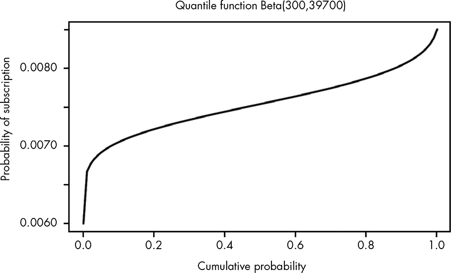
Figure 13-8: Visually, the quantile function is just a rotation of the CDF.

Whenever you hear phrases like:

“The top 10 percent of students . . .”

“The bottom 20 percent of earners earn less than . . .”

“The top quartile has notably better performance than . . .”

you’re talking about values that are found using the quantile function. To look up a quantile visually, just find the quantity you’re interested in on the x-axis and see where it meets the y-axis. The value on the y-axis is the value for that quantile. Keep in mind that if you’re talking about the “top 10 percent,” you really want the 0.9 quantile.

Calculating Quantiles in R

R also includes the function qnorm() for calculating quantiles. This function is very useful for quickly answering questions about what values are bounds of our probability distribution. For example, if we want to know the value that 99.9 percent of the distribution is less than, we can use qbeta() with the quantile we’re interested in calculating as the first argument, and the alpha and beta parameters of our beta distribution as the second and third arguments, like so:

qbeta(0.999,300,39700)
> 0.008903462

The result is 0.0089, meaning we can be 99.9 percent certain that the true conversion rate for our emails is less than 0.0089. We can then use the quantile function to quickly calculate exact values for confidence intervals for our estimates. To find the 95 percent confidence interval, we can find the values greater than the 2.5 percent lower quantile and the values lower than the 97.5 percent upper quantile, and the interval between them is the 95 percent confidence interval (the unaccounted region totals 5 percent of the probability density at both extremes). We can easily calculate these for our data with qbeta():

Our lower bound is qbeta(0.025,300,39700) = 0.0066781

Our upper bound is qbeta(0.975,300,39700) = 0.0083686

Now we can confidently say that we are 95 percent certain that the real conversion rate for blog visitors is somewhere between 0.67 percent and 0.84 percent.

We can, of course, increase or decrease these thresholds depending on how certain we want to be. Now that we have all of the tools of parameter estimation, we can easily pin down an exact range for the conversion rate. The great news is that we can also use this to predict ranges of values for future events.

Suppose an article on your blog goes viral and gets 100,000 visitors. Based on our calculations, we know that we should expect between 670 and 840 new email subscribers.

Wrapping Up

We’ve covered a lot of ground and touched on the interesting relationship between the probability density function (PDF), cumulative distribution function (CDF), and the quantile function. These tools form the basis of how we can estimate parameters and calculate our confidence in those estimations. That means we can not only make a good guess as to what an unknown value might be, but also determine confidence intervals that very strongly represent the possible values for a parameter.

Exercises

Try answering the following questions to see how well you understand the tools of parameter estimation. The solutions can be found in Appendix C.

1. Using the code example for plotting the PDF on page 127, plot the CDF and quantile functions.
2. Returning to the task of measuring snowfall from Chapter 10, say you have the following measurements (in inches) of snowfall:

   7.8, 9.4, 10.0, 7.9, 9.4, 7.0, 7.0, 7.1, 8.9, 7.4

   What is your 99.9 percent confidence interval for the true value of snowfall?

3. A child is going door to door selling candy bars. So far she has visited 30 houses and sold 10 candy bars. She will visit 40 more houses today. What is the 95 percent confidence interval for how many candy bars she will sell the rest of the day?