19
FROM HYPOTHESIS TESTING TO PARAMETER ESTIMATION

So far, we’ve used posterior odds to compare only two hypotheses. That’s fine for simple problems; even if we have three or four hypotheses, we can test them all by conducting multiple hypothesis tests, as we did in the previous chapter. But sometimes we want to search a really large space of possible hypotheses to explain our data. For example, you might want to guess how many jelly beans are in a jar, the height of a faraway building, or the exact number of minutes it will take for a flight to arrive. In all these cases, there are many, many possible hypotheses—too many to conduct hypothesis tests for all of them.

Luckily, there’s a technique for handling this scenario. In Chapter 15, we learned how to turn a parameter estimation problem into a hypothesis test. In this chapter, we’re going to do the opposite: by looking at a virtually continuous range of possible hypotheses, we can use the Bayes factor and posterior odds (a hypothesis test) as a form of parameter estimation! This approach allows us to evaluate more than just two hypotheses and provides us with a simple framework for estimating any parameter.

Is the Carnival Game Really Fair?

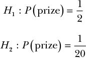
Suppose you’re at a carnival. While walking through the games, you notice someone arguing with a carnival attendant near a pool of little plastic ducks. Curious, you get closer and hear the player yelling, “This game is rigged! You said there was a 1 in 2 chance of getting a prize and I’ve picked up 20 ducks and only received one prize! It looks to me like the chance of getting a prize is only 1 in 20!”

Now that you have a strong understanding of probability, you decide to settle this argument yourself. You explain to the attendant and the angry customer that if you observe some more games that day, you’ll be able to use the Bayes factor to determine who’s right. You decide to break up the results into two hypotheses: H₁, which represents the attendant’s claim that the probability of a prize is 1/2, and H₂, the angry customer’s claim that the probability of a prize is just 1/20:

The attendant argues that because he didn’t watch the customer pick up ducks, he doesn’t think you should use his reported data, since no one else can verify it. This seems fair to you. You decide to watch the next 100 games and use that as your data instead. After the customer has picked up 100 ducks, you observe that 24 of them came with prizes.

Now, on to the Bayes factor! Since we don’t have a strong opinion about the claim from either the customer or the attendant, we won’t worry about the prior odds or calculating our full posterior odds yet.

To get our Bayes factor, we need to compute P(D | H) for each hypothesis:

P(D | H₁) = (0.5)²⁴ × (1 – 0.5)⁷⁶

P(D | H₂) = (0.05)²⁴ × (1 – 0.05)⁷⁶

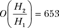
Now, individually, both of these probabilities are quite small, but all we care about is the ratio. We’ll look at our ratio in terms of H₂/H₁ so that our result will tell us how many times better the customer’s hypothesis explains the data than the attendant’s:

Our Bayes factor tells us that H₁, the attendant’s hypothesis, explains the data 653 times as well as H₂, which means that the attendant’s hypothesis (that the probability of getting a prize when picking up a duck is 0.5) is the more likely one.

This should immediately seem strange. Clearly, the probability of getting only 24 prizes out of a total of 100 ducks seems really unlikely if the true probability of a prize is 0.5. We can use R’s pbinom() function (introduced in Chapter 13) to calculate the binomial distribution, which will tell us the probability of seeing 24 or fewer prizes, assuming that the probability of getting a prize is really 0.5:

> pbinom(24,100,0.5)
9.050013e-08

As you can see, the probability of getting 24 or fewer prizes if the true probability of a prize is 0.5 is extremely low; expanding it out to the full decimal values, we get a probability of 0.00000009050013! Something is definitely up with H₁. Even though we don’t believe the attendant’s hypothesis, it still explains the data much better than the customer’s.

So what’s missing? In the past, we’ve often found that the prior probability usually matters a lot when the Bayes factor alone doesn’t give us an answer that makes sense. But as we saw in Chapter 18, there are cases in which the prior isn’t the root cause of our problem. In this case, using the following equation seems reasonable, since we don’t have a strong opinion either way:

But maybe the problem here is that you have a preexisting mistrust in carnival games. Because the result of the Bayes factor favors the attendant’s hypothesis so strongly, we’d need our prior odds to be at least 653 to get a posterior odds that favors the customer’s hypothesis:

That’s a really deep distrust of the fairness of the game! There must be some problem here other than the prior.

Considering Multiple Hypotheses

One obvious problem is that, while it seems intuitively clear that the attendant is wrong in his hypothesis, the customer’s alternative hypothesis is just too extreme to be right, either, so we have two wrong hypotheses. What if the customer thought the probability of winning was 0.2, rather than 0.05? We’ll call this hypothesis H₃. Testing H₃ against the attendant’s hypothesis radically changes the results of our likelihood ratio:

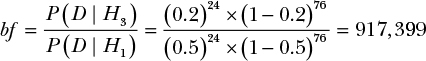
Here we see that H₃ explains the data wildly better than H₁. With a Bayes factor of 917,399, we can be certain that H₁ is far from the best hypothesis for explaining the data we’ve observed, because H₃ blows it out of the water. The trouble we had in our first hypothesis test was that the customer’s belief was a far worse description of the event than the attendant’s belief. As we can see, though, that doesn’t mean the attendant was right. When we came up with an alternative hypothesis, we saw that it was a much better guess than either the attendant’s or the customer’s.

Of course, we haven’t really solved our problem. What if there’s an even better hypothesis out there?

Searching for More Hypotheses with R

We want a more general solution that searches all of our possible hypotheses and picks out the best one. To do this, we can use R’s seq() function to create a sequence of hypotheses we want to compare to our H₁.

We’ll consider every increment of 0.01 between 0 and 1 as a possible hypothesis. That means we’ll consider 0.01, 0.02, 0.03, and so on. We’ll call 0.01—the amount we’re increasing each hypothesis by—dx (a common notation from calculus representing the “smallest change”) and use it to define a hypotheses variable, which represents all of the possible hypotheses we want to consider. Here we use R’s seq() function to generate a range of values for each hypothesis between 0 and 1 by incrementing the values by our dx:

dx <- 0.01
hypotheses <- seq(0,1,by=dx)

Next, we need a function that can calculate our likelihood ratio for any two hypotheses. Our bayes.factor() function will take two arguments: h_top, which is the probability of getting a prize for the hypothesis on the top (the numerator) and h_bottom, which is the hypothesis we’re competing against (the attendant’s hypothesis). We set this up like so:

bayes.factor <- function(h_top,h_bottom){
  ((h_top)^24*(1-h_top)^76)/((h_bottom)^24*(1-h_bottom)^76)
}

Finally, we compute the likelihood ratio for all of these possible hypotheses:

bfs <- bayes.factor(hypotheses,0.5)

Then, we use R’s base plotting functionality to see what these likelihood ratios look like:

plot(hypotheses,bfs, type='l')

Figure 19-1 shows the resulting plot.

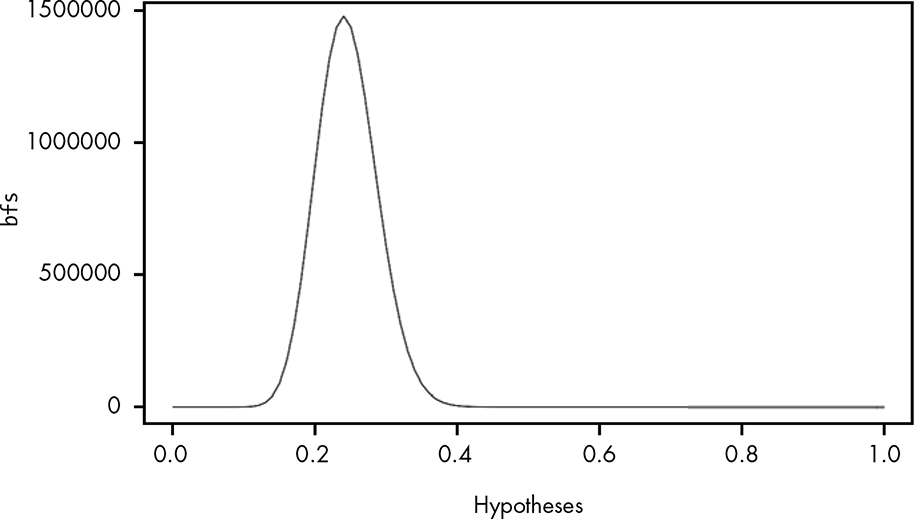
Figure 19-1: Plotting the Bayes factor for each of our hypotheses

Now we can see a clear distribution of different explanations for the data we’ve observed. Using R, we can look at a wide range of possible hypotheses, where each point in our line represents the Bayes factor for the corresponding hypothesis on the x-axis.

We can also see how high the largest Bayes factor is by using the max() function with our vector of bfs:

> max(bfs)
1.47877610^{6}

Then we can check which hypothesis corresponds to the highest likelihood ratio, telling us which hypothesis we should believe in the most. To do this, enter:

> hypotheses[which.max(bfs)]
0.24

Now we know that a probability of 0.24 is our best guess, since this hypothesis produces the highest likelihood ratio when compared with the attendant’s. In Chapter 10, you learned that using the mean or expectation of our data is often a good way to come up with a parameter estimate. Here we’ve simply chosen the hypothesis that individually explains the data the best, because we don’t currently have a way to weigh our estimates by their probability of occurring.

Adding Priors to Our Likelihood Ratios

Now suppose you present your findings to the customer and the attendant. Both agree that your findings are pretty convincing, but then another person walks up to you and says, “I used to make games like these, and I can tell you that for some strange industry reason, the people who design these duck games never put the prize rate between 0.2 and 0.3. I’d bet you the odds are 1,000 to 1 that the real prize rate is not in this range. Other than that, I have no clue.”

Now we have some prior odds that we’d like to use. Since the former game maker has given us some solid odds about his prior beliefs in the probability of getting a prize, we can try to multiply this by our current list of Bayes factors and compute the posterior odds. To do this, we create a list of prior odds ratios for every hypothesis we have. As the former game maker told us, the prior odds ratio for all probabilities between 0.2 and 0.3 should be 1/1,000. Since the maker has no opinion about other hypotheses, the odds ratio for these will just be 1. We can use a simple ifelse statement, using our vector of hypotheses, to create a vector of our odds ratios:

priors <- ifelse(hypotheses >= 0.2 & hypotheses <= 0.3, 1/1000,1)

Then we can once again use plot() to display this distribution of priors:

plot(hypotheses,priors,type='l')

Figure 19-2 shows our distribution of prior odds.

Because R is a vector-based language (for more information on this, see Appendix A), we can simply multiply our priors by our bfs and get a new vector of posteriors representing our Bayes factors:

posteriors <- priors*bfs

Finally, we can plot a chart of the posterior odds of each of our many hypotheses:

plot(hypotheses,posteriors,type='l')

Figure 19-3 shows the plot.

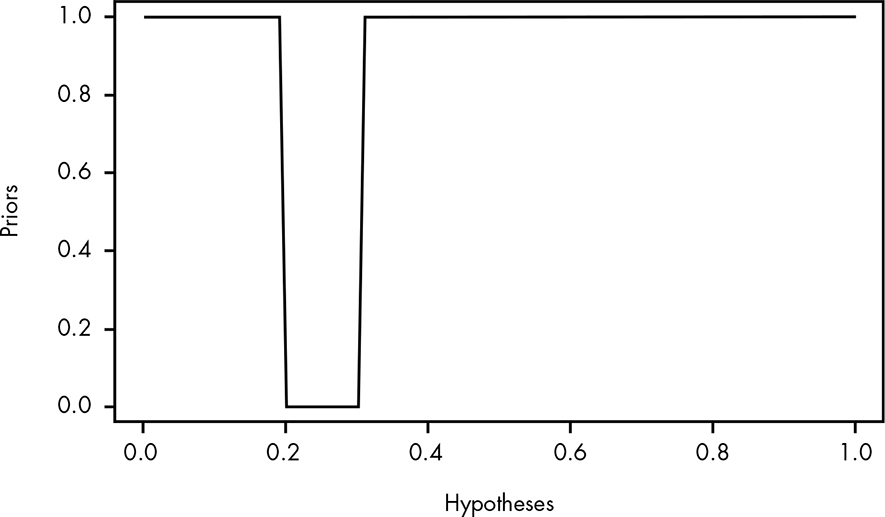
Figure 19-2: Visualizing our prior odds ratios

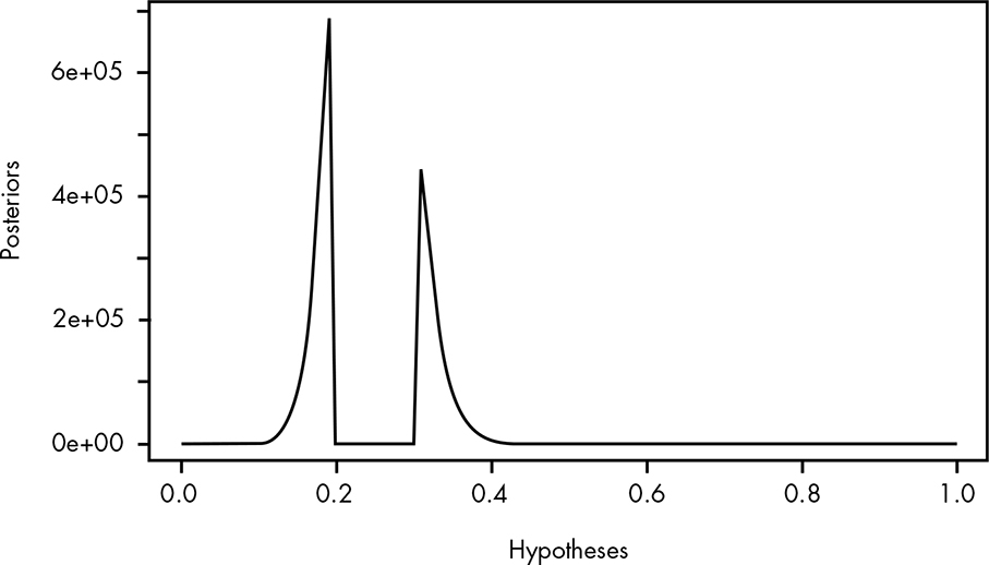
Figure 19-3: Plotting our distribution of Bayes factors

As we can see, we get a very strange distribution of possible beliefs. We have reasonable confidence in the values between 0.15 and 0.2 and between 0.3 and 0.35, but find the range between 0.2 and 0.3 to be extremely unlikely. But this distribution is an honest representation of the strength of belief in each hypothesis, given what we’ve learned about the duck game manufacturing process.

While this visualization is helpful, we really want to be able to treat this data like a true probability distribution. That way, we can ask questions about how much we believe in ranges of possible hypotheses and calculate the expectation of our distribution to get a single estimate for what we believe the hypothesis to be.

Building a Probability Distribution

A true probability distribution is one where the sum of all possible beliefs equals 1. Having a probability distribution would allow us to calculate the expectation (or mean) of our data to make a better estimate about the true rate of getting a prize. It would also allow us to easily sum ranges of values so we could come up with confidence intervals and other similar estimates.

The problem is that if we add up all the posterior odds for our hypotheses, they don’t equal 1, as shown in this calculation:

> sum(posteriors)
3.140687510^{6}

This means we need to normalize our posterior odds so that they do sum to 1. To do so, we simply divide each value in our posteriors vector by the sum of all the values:

p.posteriors <- posteriors/sum(posteriors)

Now we can see that our p.posteriors values add up to 1:

> sum(p.posteriors)
1

Finally, let’s plot our new p.posteriors:

plot(hypotheses,p.posteriors,type='l')

Figure 19-4 shows the plot.

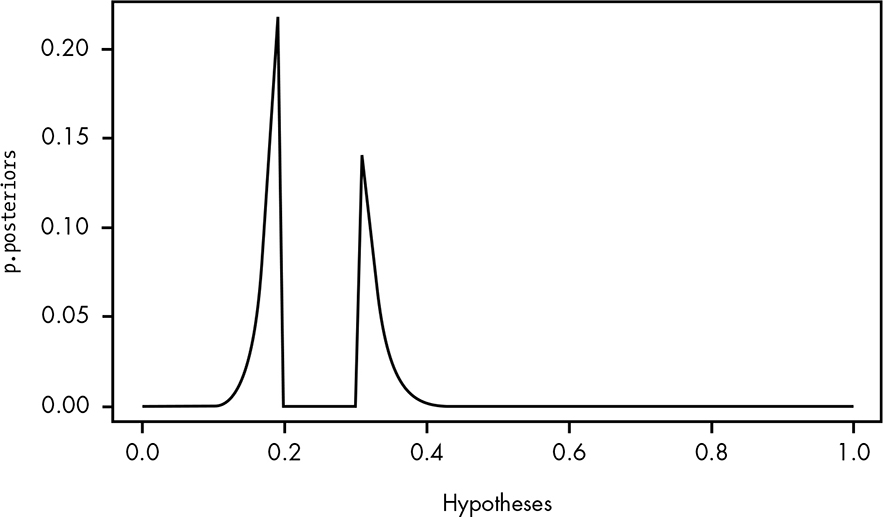
Figure 19-4: Our normalized posterior odds (note the scale on the y-axis)

We can also use our p.posteriors to answer some common questions we might have about our data. For example, we can now calculate the probability that the true rate of getting a prize is less than what the attendant claims. We just add up all the probabilities for values less than 0.5:

sum(p.posteriors[which(hypotheses < 0.5)])
> 0.9999995

As we can see, the probability that the prize rate is lower than the attendant’s hypothesis is nearly 1. That is, we can be almost certain that the attendant is overstating the true prize rate.

We can also calculate the expectation of our distribution and use this result as our estimate for the true probability. Recall that the expectation is just the sum of the estimates weighted by their value:

> sum(p.posteriors*hypotheses)
0.2402704

Of course, we can see our distribution is a bit atypical, with a big gap in the middle, so we might want to simply choose the most likely estimate, as follows:

> hypotheses[which.max(p.posteriors)]
0.19

Now we’ve used the Bayes factor to come up with a range of probabilistic estimates for the true possible rate of winning a prize in the duck game. This means that we’ve used the Bayes factor as a form of parameter estimation!

From the Bayes Factor to Parameter Estimation

Let’s take a moment to look at our likelihood ratios alone again. When we weren’t using a prior probability for any of the hypotheses, you might have felt that we already had a perfectly good approach to solving this problem without needing the Bayes factor. We observed 24 ducks with prizes and 76 ducks without prizes. Couldn’t we just use our good old beta distribution to solve this problem? As we’ve discussed many times since Chapter 5, if we want to estimate the rate of some event, we can always use the beta distribution. Figure 19-5 shows a plot of a beta distribution with an alpha of 24 and a beta of 76.

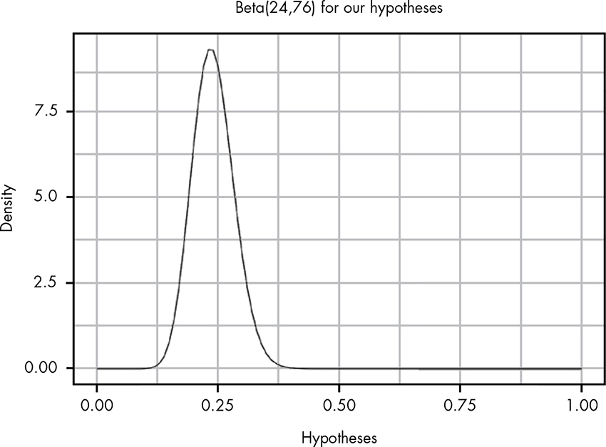
Figure 19-5: The beta distribution with an alpha of 24 and a beta of 76

Except for the scale of the y-axis, the plot looks nearly identical to the original plot of our likelihood ratios! In fact, if we do a few simple tricks, we can get these two plots to line up perfectly. If we scale our beta distribution by the size of our dx and normalize our bfs, we can see that these two distributions get quite close (Figure 19-6).

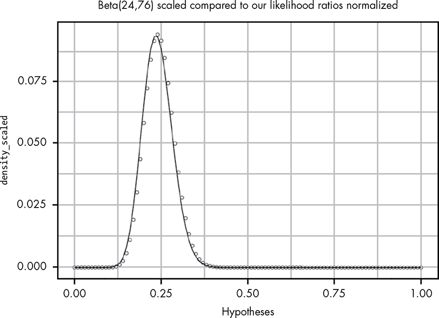
Figure 19-6: Our initial distribution of likelihood ratios maps pretty closely to Beta(24,76).

There seems to be only a slight difference now. We can fix it by using the weakest prior that indicates that getting a prize and not getting a prize are equally likely—that is, by adding 1 to both the alpha and beta parameters, as shown in Figure 19-7.

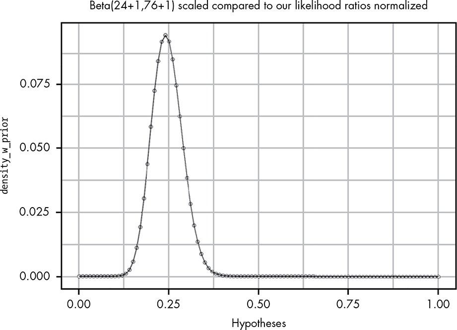
Figure 19-7: Our likelihood ratios map perfectly to a Beta(24+1,76+1) distribution.

Now we can see that the two distributions are perfectly aligned. Chapter 5 mentioned that the beta distribution was difficult to derive from our basic rules of probability. However, by using the Bayes factor, we’ve been able to empirically re-create a modified version of it that assumes a prior of Beta(1,1). And we did it without any fancy mathematics! All we had to do was:

1. Define the probability of the evidence given a hypothesis.
2. Consider all possible hypotheses.
3. Normalize these values to create a probability distribution.

Every time we’ve used the beta distribution in this book, we’ve used a beta-distributed prior. This made the math easier, since we can arrive at the posterior by combining the alpha and beta parameters from the likelihood and prior beta distributions. In other words:

Beta(α_posterior, β_posterior) = Beta(α_prior + α_likelihood, β_prior + β_likelihood)

However, by building our distribution from the Bayes factor, we were able to easily use a unique prior distribution. Not only is the Bayes factor a great tool for setting up hypothesis tests, but, as it turns out, it’s also all we need to create any probability distribution we might want to use to solve our problem, whether that’s hypothesis testing or parameter estimation. We just need to be able to define the basic comparison between two hypotheses, and we’re on our way.

When we built our A/B test in Chapter 15, we figured out how to reduce many hypothesis tests to a parameter estimation problem. Now you’ve seen how the most common form of hypothesis testing can also be used to perform parameter estimation. Given these two related insights, there is virtually no limit to the type of probability problems we can solve using only the most basic rules of probability.

Wrapping Up

Now that you’ve finished your journey into Bayesian statistics, you can appreciate the true beauty of what you’ve been learning. From the basic rules of probability, we can derive Bayes’ theorem, which lets us convert evidence into a statement expressing the strength of our beliefs. From Bayes’ theorem, we can derive the Bayes factor, a tool for comparing how well two hypotheses explain the data we’ve observed. By iterating through possible hypotheses and normalizing the results, we can use the Bayes factor to create a parameter estimate for an unknown value. This, in turn, allows us to perform countless other hypothesis tests by comparing our estimates. And all we need to do to unlock all this power is use the basic rules of probability to define our likelihood, P(D | H)!

Exercises

Try answering the following questions to see how well you understand using the Bayes factor and posterior odds to do parameter estimation. The solutions can be found in Appendix C.

1. Our Bayes factor assumed that we were looking at H₁: P(prize) = 0.5. This allowed us to derive a version of the beta distribution with an alpha of 1 and a beta of 1. Would it matter if we chose a different probability for H₁? Assume H₁: P(prize) = 0.24, then see if the resulting distribution, once normalized to sum to 1, is any different than the original hypothesis.
2. Write a prior for the distribution in which each hypothesis is 1.05 times more likely than the previous hypothesis (assume our dx remains the same).
3. Suppose you observed another duck game that included 34 ducks with prizes and 66 ducks without prizes. How would you set up a test to answer “What is the probability that you have a better chance of winning a prize in this game than in the game we used in our example?” Implementing this requires a bit more sophistication than the R used in this book, but see if you can learn this on your own to kick off your adventures in more advanced Bayesian statistics!