
2 Linear and nonlinear properties (!) of straight lines
Q: When is a straight line not a straight line? A: When it has been bent!
Now we might well be thinking ‘Why would we want to do that as we have already intimated that straight lines are easier to extrapolate or project than curves?’ However, in the case of sequential linear relationships, we don’t have to bend straight lines because they already possess the property that their Cumulative Values always form a Quadratic Function (i.e. a Polynomial of Order 2) – a distinctly curved line. Furthermore, the Quadratic will have coefficients or parameters that are simple functions of the slope and intercept of the straight line.
Before we delve into this perhaps lesser known property, let’s remind ourselves of some of the basic properties that are relevant to all straight lines.
2.1 Basic linear properties
The most significant property of a straight line is its constant monotonicity (see Volume II Chapter 5), i.e. its unwavering progression in one direction. Any position on the straight line can be determined by two parameters or constants (the slope and the intercept) and a single variable. Conversely, any two points on a straight line are sufficient to determine the slope and the intercept.
For the Formula-phobes: Two points define a straight line
Consider any two points on a graph. We can only draw one straight line through the two points. The two points uniquely define the slope (or gradient) and the intercept (the value on the vertical axis corresponding with the zero value on the horizontal axis.


The left-hand example has a positive or increasing slope, whereas the right-hand example has a negative or decreasing slope. Although not shown here, we could re-draw the horizontal axis higher up so that the intercept was negative in both cases.
For the Formula-philes: Two points define a straight line


As we selected the two points at random from the straight line, we can substitute either or both of them with any other point(s) on the line and the property remains intact.
If we have three or more data points formed by two highly (but not perfectly) correlated variables (Volume II Chapter 5) then we can draw a range of different straight lines through the points with varying errors where the line fails to pass through one or more points. However, the range of potential lines will be fairly narrow in terms of the potential values of slope and intercept, as illustrated on the left of Figure 2.1. The range of potential lines will be narrow if we are going to enter into the spirit and intent of making a reasonable effort of passing through the area occupied by the data points.
Where we have three or more such points that are poorly correlated, the range of straight lines we can draw through the points is wider, and the individual errors or scatter around the lines are greater, illustrated on the right of Figure 2.1. Both these cases are part of the ‘less than perfect world’ with which the estimator has to contend.

Figure 2.1 Examples of Lines of Imperfect Fit
In Chapter 4 we will be discussing how we can define what we mean by the ‘Best Fit straight line’ through some data, but in essence when we do this we are implying that the true underlying relationship approximates to a perfect straight line, and that any disparity between the straight line and the actual data, is an imperfection in the actual. Well, that is a bit of an overstatement, but we do tend to rely on the line first and then look at the potential scatter around the line as a bit of an afterthought, don’t we?
2.1.1 Inter-relation between slope and intercept
Taking the general equation of a straight line, we can easily show that for both positive and negative slopes or gradients, any straight line can be expressed as a function of its intercepts with the horizontal (x) and vertical (y) axes.
Consider the diagrams in Figure 2.2. Note that with the left-hand pair of graphs that the horizontal intercept d is negative whereas for the right-hand pair it is positive. Also, in the diagonal top-left to bottom-right, the vertical intercept c is positive, whereas on the cross-diagonal it is negative.
This also shows us that for any straight line with a positive slope (i.e. top pair of graphs), then one (but not both) of the intercepts is negative, and the other is positive . . . or both are zero. For a straight line which has a negative slope (i.e. the bottom pair of graphs in Figure 2.2), then both intercepts are either positive or negative together, or again, both are zero.
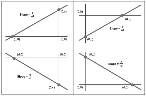
Figure 2.2 Slope as a Function of the Intercepts
For the Formula-philes: Straight lines as functions of their intercepts
Let (d, 0) and (0, c) be the intercepts of a straight line with the x and y axes respectively:

This is an important property when we come to Lines of Best Fit in the Chapter 4 as it illustrates that for any fixed horizontal intercept, the vertical intercept is either perfectly positively or negatively correlated with the slope of the line:
- If the horizontal intercept is negative, then the vertical intercept and the slope are positively correlated (as we increase one, the other increases in direct proportion)
- If the horizontal intercept is positive, then the vertical intercept and the slope are negatively correlated (as we increase one, the other decreases in direct proportion)
2.1.2 The difference between two straight lines is a straight line
It is sometimes a helpful property of straight lines that the difference between any two straight lines is also a straight line. Clearly the two lines should be measuring the things that can be compared such as the planned spend over time and the actual spend over the same time period. However, it might not make sense to subtract the linear trend in the total number of apples being eaten each month from the trend in the total number of oranges being eaten. (This would clearly be the classic mistake of comparing apples with oranges – unless we’re doing a fruit popularity contest, of course!)
This difference property allows us to compare linear variance trends. Note: Whilst the property is inviolable for perfect straight lines (i.e. it is always true), and can be read across to ‘real’ data which depict linear trends, there may be some difference in the results between the trend through the differences, and the difference between the two original trendlines. We can get this sometimes due to smoothing or worsening of the data scatter attributable to the difference.
For the Formula-phobes: Difference between two straight lines is a straight line
Draw any two lines on a piece of graph paper (or the electronic equivalent). It doesn’t matter if they cross.
Pick a point at random on the horizontal x-axis and measure the vertical difference between the two lines for that point. Repeat the exercise for a number of other points. Plot these differences to get another straight line, making sure that you have taken account of the change in sign if the lines have crossed
The reason this will always work is that we are measuring the rate at which the difference changes, which is the difference in the slopes of the two original lines.

For the Formula-philes: Difference between two straight lines is a straight line
Consider two straight lines:
2.2 The Cumulative Value (nonlinear) property of a linear sequence
As estimators, we will come across two types of straight line relationships (and I’m not talking about upward and downward sloping functions.) We will find that there are discrete functions in which the independent x-variable can only take specific values such as integers, and there are continuous functions which can take any value.
Even then we can sub-divide these relationships into two further types:
- There are those straight lines which represent the relationship between two correlated variables (including all analogical comparisons.) An example might be the cost of component testing in relation to the component’s weight.
- Then there are those straight lines which are parametric sequences of data, and for which we might want to consider exploring the cumulative value of the sequence. For example, the cost of successive units produced.
In the case of the former, it would make no sense to aggregate the data. This section is devoted to exploring the second type, sequential linear relationships that can be aggregated across the sequence.
2.2.1 The Cumulative Value of a Discrete Linear Function
Consider the case where the independent variable (depicted normally by the horizontal x-axis) of a linear function can only take discrete integer values, such as a build sequence number, or some time counter like the number of weeks or months from a project start:
- The Cumulative Average of that perfect straight line is another perfect straight line of half the slope.
- A corollary of this is that the Cumulative Value of that straight line forms a perfect quadratic equation (i.e. a polynomial of order 2) that passes through the origin
For the Formula-philes: Cumulative Value of a Discrete Linear Function
Consider a straight line with slope m and intercept c, in which the independent variable x represents the sequence of consecutive positive integers xi from 1 to n:


For the Formula-phobes: The Cumulative Average of a straight line is a straight line

The slope of a line is defined as the vertical movement divided by the horizontal movement (just like on a road). As shown in the diagram, the average of first two points is halfway between them but is plotted at x = 2. The average of the first three is halfway between them, and is plotted at x = 3; and so on, resulting in a line of half the slope of the original.
Both lines have been projected back to the vertical axis to show the impact on the theoretical Cumulative Average Intercept. (It’s theoretical because we can’t have a Cumulative Average based on zero quantity!)
Now that’s what I call mathe-magic!
However, some of us quite righty, might be asking ourselves, ‘Why this is useful? When would we ever use this property?’ However, this is not just some academic property, it does have practical applications. For instance:
- The independent variable may be a build sequence number, or a time period, which may be a good indicator of improvement (or degradation) in something that we are trying to estimate, but our detailed records are incomplete for whatever reason (if only we lived in that perfect world, estimating would be so much easier).
- Some data we may have been collecting in a natural sequence, may be quite erratic with peaks and troughs, but a Moving Average or Cumulative Average (see Chapter 3) may indicate an underlying linear trend.
Table 2.1 illustrates both these scenarios. In this example we have started to collect the detailed weekly data on the number of sales enquiries received during an ongoing marketing campaign somewhat later than we should have done. (Yes, this was very remiss of us, and with the benefit of hindsight we should have collected it earlier, but hey, this example is meant to represent the failings of real life!) However, all is not lost as we do have the cumulative data from the start of the campaign available to us.
The end column in the example, which calculates the Cumulative Average Number of Enquiries per Week, shows that there is an incremental increase week on week.
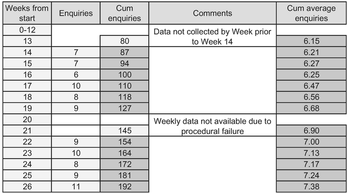
Table 2.1 Example – Enquiries Received Following Marketing Campaign
Figure 2.3 plots the Cumulative Number of Enquiries received and we can fit a Polynomial Trendline (order 2) using Microsoft Excel’s Chart utility and project it back to the start of the marketing campaign. In this case we appear to have a very good fit, indicated by the Coefficient of Determination R2 being so close to 1.
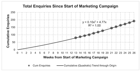
Figure 2.3 Example – Cumulative Enquiries Received Following Marketing Campaign
Note: Cumulative values are inherently much smoother than the unit data from which they are calculated. In this case it appears to be a near perfect quadratic relationship. However, if we were to expand the Coefficient of Determination to 3 decimal places, we would show that R2 ≠ 1.
The underlying linear trend that gives rise to this Cumulative Quadratic Function can be determined from the coefficients of the quadratic equation:
- The slope of this straight line is double the coefficient of the x2 term in the quadratic; in this case, the slope is 0.20, i.e. 2 times 0.10
- The intercept of the straight line is the difference between the quadratic coefficients of the x and x2 terms; in this case, 4.77 minus 0.10, or 4.67
Alternatively, we could have simply run a trendline through the weekly data or even the Cumulative Average data, as shown in Figure 2.4. If we use our rule that the Cumulative Average of a straight line is another straight line of half the slope, then based on the trendline through the Cumulative Average, the underlying linear function can be determined as follows:
- The Cumulative Average trendline slope is 0.10, so the underlying data has a slope of 0.2
- The intercept of the underlying straight line is the difference between the intercept and slope of the Cumulative Average. In this case the underlying intercept is 4.79 minus 0.1, or 4.69. Note that this is slightly different to the Cumulative Technique used above due to difference in the scatter around each line (e.g. one term is squared.)

Figure 2.4 Example – Weekly Enquiries Received Following Marketing Campaign
These values are very compatible with the results from the Cumulative Quadratic Model (not surprisingly as they use the same data), but they are distinctly different to the simple trendline through the raw data, which gives us a steeper slope of 0.24, and smaller intercept of 3.75 in this instance. Now, we may be alarmed by this as they are based on the same data, whereas in reality, we have two more data points for the Cumulative and Cumulative Average Technique (Week 13 and 21 data can be derived by subtracting the weekly data from the cumulative for Weeks 14 and 22). However, notwithstanding that, if we were to remove these additional points (at x = 13 and x = 21) we would still get a different answer because of the degree and manner of the scatter in the raw data.
So, which should we use? We do have a choice, of course, but we may want to take account of the fact that in this case the Coefficient of Determination for the simple trendline through the raw data is not very encouraging (less than 0.5 – see Volume II, Chapter 5.) We should always go back to one of the basic premises of estimating – no single technique is foolproof. So we could use both in order to establish a range estimate.
Now, let’s consider other, perhaps more basic uses of the Cumulative Quadratic property. Suppose we wanted to project how many enquiries we would have received after twelve months, and how many a week we could expect to receive if the campaign continued to have the success it appears to be having now?
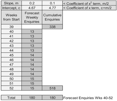
Table 2.2 Example – Using the Quadratic Formula to Forecast the Cumulative Value
A by-product of this Cumulative Quadratic property is that we can very quickly get a cumulative forecast for a future batch or for a period of time:
- We can extrapolate our linear trend to cover the range of values in which we are interested. We can then calculate the value of every valid unit, and add them up (and yes, it is easy to do that in spreadsheets like Microsoft Excel)
- Alternatively, we can calculate the cumulative value of our end-point using our quadratic formula and deduct the cumulative value immediately prior to our start-point, again using our quadratic formula
Table 2.2 illustrates both ways using our marketing campaign example.
Note: Due to rounding errors with discrete data, we can sometimes get slightly different answers between these two techniques.
2.2.2 The Cumulative Value of a Continuous Linear Function
Let’s turn our attention to straight lines which are Continuous Linear Functions in which the input x-variable can take any value, not just integers. Examples of this might include the equivalent unit build quantity which includes incomplete units e.g. 2.25 units (rather than completed units which would be integer values only.)
If we are taking equivalent units into account rather than just completed units, then we need to ensure than the two are compatible, i.e. they both give the same Cumulative Value in a perfect world. (In reality, they will give comparable results, but we’ll come back to that later in this section.)
Let’s revisit the Cumulative of the discrete linear relationship and look at it from a different perspective – as the sum of a number of areas.
Each point on the discrete straight line is the mid-point of the two points, half a unit to its left and right. If we multiply this by one, we get the area of the trapezium, Ti. We can repeat this process for each successive integer value representing points on the straight line, giving trapezia T1 to Tn inclusively, as illustrated in Figure 2.5.
The area of a trapezium is the average length of the two parallel sides multiplied by their distance apart.
Here, we are using the British definition of trapezium with two sides parallel, which is what Americans call a trapezoid, which in British usage is a quadrilateral with no parallel sides. In other words, American definitions are crossed over! What was it that George Bernard Shaw commented?
A word (or two) from the wise?
"England and America are two countries separated by a common language."
George Bernard Shaw Irish Playwright (1856-1950)
The sum of all these British trapezia can be added together to get one large trapezium (Figure 2.6) that equals the sum of the consecutive discrete values on a straight line. This trapezium is bounded by the values x = 0.5, x = n+0.5, the x-axis and the straight line. If we slide the trapezium representing the sum of discrete values to the left by half a unit, then we get a trapezium of equal area that is the integral of the Continuous Function (see Figure 2.7). In this case the trapezium is bounded by x = 0 and x = n.
In Volume II Chapter 4 we may have seen that the integral of a function gave the area under the curve and that this was the cumulative probability. We can use the area under this offset graph to represent the cumulative value of a Continuous Linear Function rather than the ‘true’ Discrete Linear Function. (Actually, we can use the area under the discrete version but as we have already shown that to get the correct value we have to start at 0.5 and end at n+0.5 rather than 0 through to n. It just doesn’t feel right, does it?)
‘And the point of all this?’ some of us may be asking. As a consequence, we can use the same quadratic equation to simulate the Cumulative Value of a straight line regardless of whether it is a discrete or Continuous Linear Function. The Continuous Function allows us to emulate the equivalent number of units built rather than just completed units, i.e. to include work-in-progress.
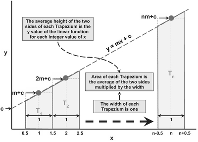
Figure 2.5 Straight Line Discrete Values Expressed as Trapezial Areas Under the Line

Figure 2.6 Cumulative of a Discrete Value Straight Line as a Trapezial Area Under the Line
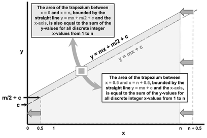
Figure 2.7 Equating Cumulative Values for Discrete and Continuous Straight Lines
Don’t you just love it when everything comes together logically like a well laid plan? No? There’s just no pleasing some people!
For the Formula-philes: Cumulative Value of a Continuous Linear Function
Consider a straight line with slope m and intercept , in which the

Figure 2.8 and Table 2.3 illustrate the equivalence of the single quadratic model for both cases. For clarity, we are demonstrating the results for a perfect straight line unit budget which assumes that the man-hours required to complete a recurring task reduce by 10 hours on each successive unit completed, with an intercept value of 210 hours, and that these hours will be expended in a fixed percentage pattern over a constant three-week build cycle.
The quadratic model, therefore, assumes a coefficient of -5 for the square of the build number term (half the slope), and 205 for the coefficient applied to the build number term (i.e. linear intercept plus half the slope):
The lower of the two graphs shows the Cumulative Budget Profile using this quadratic model, against which we have plotted the data created manually from the table, using both the Cumulative Budget for completed units, and the Cumulative Equivalent Build Units completed at the end of each week.
Note: This is not quite the perfect fit it appears, but in the context of an estimate, the difference can be considered to be insignificant (i.e. we are seeking accuracy not precision after all.)
Caveat augur
When we examine continuous sequential data in graphical or tabular form, the interval between successive observations in the sequence may not be regular. When this is the case the value we are measuring or estimating will vary depending on how much of the sequential data has moved on cumulatively. As a consequence, it is unlikely that the data we observe will appear to be linear – even if the underlying relationship is perfectly linear, and the cumulative data is quadratic. This is just a reporting paradox.
If the cumulative sequential data is a fixed interval, then we will see the underlying straight line, or at least a close approximation.
This concept may not be intuitive. However, we can see it in action in the current example. In Figure 2.9 we have plotted the planned budget for each week against the planned equivalent units to be completed – clearly not a linear plot.
However, if we were to re-profile the data (same cumulative hours) so that each week we were to complete the same number of equivalent units, we would get the results in Table 2.4 and Figure 2.10:
We will get the same reporting paradox with discrete sequential linear data also. If we review data ad hoc rather than at fixed sequential intervals, then we may not observe the underlying linear relationship.
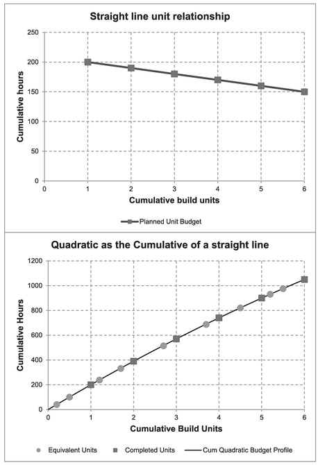
Figure 2.8 Example – Using the Quadratic Formula to Forecast the Cumulative Value

Table 2.3 Example – Using the Quadratic Formula and Equivalent Units to Forecast the Cumulative Value
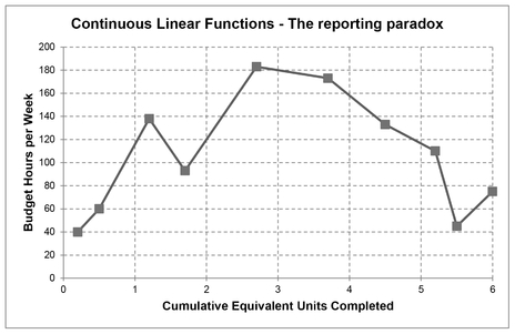
Figure 2.9 Continuous Linear Functions – The Reporting Paradox
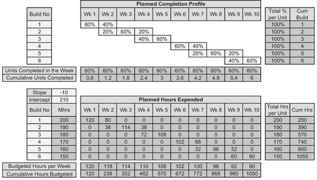
Table 2.4 Example Revisited with Steady State Equivalent Unit Completions

Figure 2.10 Continuous Linear Functions – The Reporting Paradox Revisited
2.2.3 Exploiting the Quadratic Cumulative Value of a straight line
There are two obvious ways in which we can exploit this Quadratic Cumulative Value property. If we believe (or better still have evidence) that there is an underlying linear trend in some sequential data, then we can answer the following two questions:
- What is the Cumulative Value of a Linear Trend after a given number of units have been completed (Real or Equivalent), or after a set period of time?
- At what point in the sequence does the Cumulative of a Linear Trend achieve a particular value?
Let’s consider each in turn, abbreviating the question:
Q1. What is the future Cumulative Value of a Linear Trend?
This is simply a shortcut we can use rather than having to calculate each value on the Linear Trend line and then adding them all up. The procedure is simply:
- Identify the slope and intercept of the Best Fit straight line through the data, or the Best Fit Quadratic (polynomial of order 2) through the origin for the Cumulative data
Create the quadratic equation for the Cumulative Value using the standard result derived in the previous two sections
Cumulative = n where m is the slope and c the intercept
- Calculate the Cumulative Value for the sequence number (Build Number or Time Period) required
Figure 2.11 and Table 2.5 illustrate the technique. The example shows the Monthly and Cumulative Trends with the Best Fit line and curve determined using Microsoft Excel’s Chart utility. We can extract the parameter data manually from either or both of these trends in order to express a forecast for the Cumulative Deliveries that can be expected if the current monthly linear trend continues, as shown in Table 2.5. (We’ll be covering how Microsoft Excel does this in Chapter 6 on Nonlinear Regression. I can hardly contain my excitement with the anticipation!)
Q2. When do we achieve a Given Cumulative Value of a Linear Trend?
For example, we may have detected that Percentage Achievement per Month is increasing linearly, and we want to know when we will attain 100% completion. Here, we can use the general solution of a quadratic equation to help us.
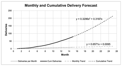
Figure 2.11 Example of Cumulative Forecasting Using a Quadratic Trend

Table 2.5 Example of Cumulative Forecasting Using a Quadratic Trend
For the Formula-philes: General solution of a quadratic equation
The general solution of any quadratic equation of the form ax2 + bx + c = 0 is:
Yes, that’s right, it’s another one of those things we did in school during mathematics classes but we couldn’t see its relevance to life as we knew it. Well, that’s another outstanding objective to cross off your list!
The procedure is simply:
- Identify the slope and intercept of the Best Fit straight line through the data, or the Best Fit polynomial (order 2) through the origin for the Cumulative data
Create the Quadratic equation for the Cumulative Value using the standard result derived in the previous two sections
Cumulative = n where m is the slope and c the intercept
- Apply the general solution of a quadratic equation to derive the desired solution for the sequence number (Build Number or Time Period) required
We may recall from school that a quadratic equation will have either 0, 1 or 2 solutions (or roots as they were called in class):
- 0. The sign under the square root is negative and so we cannot solve the equation (We are not going to delve into the murky waters of imaginary numbers, you'll be pleased to hear.)
- 1. An equation of the form (x - k)2 = 0 is a quadratic with two identical roots of x = k, so to all intents and purposes it only has one solution
- 2. This is probably the most common situation we will come across as estimators. However, we should be on our guard to select the right one — see the Formula-phobe discussion.
For the Formula-philes: Finding when a future Cumulative Value occurs

For the Formula-phobes: Quadratic equations generally have two solutions
Quadratic equations are symmetrical about some value and so have two solutions for the same value; we require the lowest positive value root as illustrated.
In the example here for the cumulative of an increasing straight line, there are two values at which Cum y = 100:
x = -25 and x = 16
However, in the case of a decreasing straight line, there may be two positive roots, in which case we will want the first, i.e. the lower of the two. In this case, when Cum y = 100:
x = 16 and x = 25
The reason that the Cumulative y value turns back on itself is that the underlying straight line has crossed the x-axis and the y values are all negative.


In this case we should question whether the underlying data line is truly linear, or whether it just appears linear for the data we have (a shallow curve might be being disguised by the data scatter).
Caveat augur
It is important that we recognise that any apparent straight-line relationship may only be valid in the context of the data in which we observe it. If the true relationship is in fact a shallow curve through our data, then a straight line might only be a good approximation to that curve in the range local to the data, which may not be the case if we extrapolate too far in either direction.
A word (or two) from the wise?
"The straight line: a respectable optical illusion which ruins many a man."
Victor Hugo Les Misérables (1862) French Novelist
Figure 2.12 illustrates the sentiments expressed by Victor Hugo (albeit in a different context, and not in French.) Here, the trend is slightly bowed around a straight line. Without the straight line as a reference, it is difficult to see.

Figure 2.12 Straight Line or Shallow Curve?
A corollary (or natural extension) to this exploits the difference property of two straight lines, which as we showed in Section 2.1.2, is also a straight line. Consequently, the cumulative difference between two straight lines is a quadratic function. This may be really useful to us if we have to estimate a recovery position to some plan. (And who hasn’t?)
Consider another example where we are behind schedule at the start of a programme, (does that sound all too familiar?) but that we aim to recover and are showing positive signs of doing so. Take the scenario in which the requirement or plan is to increase output linearly, but the reality is that we started later than planned, but are managing to increase output at a higher rate than originally planned. The procedure here is simply:
- Identify the slope and intercept of the planned linear output growth
- Identify the slope and intercept of the Best Fit straight line through the actual data
- Subtract the difference between the two slopes and the two intercepts (step ii minus step i) to get the Best Fit straight line through the difference. (Clearly, if the slope from step ii is less than step i, then stop here because we aren’t recovering – although we can still predict where we might end up!)
Generate the parameters of the Cumulative Quadratic Equation for the Cumulative difference to plan
Cumulative = where m is the slope and c the intercept
- Apply the general solution of a quadratic equation to derive the expected recovery position, i.e. when the Cumulative Difference is zero
Table 2.6 illustrates our situation against plan. Both the plan and our actual achievement here are linear, as shown in Figure 2.13 so this allows us to use the ‘straight line difference’ property to forecast the recovery position.
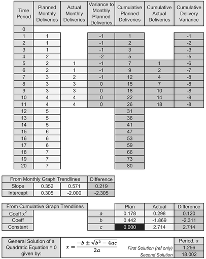
Table 2.6 Linear Trend Recovery Point Using a Cumulative Quadratic Trend
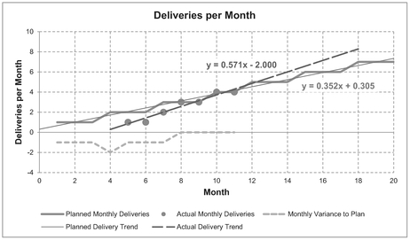
Figure 2.13 Finding the Cumulative Recovery Point to a Linear Plan (1)
From Figure 2.13 we can extract the slope and intercept for both ‘Best Fit’ trendlines, and calculate the difference between the two slopes and the two intercepts to get an equivalent straight line for the variance recovery. Note that we should resist the temptation to fit a straight line through the variance data as this is a composite curve covering the variance build-up and its recovery. (It gets worse before it gets better! In other words, it is only a straight line from the point at which recovery commences, in this case Month 4 or arguably Month 5.)
Figure 2.14 shows the Cumulative position of the linear data, to which we can fit Quadratic Trendlines. Note that we should impose an intercept of zero on the plan because we are assuming that the project starts at Month 0. However, in the case of the recovery we should leave the intercept unconstrained as we are not beginning recovery at Month 0 (i.e. Month 4 is the new Month 0).
We can now extract the coefficients for the x2 and x terms for both these curves, and the constant in the case of the recovery curve. In Table 2.6 we took the difference between the corresponding coefficients in order to get the equivalent Cumulative Variance Recovery Curve. Finally, we can use our rekindled favourite formula from school for the general solution of a quadratic equation to find when the recovery reaches zero. In this case we recover at Month 18.
We can adapt this technique to situations where the plan and the recovery profiles are not linear but the difference is linear.
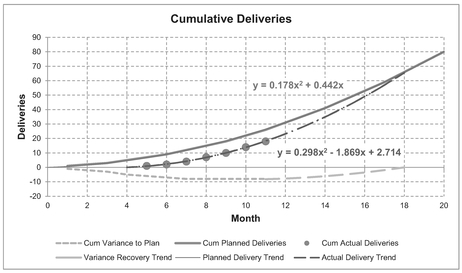
Figure 2.14 Finding the Cumulative Recovery Point to a Linear Plan (2)
OK, from your facial expression I can see that you want a period of personal recovery. Put the kettle on.
Example: Using the Quadratic Curve to Estimate a Missing Cumulative Value
Consider the situation in which data has been ‘lost’ during a migration from a legacy system to a new Enterprise Planning system (possibly because no-one remembered to ask the estimator what data was important to retain. Is my cynicism beginning to show again?) Suppose we know how many widgets we have made every month on a project since the new system was introduced, but not how many were made beforehand. (As usual we want the data now and cannot wait for the archive to be retrieved!) Suppose also that we know that we appear to be increasing output per week linearly from the data we do have and that the Project commenced ten weeks before the new system was implemented. (They weren’t going to wait just because the IT slipped, were they?)
If we plot the Cumulative number of Widgets Produced against ‘Months from Project Start’, we can fit a Quadratic Trendline in Excel but this time we should not constrain the intercept to be zero (that is only valid from the start of the series.) By projecting the Quadratic Trendline back to Month 0 we can get an estimate of the cumulative number of widgets ‘lost’ in the systems handover using the negative intercept.

From the example, the intercept of -1528 is an estimate of the number of widgets produced previously, and ‘lost’ in the systems migration.
2.3 Chapter review
In this chapter, we explored the humble straight line, which can be categorised as being either discrete or continuous linear functions in respect of the input variable (horizontal x-axis), and could be expressed as a function of any two points on the line. These two points allow us to define the slope or gradient of the line and where it intersects the vertical axis (intercept).
Where the straight line represents an estimating relationship in which the data values are independent of each other, then the only property of real note is that the implied best fit relationship is either increasing or decreasing monotonically (incessantly in one direction).
However, where the data points are not independent of each other, but form a natural data sequence, we may want to consider the cumulative value of those relationships. In these cases we found that the Cumulative Value sequence was always a Quadratic Function, whose coefficients were functions of the linear data’s slope and intercept. If the Cumulative Value sequence commenced with the first value in the linear sequence, then the Cumulative Value’s Quadratic Function passes through the origin. The inherent variability or scatter in the underlying linear trend will be naturally smoothed in the cumulative perspective. Robert Henri (attributed by Cipra, 1998) may have
A word (or two) from the wise?
"A curve does not exist in its full power until contrasted with a straight line."
Robert Henri (1865-1929) American Realist Painter and Educator
been referring to curves and lines in an artistic sense rather than the mathematical sense employed here, but the same observation can be made. After all is Estimating not part art as well as science?
We discovered that the Cumulative Quadratic property allows us to consider data where we have sequential data, but not necessarily fixed sequential interval reporting periods – which could mask that there is an underlying linear relationship. We may typically report data in fixed time periods which do not necessarily reflect that the profiling of the data (ramp up/ramp down) in question.
We explored the power of this property (no pun intended, honestly) and how we might use cumulative data as a smoothing function where we have erratic data, or how in some circumstances we can use it to estimate missing data. We concluded with a foray into our past lives and discovered that there really was a use for the general solution of a quadratic equation that we studied in school . . . and wondered why we had. Well, we know now it was in the syllabus to help prepare us all to be estimators or forecasters!
Reference
Cipra, BA (1998) ‘Strength Through Connections at IMA’, Philadelphia, SIAM News, Vol 31 No 6, July/August.