
3. Realizing Machine Learning Algorithms with Spark
This chapter discusses the basics of machine learning (ML) first and introduces a few algorithms, such as random forest (RF), logistic regression (LR), and Support Vector Machines (SVMs). It then goes on to elaborate how ML algorithms can be built over Spark, with code sketches wherever appropriate.
Basics of Machine Learning
Machine learning (ML) is the term that refers to learning patterns in the data. In other words, ML can infer the pattern or nontrivial relationship between a set of observations and a desired response. ML has become quite common—for example, Amazon uses ML to recommend appropriate books (or other products) for users. These are a type of ML known as recommender systems. Recommender systems learn the behavior of users over time and predict the product(s) a user might be interested in. Netflix also has recommender systems for videos, as do most online retailers, such as Flipkart. The other applications of ML include these:
• Speech/voice identification system: Given a database of past tagged speeches (with users) and a new speech, can we recognize the user?
• Face recognition systems for security: Given a database of tagged images (with people) and a new image, can we recognize the person? This can be seen to be a classification problem. A related problem is known as verification—given a database of tagged images (with people) and a new image with claimed person identification, can the system verify the identity? Note that in this case, it is a yes/no answer.
• A related yes/no answer is useful for spam filtering: Given a set of emails tagged as spam and not-spam and a new email, can the system identify whether it is spam?
• Named entity recognition: Given a set of tagged documents (with entities tagged) and a new document, can the system name the entities in the new document correctly?
• Web search: How can we find documents that are relevant to a given query from the billions of documents available to us? Various algorithms exist, including the Google page rank algorithm (Brin and Page 1998) and others, such as RankNet, an algorithm that the authors claimed could outperform Google’s PageRank algorithm (Richardson et al. 2006). These depend on domain information as well as the frequency with which users visit web pages.
Machine Learning: Random Forest with an Example
Most textbooks on ML use this example to explain the decision trees and subsequently the RF algorithm. We will also use the same, from this source: www.cs.cmu.edu/afs/cs.cmu.edu/project/theo-20/www/mlbook/ch3.pdf.
Consider the weather attributes outlook, humidity, wind, and temperature with possible values:
• Outlook: Sunny, overcast, and rain
• Humidity: High, normal
• Temperature: Hot, mild, and cool
The target variable is PlayTennis with possible values Y and N. The idea is that based on past data, the system learns the patterns and is able to predict the outcome given a particular combination of the attribute values. The historical data is given in Table 3.1.
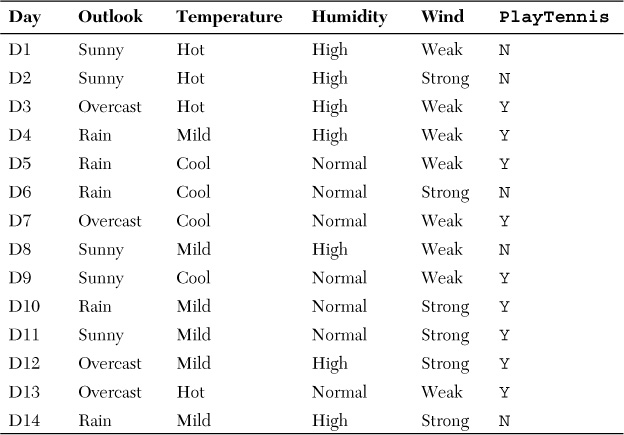
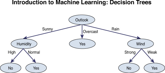
A simple solution to learn this pattern is to construct a decision-tree representation of the data. The decision tree can be understood as follows: Nodes of the decision tree are attributes, and branches are possible attribute values. The leaf nodes comprise a classification. In this case, the classification is Y or N for the PlayTennis prediction variable. The decision tree looks as shown in Figure 3.1.
There are theoretical aspects of decision trees—top induction processes to construct the tree as well as measures such as entropy and gain that help in deciding which attribute must be at the root. But we will not go into those details. The idea is to get a feel for ML with the intuitive example. Decision trees as well as RFs are inherently parallelizable and are well suited for Hadoop itself. We will go deeper into the other algorithms such as LR, which are of interest for us due to their iterative nature. These necessitate beyond-Hadoop thinking.
It must be kept in mind that decision trees have certain advantages such as their robustness to outliers, the handling of mixed data, and their parallelization scope. The disadvantages include the low prediction accuracy, high variance, and size versus goodness of fit trade-off. Decision trees might require pruning in order to avoid overfitting the data (which can result in poor generalization performance). A generalized form is known as the random forest, which is a forest of trees. A forest can be built as a set of multiple decision trees and avoid pruning for generalization. The final outcome of the RF algorithm is the mean value in case of regression or the class with maximum votes for classification. The RF algorithm also has greater accuracy across domains compared to the decision tree. The book Introduction to Machine Learning (Smola and Vishwanathan 2008) has an excellent treatment of the basics of ML. This book is available at http://alex.smola.org/drafts/thebook.pdf.
The taxonomy of ML algorithms based on the kind of learning problems is as follows:
• Inductive versus transductive: The inductive approach is to build a model from the training examples and use the model to predict the outcomes for the test data. This is how the majority of ML approaches work. However, in cases in which the training data is meager, there is a possibility of the inductive approach resulting in a model with poor generalization. A transductive approach might be better in such cases. Transduction does not actually build any model, but only creates a mapping from a set of training examples to a set of test examples. In other words, it attempts to solve only a weaker problem and not a more general one.
• Learning approach: Based on the learning approaches, ML may be classified as one of the following:
• Supervised learning: There is a set of labeled data for training—which implies, for example, in the case of classification problems, training data comprises data and the classes to which they belong (labels). Binary classification is the fundamental problem solved by ML—that is, which of two categories does the test data belong to? This can be used to classify email as spam or nonspam, given a set of emails labeled as spam and nonspam and the new email required to be classified. Another application might be to predict whether an owner will default on a loan in the case of home loans, given his credit and employment history as well as other factors. Multiclass classification is a logical extension of the binary classification, where the output space can be a set range of different values. For example, in the case of Internet traffic classification, the page under question could be classified as sports, news, technology, or adult/porn, and so on. The multiclass classification is a harder problem that can sometimes be solved by an ensemble of binary classifiers, or it might require multivariate decision models.
• Reinforcement learning: The machine interacts with its environment by producing a series of actions. It gets a series of rewards (or punishments). The goal of the ML is to maximize the rewards it gets in the future (or minimize future punishments).
• Unsupervised learning: There are neither labeled data for training nor any rewards from the environment. What would the machine learn in this case? The goal is to make the machine learn the patterns of data and be useful for future predictions. Classic examples of unsupervised learning are clustering and dimensionality reduction. Common clustering algorithms include k-means (based on centroid models), a mixture of Gaussians, hierarchical clustering (based on connectivity models), and an expectation maximization algorithm (which uses a multivariate normal distribution model). The various dimensionality reduction techniques include the factor analysis, principal component analysis (PCA), independent component analysis (ICA), and so forth. The Hidden Markov Models (HMMs) have been a useful approach for unsupervised learning for time-series data (Ghahramani 2004).
• Data presentation to learner: Batch or online. All data is given at the start of learning in the batch case. For online learning, the learner receives one example at a time, outputs its estimate, and receives a correct value before getting the next example.
• Task of ML: Regression or classification. As stated before, classification could be multiclass or binary. Regression is a generalization of classification and is used to predict real-valued targets.
Logistic Regression: An Overview
Logistic regression (LR) is a type of probabilistic classification model used to predict the outcome of a dependent variable based on a set of predictor variables (features or explanatory variables). A common form of LR is the binary form, in which the dependent variable can belong to only two categories. The general problem where the dependent variable is multinomial (not binary) is known as multinomial LR, a discrete choice model, or a qualitative choice model. LR measures the relationship between the categorical dependent variable and one or more dependent variables, which are possibly continuous. LR computes the probability scores of the dependent variable. This implies that the LR is more than just a classifier—it can be used to predict class probabilities.
Binary Form of LR
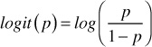
LR is used to predict the odds ratio based on the features; the odds ratio is defined as the probability that a specific outcome is a case divided by the probability that it is a noncase. LR can make use of continuous or discrete features, similar to linear regression. But the main difference is that LR is used to make a binary prediction, unlike linear regression, which is used for continuous outcomes. To create a continuous criterion as a transformation of the features, the LR takes the natural logarithm of the dependent variable being a case (referred to as logit or log-odds). In other words, LR is a generalized linear model, meaning it uses a link function (logit transformation) on which linear regression is performed. Given this, LR is a generalized linear model, meaning it uses a link function to transform a range of probabilities into a range from negative infinity to positive infinity.
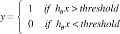
Despite the probabilistic framework of LR, all that LR assumes is that there is one smooth linear decision boundary. It finds that linear decision boundary by making assumptions on the P(Y|X) to take some form, such as the inverse logit function applied to a weighted sum of the features. Then it finds the weights by a maximum likelihood estimation (MLE) approach. So if we try to solve the classification problem ignoring the fact that y is discrete-valued, and use the linear regression algorithm to try to predict y given x, we’ll find that it doesn’t make sense for the hypothesis hθ(x) to take values larger than 1 or smaller than 0 when we know that y ∊ {0, 1}, where y is the dependent variable and x the features. To fix this, the new hypothesis hθ(x) is chosen which is nothing but a logistic1 or sigmoid function:
1 Logistic function: Inversed Logit function
therefore, logistic function
Therefore, the new hypothesis becomes this:
Now, we predict:
If we plot the preceding function, we can see g(z) →1 as z → ∞ and similarly g(z) → -1 as z → -∞. Therefore, g(z) and hθ(x) are bound between 0 and 1.
Let us assume that
p(y | x; θ) = (hθ(x))y (1 – hθ(x))1 – y
So the likelihood of the parameters can be written as
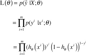
Since maximizing the log of the likelihood will be easier:
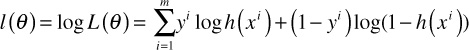
Now, this log likelihood function can be maximized using gradient descent, stochastic gradient descent (SGD), or some other optimization techniques.
A regularization term can be introduced to avoid overfitting. There are two types of regularization, L1(Laplace prior) and L2(Gaussian prior), which can be used based on the data and application.
Logistic Regression Estimators
LR predicts probabilities, rather than just classes. This implies that LR can be fitted with a likelihood function. However, no closed-form solution exists for the coefficient values that maximize such a function. So estimators come into the picture. We can solve the function approximately using an iterative method, say, the Newton’s method (more precisely, Newton-Raphson) (Atkinson 1989). It has been shown that Newton’s method, also named as iteratively reweighted least squares, performs better than others for solving LR (Minka 2003). The process starts with an approximate solution, revises it slightly, and checks whether the solution improved. This process ends when improvements over successive iterations are too small. The model might not converge in some instances, if there was a large number of predictors compared to cases, if there was sparse data, or if there is a high correlation between predictors.
Multinomial Logistic Regression
A generalization of the binary LR to allow more than two discrete outcomes is known as multinomial LR or multinomial logit. A classifier realized using a multinomial logit is often referred to as the maximum entropy classifier or MaxEnt for short. MaxEnt is an alternative to a Naive Bayes classifier, which assumes that the predictors (features) are independent. The MaxEnt does not make this rather strong assumption, making it applicable to a wider set of scenarios when compared to the Naive Bayes classifier. However, learning in a Naive Bayes classifier is much easier and involves only counting up the number of feature-class co-occurrences. In MaxEnt, learning the weights is more involved—it might require an iterative procedure for the same. This is because the weights are maximized using a Maximum A-Posteriori (MAP) estimation. It must be noted that the multinomial logistic model can be viewed as a sequence of conditional binary logistic models.
Logistic Regression Algorithm in Spark
JavaHdfsLR is a Spark-based implementation of an LR–based classification algorithm using models trained by SGD. As indicated previously, the likelihood function can be estimated using SGD in addition to approximation methods such as Newton-Raphson. The input data set and output results are both files in the Hadoop Distributed File System (HDFS), which exhibits the seamless HDFS support that Spark offers. The flow of computation can be traced as follows, starting from the main file:
1. Create a Resilient Distributed Dataset (RDD) from the input file in HDFS. The code sketch is as follows:
......
String masterHostname = args[0];String sparkHome = args[1];
String sparkJar = args[2]; String outputFile = args[3];
String hadoop_home = args[4];
// initialize a JavaSparkContext object
JavaSparkContext sc = new JavaSparkContext(args[0], "JavaHdfsLR",
sparkHome , sparkJar);
// create the input file url of HDFS
String inputFile = "hdfs://" + masterHostname + ":9000/" + args[1];
// create an RDD from the input file stored in HDFS
JavaRDD<String> lines = sc.textFile(inputFile);
........
2. Apply transformation “ParsePoint” using the map() function, which is a Spark construct, similar to what we have as map in the Map-Reduce framework. This parses each input record into individual feature values required for the calculation of weights and gradient.
ParsePoint function invocation in main:
JavaRDD<DataPoint> points = lines.map(new ParsePoint()).
cache();
Actual ParsePoint transformation:
static class ParsePoint extends Function<String, DataPoint>
{
public DataPoint call(String line) {
// tokenize the input line on space character
StringTokenizer tok = new StringTokenizer(line, " ");
// first entry is assigned to the variable "y" of the DataPoint object
double y = Double.parseDouble(tok.nextToken());
// a list of the remaining ones forms the variable "x" of the DataPoint object
double[] x = new double[D];
int i = 0;
// create the list by iterating the "number of Dimensions" times
while (i < D) {
x[i] = Double.parseDouble(tok.nextToken());
i += 1;
}
return new DataPoint(x, y);
}
}
3. Iterate as many times as there are features present in the input records, to create a list of initial weights.
4. Calculate the gradient using another map transformation (equivalent to the mathematical formula shown previously), by iterating the user-specified number of times. With every iteration, the calculated gradient is summed up in its vector form using the reduce transformation, to achieve the final value for the gradient. This is used to adjust the initial weight to obtain the calculated weight for the input record, which is the final result.
Computer gradient class:
static class ComputeGradient extends Function<DataPoint, double[]> {
double[] weights;
public ComputeGradient(double[] weights) {
this.weights = weights;
}
public double[] call(DataPoint p) {
double[] gradient = new double[D];
// iterate 'D' times to calculate the gradient for all the dimensions of the data point
for (int i = 0; i < D; i++) {
double dot = dot(weights, p.x);
gradient[i] = (1 / (1 + Math.exp (-p.y * dot)) - 1) * p.y * p.x[i];
}
return gradient;
}
}
/*
* Utility method used within ComputeGradient for
* calculating the product of the dimension of two
* vectors
*/
public static double dot(double[] a, double[] b) {
double x = 0;
for (int i = 0; i < D; i++) {
x += a[i] * b[i];
}
return x;
}
Iterating through the gradient:
for (int i = 1; i <= ITERATIONS; i++) {
// calculate the gradient per iteration
double[] gradient = points.map(
new ComputeGradient(w)
).reduce(new VectorSum());
// adjust the initial weight accordingly
for (int j = 0; j < D; j++) {
w[j] -= gradient[j];
}
Support Vector Machine (SVM)
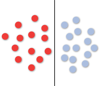
The SVM is a supervised learning method for the binary classification problem. Given a set of objects/points that fall into two categories (training data), the question arises as to how to classify the given new point (test data) into one of the two categories. The SVM learning method computes the line/plane that separates the two categories. For example, in a simple case, in which the points are linearly separable, the SVM line looks as shown in Figure 3.2.
Complex Decision Planes
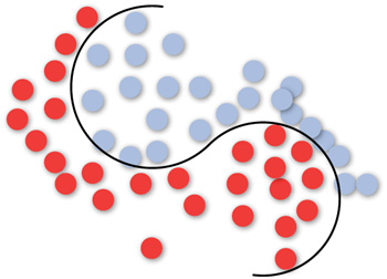
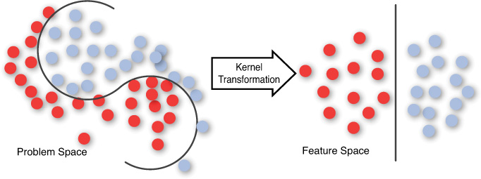
Many classification problems are not linearly separable and might require complex decision planes for optimal separation of the categories. The nonlinear (curve) separation case is illustrated in Figure 3.3. In this case, it is clear that the points/objects are not linearly separable and need a curve to separate them. The SVMs are typically good for classification problems that are plane-separable, known as hyperplane classifiers. However, the beauty of SVM is that even if the classes are not linearly separable in the problem space, it can still treat it as a hyperplane problem in the feature space.
The power of SVM can be understood from the illustration in Figure 3.4. It can be observed that using a series of mathematical functions known as kernels, the problem space is transformed into what is known as the feature space, multidimensional space, or infinite space. The problem becomes linearly separable in the feature space. It must be noted that SVM finds the optimal hyperplane, meaning that the distance to the nearest training data point (functional distance, not Euclidean) for both classes is maximal to make the generalization error of the classifier lower. The key insight used in SVMs is that the higher dimension space does not have to be dealt with directly, but only the dot product in that space is required. SVMs have also been extended to solve regression tasks in addition to binary classification.
Mathematics Behind SVM
The mathematics used in this section is derived from Boswell’s 2002 paper. We are given l training samples {xi, yi}, where xi refers to the input data with dimension d, and yi is a class label signifying which class the input data belongs to. All hyperplanes in the input space are characterized by the vector w and a constant b expressed as
w · x + b = 0
Given such a hyperplane (w, b) that separates the data, this gives the function that defines the hyperplane and can classify the data as required:
f(x) = sign(w · x + b)
We then define the canonical hyperplane as
yi(xi · w + b) ≥ 1 ∀ i
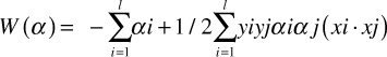
Given a hyperplane (b, w), we can see that all pairs {γb, γw} define the same hyperplane, but each with a different functional distance to a given data point. Intuitively, we are looking for the hyperplane that maximizes the distance from the closest data points. Effectively, we need to minimize W(α) where
subject to the conditions
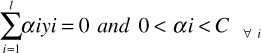
where C is a constant and α is a vector of l nonnegative Lagrange multipliers to be determined. It can be seen that, finally, the optimal hyperplane can be written as
It can also be shown that
αi (yi (w · xi + b) – 1) = 0 ∀ i
In other words, when the distance of an example is greater than 1, α = 0. So only the closest data points contribute to w. Those training examples for which αi > 0 are termed as support vectors. This is the reason this learning process came to be known as SVMs because it is anchored on the support vectors. αi can be thought of as the measure of how well it represents the example—how important was this example in determining the hyperplane. The significance of the constant C is that it is a tunable parameter. A higher value of C implies more learning from the training vector and consequent overfitting, and a lower value of C implies more generality.
We now explore the use of the kernels in SVM. As stated before, the purpose of using the kernel functions is to transform the input space with nonlinearly separable data into a feature space, where the data is linearly separable. We define a mapping z = θ(x) that transforms the input vector into a higher dimensional vector z. It turns out that all occurrences of x could be replaced with θ(x) in equation 1 and we end up with an equation for w that is
and f(x) can be written as
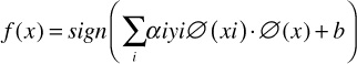
This implies that if we do not need to deal with the mapping z = θ(x) directly, we only need to know the dot product K(xa,xb) = θ(xi) θ(xj) in the feature space. Some useful kernels that have been discovered include the polynomial kernel, Gaussian Radial Basis Function (RBF), and hyperbolic tangent, among others.
It might be possible to solve a multiclass classification problem by using an ensemble of SVMs and comparing the classification of each class with all others (Crammer and Singer 2001).
SVM in Spark
The implementation makes use of another inner class called SVMModel representing the model object returned from the training process along with SVMWithSGD, which is the core implementation behind SVM. The code can be found in the ML-Lib trunk of the Spark source itself. A brief description is given in the text that follows.
Following is the workflow of SVM algorithm:
1. Create the Spark context.
2. Load Labeled input train data; labels used in SVM should be {0, 1}.
3. Train the model using the input RDD of (label, features) pairs and other input parameters.
4. Create an object of type SVMWithSGD using the inputs.
5. Invoke the overridden implementation of GeneralizedLinearModel’s run() method, which runs the algorithm with the configured parameters on an input RDD of LabeledPoint entries and processes the initial weights for all the input features.
6. Obtain an SVM model object.
7. Stop the Spark context.
PMML Support in Spark
Predictive Modeling Markup Language (PMML) is the standard for analytical models defined and maintained by the Data Mining Group (DMG), an independent consortium of organizations.2 PMML is an XML-based standard that allows applications to describe and exchange data mining and ML models. The PMML version 4.x allows both data munging (data munging is a term that refers to manipulations/transformations on data to make it usable by ML) and analytics to be represented in the same standard. PMML 4.0 added significant support for representing data munging or preprocessing tasks. Both descriptive analytics (that typically explains past behavior) and predictive analytics (that is used to predict future behavior) can be represented in PMML. We will restrict ourselves to the PMML 4.1, which is the recent standard as of November 2013, in the following explanation.
2 Some of the contributing members of this organization include IBM, SAS, SPSS, Open Data Group, Zementis, Microstrategy, and Salford Systems.
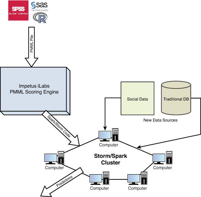
Figure 3.5 gives an overview of the PMML support we have developed for Spark/Storm. It illustrates the power of the paradigm of supporting PMML in both Spark and Storm. A data scientist typically develops the model in his traditional tools (SAS/R/SPSS). This model can be saved as a PMML file and consumed by the framework we have built. The framework can enable the saved PMML file to be scored (used for prediction) in batch mode over Spark—this gives it the power to scale to large data sets across a cluster of nodes. The framework can also score the PMML in real-time mode over Storm or Spark streaming. This enables their analytical models to work in real time.
PMML Structure
The PMML structure is captured in Figure 3.6 (Guazzelli et. al 2009b).
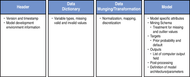
PMML Header
The first part is the header information, which captures version and timestamp details. It also carries details of the model development environment. An example is shown here in the XML form:
<Header copyright = "Impetus, Inc."
Description = "This is a Naive Bayes model expressed in
PMML">
<Application name = "Impetus Real Time Analytics
Environment" Version = "3.7"/>
<Timestamp>2013-11-29</Timestamp>
</Header>
Data Dictionary
The data dictionary contains the definition for each data field used by the model. The fields can be specified as continuous, categorical, or ordinal. Based on the type, appropriate ranges and data types (string or double) can be specified.
In the example given shortly, the categorical field class can take values Republican or Democrat. If this field were to be carrying a different value, it would be treated as an invalid value. NULL values are considered to be equivalent to missing values.
The variable V3 is of type continuous—it is a double with possible range {-1.0..+1.0}. It can be specified as shown in the following code:
<DataDictionary numberOfFields="4">
<DataField name="Class" optype="categorical"
dataType="string">
<Value value="democrat"/>
<Value value="republican"/>
</DataField>
<DataField name="age-group" optype="categorical"
dataType="string">
<Value value="old"/>
<Value value="youth"/>
<Value value="middle-age"/>
</DataField>
<DataField name="location" optype="categorical"
dataType="string">
<Value value="east"/>
<Value value="west"/>
<Value value="central"/>
</DataField>
<DataField name="V3" optype="continuous"
dataType="double">
<interval closure ="closedOpen"
leftMargin = "-1.0" rightMargin="1.0"/>
</DataField>
</DataDictionary>
Data Transformations
The different data transformations that can be specified in a PMML are the following:
• Continuous Transformation: This allows a continuous variable to be transformed into another continuous variable, mimicking normalization. An example is given here:
<LocalTransformations>
<DerivedField name="DerivedV3"
Datatype="double" optype="continuous">
<NormContinuous field = "InputV1" mapMissingTo="0"
outliers="asMissingValues">
<LinearNorm orig="1.7" norm="0">
<LinearNorm orig="11.7" norm="1">
</NormContinuous>
</DerivedFiled>
</LocalTransformations>
• Discrete Normalization: This allows string values to be mapped to numeric values. This is usually done for mathematical functions in regression or neural network models. An example follows:
IF ageGroup == "Youth"
THEN
DerivedAge = 1
ELSE
IF ageGroup = "Middle-Age"
THEN
DerivedAge=2
ELSE
DerivedAge=3
• Discretization: This is used to map continuous values to discrete string values, usually based on the range of values it can possibly take:
<LocalTransformations>
<DerivedField name="DerivedV4"
Datatype="string" optype="categorical">
<Discretize field = "InputV1" defaultValue="inter">
<DiscretizeBin binValue ="negative">
<Interval closure = "openClosed"
rightMargin = "-1" />
</DiscretizeBin>
<DiscreteBin binValue="inter">
< Interval closure = "openClosed"
leftMargin= "-1"
rightMargin="1"
</DiscretizeBin>
<DiscreteBin binValue="positive">
< Interval closure = "openOpen"
leftMargin= "1"
rightMargin="10"
</DiscretizeBin>
</DiscretizeField>
</DerivedFiled>
</LocalTransformations>
• Value Mapping: This is used to map discrete string values to other discrete string values. This is usually done by having a table (this could be outside of the PMML code and can be referenced from the code) specify the input combinations and the corresponding output for the derived variable.
Model
This element contains the definition of the data mining or predictive model. It also allows describing model-specific elements. The typical model definition for the regression model is:
<RegressionModel
modelName="VajraBDARegressionModel"
functionName="regression"
algorithmName="logisticRegression"
normalizationMethod="loglog"
</RegressionModel>
Mining Schema
This element is used to list all fields used in a model and can be a subset of the fields defined in the data dictionary element. It typically contains the following fields as a list of attributes:
• Name: Must refer to a field in the data dictionary element.
• usageType: Can be active, predicted, or supplementary; differentiates fields as being features or predicted variables.
• Outliers: Can be asMissingValues or asExtremeValues or asIs (default) value; indicates the treatment to be given to the outliers.
• lowValue and highValue: Used along with the outlier attribute.
• missingValueReplacement: Used for special treatment of missing values, by replacement with prespecified values.
• missingValueTreatment: Can be value, mean, or median, indicating how missing values are to be treated.
• invalidValueTreatment: Can be asIs, asMissing, or returnInvalid, indicating how invalid feature values are handled.
Targets and Outputs
The element Target is used to manipulate the value predicted by a model. It is usually used for post-processing—things like specifying default values of probabilities, which can be useful in case the model is unable to predict the probability, say, due to missing values. The priorProbability attribute of the Target element is useful for this purpose.
The output element is used for post-processing of predicted variables. With PMML 4.1, the entire set of preprocessing custom and built-in functions are also available for post-processing using the Output element. These include being able to specify default predicted values, distance or similarity measures of the record to the predicted entity (through the affinity attribute), ranking (useful in association models or k-nearest neighbor models), and so forth. For more details on PMML, please refer to the book by Alex Guazzelli (2009a).
PMML Producers and Consumers
A PMML producer is any entity that can create a PMML file. The traditional statistical modeling tools such as SAS/SPSS/R are PMML producers—they allow the user to save the analytical model as a PMML file. PMML consumers are those entities that can consume a PMML file and produce a prediction output or scoring output. Both R and SAS, as well as recent ones such as BigML, are PMML producers only, implying that they do not have support for consuming or scoring a PMML model. SPSS, Microstrategy, and recent ones such as KNIME have support for both producing and consuming PMML files.
Among the popular open source PMML consumers, Augustus was prominent and among the first to provide realizations for PMML specifications. Augustus can act as both PMML producer and PMML consumer. In the PMML consumer role, Augustus works beyond the limitations of memory, which is a constraint in traditional PMML scoring systems.
Concurrent Systems Inc., a big data startup, built a PMML scoring engine known as “Pattern” that works over a Hadoop cluster. This enables the PMML models to be scored over large data sets beyond the memory limitations of the cluster by consuming data sources from the HDFS (Bridgwater 2013). Some limitations do exist with both Augustus and Pattern in that they do not support a large variety of PMML models.
JPMML is another open source PMML producing and consuming engine, completely written in Java. The JPMML has support for a wide variety of PMML models, including the RandomForests, the Association, clustering, Naive Bayes, general regression, k-nearest neighbors, SVMs, and so on. The JPMML is available free from https://github.com/jpmml/jpmml.
The ADAPA work from Zementis Inc., another big data startup, is also popular and is available via the Amazon Web Services (AWS) at the AWS marketplace. ADAPA was one of the earliest PMML scoring engines that worked over Hadoop (Guazzelli et al. 2009a). It has evolved into the Universal PMML Plug-in (UPPI) recently. ADAPA can be viewed as a real-time PMML scoring platform, and UPPI is the batch equivalent over Hadoop.
PMML Support in Spark for Naive Bayes
We will quickly explain the Naive Bayes algorithm, before explaining how it works in Spark. The simple equation for the Bayes theorem is
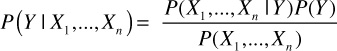
where X1,X2...,Xn are the features, and Y is a class variable with a small number of possible outcomes or classes.
In other words, to put it in simple English,
Since the denominator is likely to be a constant in practice, the numerator of the earlier equation is important to classify the data. The Naive Bayes algorithm makes the “conditional independence” assumption, which states that each feature is conditionally independent of every other feature given the category Y:
where Z (the evidence) is a scaling factor. The class prior and feature probability distributions can be approximated to the relative frequencies from the training set, which would be maximum likelihood estimates of the probabilities.
The essence of realizing support for Naive Bayes PMML is to have the Naive Bayes algorithm itself implemented in Spark. The implementation must also read the PMML for the model parameters and perform any preprocessing necessary. The code for the same, a Naive Bayes PMML scoring in Spark, is shown in Appendix A, “Code Sketches.” It skips the preprocessing steps to focus on the scoring over Spark. The steps for executing the previous as a Spark application are given here:
1. Create an object of the SAX Parser and a Naive Bayes handler object that would be used for predicting the category using the PMML model file.
2. Generate a Java RDD from the input file. Preprocess the input RDD elements to get an RDD containing elements, each of which is an array of input record dimensions for a record.
3. Iterate through the elements of the processed RDD, to predict the category to which they belong using the Naive Bayes handler object created in step 1. Also, simultaneously log the predicted category to an output file.
4. Finally, the time taken to accomplish the classification process is logged in the output file.
PMML Support in Spark for Linear Regression
The linear regression is an algorithm that uses the supervised learning model to understand the relationship between a scalar variable (y) and a set of features or explanatory variables, denoted by X. Like other regression algorithms, linear regression focuses on probability distribution of y given X, rather than on the joint distribution of y and X (which would be a multivariate analysis). It has been studied quite extensively and used in a number of applications, primarily because linear dependence of y on the features is easier to model than nonlinear dependence. The common form of linear regression is expressed as
y = w0 + w1x1 + w2x2+...wnxn
where w0, ... wi are the weights (parameters) that are learned by the training examples. In other words, y = wTx. The mean squared error can be defined as
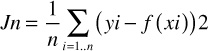
The goal is to find the weights that minimize the error function. In matrix form, we get the final equation as w = (XTX)-1XTy. Ultimately, linear regression is all about solving a set of linear equations—which implies that gradient descent methods or numerical methods can be used to solve the same.
The essence of realizing support for linear regression PMML is to have the linear regression algorithm itself implemented in Spark. The implementation must also read the PMML for the model parameters and perform any preprocessing as necessary. The code for the same, a Linear Regression PMML scoring in Spark, is shown in Appendix A. It skips the preprocessing steps to focus on the scoring over Spark. The steps for executing the previous as a Spark application are given here:
1. Load the PMML model from the given input pmml file. This is used to instantiate an object of RegressionModelEvaluator type, which further facilitates the classification process. This instantiation of the object itself completes the “training phase” of the algorithm.
2. For testing of the model, an RDD is created from the input file whose location is specified by the user.
3. Apply a map() transformation to the generated RDD, where the input line is split on “,” to obtain the individual dimensions of the record. After that, the dimension values are used to create a HashMap required by the evaluate() method of the RegressionModelEvaluator object to evaluate the species.
4. Outside of the transformation, the prediction list is obtained through a Spark action applied to the resultant RDD.
5. Finally, the results and the time taken to accomplish the classification process are logged in the output file.
Machine Learning on Spark with MLbase
The main motivation for MLbase is the need to make ML available to a wide set of people, who might not have a strong background in distributed systems and might not have the programming expertise to realize the ML algorithms at scale. MLbase uses a new Pig Latin–like declarative interface to specify the ML tasks along with the data loading part—for example:
var X = load("imp_insurance_data", 2 to 15)
var y = load("imp_insurance_data", 1)
var (fn-model, summary) = doClassify(X, y)
The preceding code shows how to load a file into the MLbase environment. It constructs the feature set as comprising the columns numbered 2 to 15 in the data set, while the first column (predictor variable) is set to the y variable in the next line. The third line performs an appropriate classification for this data and returns the model as a Scala function. It also returns a summary of the model and the lineage of the model (its learning process). It can be seen that it does not specify the precise classification algorithm to be used. MLbase typically chooses its own algorithms and parameters, as well as deciding where and how to execute them across the cluster.
MLbase can also be viewed as a set of primitives to build new distributed ML algorithms. The primitives currently available are gradient and SGD, divide and conquer primitives for matrix factorization (Kraska et al. 2013), and graph processing primitives similar to GraphLab (Low et al. 2010). To date, several algorithms such as k-means clustering, LogitBoost, and SVMs have been realized over these primitives. It also allows an ML expert to inspect the execution plan in detail and fix the algorithms and parameter ranges, ideal for experimentation.
The architecture of MLbase is a master-slave one. The user sends requests (in the form given previously) to the master. The master parses the request and generates a logical learning plan (LLP). The LLP is a workflow explaining the ML task in the form of a combination of ML algorithms and their parameters, as well as the featurization techniques and data subsampling strategies. The LLP is then converted into a physical learning plan (PLP), which comprises a series of ML operations designed over the primitives of MLbase. The master distributes the PLP into the set of slaves for execution. For a classification task, the LLP can comprise subsampling to first get a smaller data set, and then explore different combinations of the SVM or AdaBoost techniques along with the parameters such as regularization. After initial testing of the quality of results, the LLP gets converted into a PLP, which specifies the appropriate algorithm and parameters to be trained on a large sample.
References
Atkinson, Kendall E. 1989. An Introduction to Numerical Analysis. John Wiley & Sons, Inc. Hoboken, NJ, USA.
Boswell, Dustin. 2002. “Introduction to Support Vector Machines.” Available at http://dustwell.com/PastWork/IntroToSVM.pdf.
Bridgwater, Adrian. 2013. “Scoring Engine Via PMML Makes Hadoop Easier.” Dr. Dobbs Journal. Available at www.drdobbs.com/open-source/scoring-engine-via-pmml-makes-hadoop-eas/240155567.
Brin, Sergey, and Lawrence Page. 1998. “The Anatomy of a Large-Scale Hypertextual Web Search Engine.” In Proceedings of the Seventh International Conference on World Wide Web 7 (WWW7). Philip H. Enslow, Jr. and Allen Ellis, eds. Elsevier Science Publishers B. V., Amsterdam, The Netherlands, 107-117.
Crammer, Koby, and Yoram Singer. 2001. “On the Algorithmic Implementation of Multiclass Kernel-based Vector Machines.” Journal of Machine Learning Research 2:265-292.
Guazzelli, Alex, Kostantinos Stathatos, and Michael Zeller. 2009a. “Efficient Deployment of Predictive Analytics Through Open Standards and Cloud Computing.” SIGKDD Exploration Newsletter 11(1):32-38.
Guazzelli, Alex, M. Zeller, W. Chen, and G. Williams. 2009b. “PMML: An Open Standard for Sharing Models.” The R Journal 1(1).
Ghahramani, Zoubin A. 2004. “Unsupervised Learning,” Advanced Lectures on Machine Learning. Lecture Notes in Computer Science, Editors Bousquet, Olivier, Luxburg, Ulrike, and Rätsch, Gunnar. Springer-Verlag, Heidelberg, 72-112.
Kraska, Tim, Ameet Talwalkar, John Duchi, Rean Griffith, Michael J Franklin, and Michael Jordan. 2013. “MLbase: A Distributed Machine-Learning System.” In Conference on Innovative Data Systems Research, California. Available at http://www.cidrdb.org/cidr2013/program.html.
Low, Y., J. Gonzalez, A. Kyrola, D. Bickson, C. Guestrin, and J. M. Hellerstein. 2010. “Graphlab: A New Parallel Framework for Machine Learning.” In Proceedings of Uncertainty in Artificial Intelligence (UAI). AUAI Press, Corvallis, Oregon, 340-349.
Minka, T. 2003. “A Comparison of Numerical Optimizers for Logistic Regression.” Technical Report, Dept. of Statistics, Carnegie Mellon University, Pittsburg, USA.
Richardson, Matthew, Amit Prakash, and Eric Brill. 2006. “Beyond PageRank: Machine Learning for Static Ranking.” In Proceedings of the 15th International Conference on World Wide Web (WWW ‘06). ACM, New York, NY, 707-715.
Smola, Alexander J. and S.V.N. Vishwanathan. 2008. Introduction to Machine Learning. Cambridge University Press, Cambridge, UK. Available at http://alex.smola.org/drafts/thebook.pdf.