7

Phylogenetics

Phylogenetics is the application of molecular sequencing that is used to study the evolutionary relationship among organisms. The typical way to illustrate this process is through the use of phylogenetic trees. The computation of these trees from genomic data is an active field of research with many real-world applications.

In this book, we will take the practical approach that is mentioned to a new level: most of the recipes here are inspired by a recent study on the Ebola virus, researching the recent Ebola outbreak in Africa. This study is called Genomic surveillance elucidates Ebola virus origin and transmission during the 2014 outbreak, by Gire et al., published in Science. It is available at https://pubmed.ncbi.nlm.nih.gov/25214632/. Here, we will try to follow a similar methodology to arrive at similar results to the paper.

In this chapter, we will use DendroPy (a phylogenetics library) and Biopython. The bioinformatics_phylo Docker image includes all the necessary software.

In this chapter, we will cover the following recipes:

• Preparing a dataset for phylogenetic analysis
• Aligning genetic and genomic data
• Comparing sequences
• Reconstructing phylogenetic trees
• Playing recursively with trees
• Visualizing phylogenetic data

Preparing a dataset for phylogenetic analysis

In this recipe, we will download and prepare the dataset to be used for our analysis. The dataset contains complete genomes of the Ebola virus. We will use DendroPy to download and prepare the data.

Getting ready

We will download complete genomes from GenBank; these genomes were collected from various Ebola outbreaks, including several from the 2014 outbreak. Note that there are several virus species that cause the Ebola virus disease; the species involved in the 2014 outbreak (the EBOV virus, which was formally known as the Zaire Ebola virus) is the most common, but this disease is caused by more species of the genus Ebolavirus; four others are also available in a sequenced form. You can read more at https://en.wikipedia.org/wiki/Ebolavirus.

If you have already gone through the previous chapters, you might panic looking at the potential data sizes involved here; this is not a problem at all because these are genomes of viruses that are each around 19 kbp in size. So, our approximately 100 genomes are actually quite light.

To do this analysis, we will need to install dendropy. If you are using Anaconda, please perform the following:

conda install –c bioconda dendropy

As usual, this information is available in the corresponding Jupyter Notebook file, which is available at Chapter07/Exploration.py.

How to do it...

Take a look at the following steps:

1. First, let’s start by specifying our data sources using DendroPy, as follows:

   import dendropy

   from dendropy.interop import genbank

   def get_ebov_2014_sources():

       #EBOV_2014

       #yield 'EBOV_2014', genbank.GenBankDna(id_range=(233036, 233118), prefix='KM')

       yield 'EBOV_2014', genbank.GenBankDna(id_range=(34549, 34563), prefix='KM0')

   def get_other_ebov_sources():

       #EBOV other

       yield 'EBOV_1976', genbank.GenBankDna(ids=['AF272001', 'KC242801'])

       yield 'EBOV_1995', genbank.GenBankDna(ids=['KC242796', 'KC242799'])

       yield 'EBOV_2007', genbank.GenBankDna(id_range=(84, 90), prefix='KC2427')

   def get_other_ebolavirus_sources():

       #BDBV

       yield 'BDBV', genbank.GenBankDna(id_range=(3, 6), prefix='KC54539')

       yield 'BDBV', genbank.GenBankDna(ids=['FJ217161']) #RESTV

       yield 'RESTV', genbank.GenBankDna(ids=['AB050936', 'JX477165', 'JX477166',  'FJ621583', 'FJ621584', 'FJ621585'])

       #SUDV

       yield 'SUDV', genbank.GenBankDna(ids=['KC242783', 'AY729654', 'EU338380', 'JN638998', 'FJ968794', 'KC589025', 'JN638998'])

       #yield 'SUDV', genbank.GenBankDna(id_range=(89, 92), prefix='KC5453')

       #TAFV

       yield 'TAFV', genbank.GenBankDna(ids=['FJ217162'])

Here, we have three functions: one to retrieve data from the most recent EBOV outbreak, another to retrieve data from the previous EBOV outbreaks, and one to retrieve data from the outbreaks of other species.

Note that the DendroPy GenBank interface provides several different ways to specify lists or ranges of records to retrieve. Some lines are commented out. These include the code to download more genomes. For our purpose, the subset that we will download is enough.

2. Now, we will create a set of FASTA files; we will use these files here and in future recipes:

   other = open('other.fasta', 'w')

   sampled = open('sample.fasta', 'w')

   for species, recs in get_other_ebolavirus_sources():

       tn = dendropy.TaxonNamespace()

       char_mat = recs.generate_char_matrix(taxon_namespace=tn,

           gb_to_taxon_fn=lambda gb: tn.require_taxon(label='%s_%s' % (species, gb.accession)))

       char_mat.write_to_stream(other, 'fasta')

       char_mat.write_to_stream(sampled, 'fasta')

   other.close()

   ebov_2014 = open('ebov_2014.fasta', 'w')

   ebov = open('ebov.fasta', 'w')

   for species, recs in get_ebov_2014_sources():

       tn = dendropy.TaxonNamespace()

       char_mat = recs.generate_char_matrix(taxon_namespace=tn,

           gb_to_taxon_fn=lambda gb: tn.require_taxon(label='EBOV_2014_%s' % gb.accession))

       char_mat.write_to_stream(ebov_2014, 'fasta')

       char_mat.write_to_stream(sampled, 'fasta')

       char_mat.write_to_stream(ebov, 'fasta')

   ebov_2014.close()

   ebov_2007 = open('ebov_2007.fasta', 'w')

   for species, recs in get_other_ebov_sources():

       tn = dendropy.TaxonNamespace()

       char_mat = recs.generate_char_matrix(taxon_namespace=tn,

           gb_to_taxon_fn=lambda gb: tn.require_taxon(label='%s_%s' % (species, gb.accession)))

       char_mat.write_to_stream(ebov, 'fasta')

       char_mat.write_to_stream(sampled, 'fasta')

       if species == 'EBOV_2007':

           char_mat.write_to_stream(ebov_2007, 'fasta')

   ebov.close()

   ebov_2007.close()

   sampled.close()

We will generate several different FASTA files, which include either all genomes, just EBOV, or just EBOV samples from the 2014 outbreak. In this chapter, we will mostly use the sample.fasta file with all genomes.

Note the use of the dendropy functions to create FASTA files that are retrieved from GenBank records through conversion. The ID of each sequence in the FASTA file is produced by a lambda function that uses the species and the year, alongside the GenBank accession number.

3. Let’s extract four (of the total seven) genes in the virus, as follows:

   my_genes = ['NP', 'L', 'VP35', 'VP40']

   def dump_genes(species, recs, g_dls, p_hdls):

       for rec in recs:

           for feature in rec.feature_table:

               if feature.key == 'CDS':

                   gene_name = None

                   for qual in feature.qualifiers:

                       if qual.name == 'gene':

                           if qual.value in my_genes:

                               gene_name = qual.value

                       elif qual.name == 'translation':

                           protein_translation = qual.value

                   if gene_name is not None:

                       locs = feature.location.split('.')

                       start, end = int(locs[0]), int(locs[-1])

                       g_hdls[gene_name].write('>%s_%s ' % (species, rec.accession))

                       p_hdls[gene_name].write('>%s_%s ' % (species, rec.accession))

                       g_hdls[gene_name].write('%s ' % rec.sequence_text[start - 1 : end])

                       p_hdls[gene_name].write('%s ' % protein_translation)

   g_hdls = {}

   p_hdls = {}

   for gene in my_genes:

       g_hdls[gene] = open('%s.fasta' % gene, 'w')

       p_hdls[gene] = open('%s_P.fasta' % gene, 'w')

   for species, recs in get_other_ebolavirus_sources():

       if species in ['RESTV', 'SUDV']:

           dump_genes(species, recs, g_hdls, p_hdls)

   for gene in my_genes:

       g_hdls[gene].close()

       p_hdls[gene].close()

We start by searching the first GenBank record for all gene features (please refer to Chapter 3, Next Generation Sequencing, or the National Center for Biotechnology Information (NCBI) documentation for further details; although we will use DendroPy and not Biopython here, the concepts are similar) and write to the FASTA files in order to extract the genes. We put each gene into a different file and only take two virus species. We also get translated proteins, which are available in the records for each gene.

4. Let’s create a function to get the basic statistical information from the alignment, as follows:

   def describe_seqs(seqs):

       print('Number of sequences: %d' % len(seqs.taxon_namespace))

       print('First 10 taxon sets: %s' % ' '.join([taxon.label for taxon in seqs.taxon_namespace[:10]]))

       lens = []

       for tax, seq in seqs.items():

           lens.append(len([x for x in seq.symbols_as_list() if x != '-']))

       print('Genome length: min %d, mean %.1f, max %d' % (min(lens), sum(lens) / len(lens), max(lens)))

Our function takes a DnaCharacterMatrix DendroPy class and counts the number of taxons. Then, we extract all the amino acids per sequence (we exclude gaps identified by -) to compute the length and report the minimum, mean, and maximum sizes. Take a look at the DendroPy documentation for additional details regarding the API.

5. Let’s inspect the sequence of the EBOV genome and compute the basic statistics, as shown earlier:

   ebov_seqs = dendropy.DnaCharacterMatrix.get_from_path('ebov.fasta', schema='fasta', data_type='dna')

   print('EBOV')

   describe_seqs(ebov_seqs)

   del ebov_seqs

We then call a function and get 25 sequences with a minimum size of 18,700, a mean size of 18,925.2, and a maximum size of 18,959. This is a small genome when compared to eukaryotes.

Note that at the very end, the memory structure has been deleted. This is because the memory footprint is still quite big (DendroPy is a pure Python library and has some costs in terms of speed and memory). Be careful with your memory usage when you load full genomes.

6. Now, let’s inspect the other Ebola virus genome file and count the number of different species:

   print('ebolavirus sequences')

   ebolav_seqs = dendropy.DnaCharacterMatrix.get_from_path('other.fasta', schema='fasta', data_type='dna')

   describe_seqs(ebolav_seqs)

   from collections import defaultdict

   species = defaultdict(int)

   for taxon in ebolav_seqs.taxon_namespace:

       toks = taxon.label.split('_')

       my_species = toks[0]

       if my_species == 'EBOV':

           ident = '%s (%s)' % (my_species, toks[1])

       else:

           ident = my_species

       species[ident] += 1

   for my_species, cnt in species.items():

       print("%20s: %d" % (my_species, cnt))

   del ebolav_seqs

The name prefix of each taxon is indicative of the species, and we leverage that to fill a dictionary of counts.

The output for the species and the EBOV breakdown is detailed next (with the legend as Bundibugyo virus=BDBV, Tai Forest virus=TAFV, Sudan virus=SUDV, and Reston virus=RESTV; we have 1 TAFV, 6 SUDV, 6 RESTV, and 5 BDBV).

7. Let’s extract the basic statistics of a gene in the virus:

   gene_length = {}

   my_genes = ['NP', 'L', 'VP35', 'VP40']

   for name in my_genes:

       gene_name = name.split('.')[0]

       seqs =    

   dendropy.DnaCharacterMatrix.get_from_path('%s.fasta' % name, schema='fasta', data_type='dna')

       gene_length[gene_name] = []

       for tax, seq in seqs.items():

           gene_length[gene_name].append(len([x for x in  seq.symbols_as_list() if x != '-'])

   for gene, lens in gene_length.items():

       print ('%6s: %d' % (gene, sum(lens) / len(lens)))

This allows you to have an overview of the basic gene information (that is, the name and the mean size), as follows:

NP: 2218

L: 6636

VP35: 990

VP40: 988

There’s more...

Most of the work here can probably be performed with Biopython, but DendroPy has additional functionalities that will be explored in later recipes. Furthermore, as you will discover, it’s more robust with certain tasks (such as file parsing). More importantly, there is another Python library to perform phylogenetics that you should consider. It’s called ETE and is available at http://etetoolkit.org/.

See also

• The US Center for Disease Control (CDC) has a good introductory page on the Ebola virus disease at https://www.cdc.gov/vhf/ebola/history/summaries.html.
• The reference application in phylogenetics is Joe Felsenstein’s Phylip, which can be found at http://evolution.genetics.washington.edu/phylip.html.
• We will use the Nexus and Newick formats in future recipes (http://evolution.genetics.washington.edu/phylip/newicktree.html), but do also check out the PhyloXML format (http://en.wikipedia.org/wiki/PhyloXML).

Aligning genetic and genomic data

Before we can perform any phylogenetic analysis, we need to align our genetic and genomic data. Here, we will use MAFFT (http://mafft.cbrc.jp/alignment/software/) to perform the genome analysis. The gene analysis will be performed using MUSCLE (http://www.drive5.com/muscle/).

Getting ready

To perform the genomic alignment, you will need to install MAFFT. Additionally, to perform the genic alignment, MUSCLE will be used. Also, we will use trimAl (http://trimal.cgenomics.org/) to remove spurious sequences and poorly aligned regions in an automated manner. All packages are available from Bioconda:

conda install –c bioconda mafft trimal muscle=3.8

As usual, this information is available in the corresponding Jupyter Notebook file at Chapter07/Alignment.py. You will need to run the previous notebook beforehand, as it will generate the files that are required here. In this chapter, we will use Biopython.

How to do it...

Take a look at the following steps:

1. Now, we will run MAFFT to align the genomes, as shown in the following code. This task is CPU-intensive and memory-intensive, and it will take quite some time:

   from Bio.Align.Applications import MafftCommandline

   mafft_cline = MafftCommandline(input='sample.fasta', ep=0.123, reorder=True, maxiterate=1000, localpair=True)

   print(mafft_cline)

   stdout, stderr = mafft_cline()

   with open('align.fasta', 'w') as w:

       w.write(stdout)

The preceding parameters are the same as the ones specified in the supplementary material of the paper. We will use the Biopython interface to call MAFFT.

2. Let’s use trimAl to trim sequences, as follows:

   os.system('trimal -automated1 -in align.fasta -out trim.fasta -fasta')

Here, we just call the application using os.system. The -automated1 parameter is from the supplementary material.

3. Additionally, we can run MUSCLE to align the proteins:

   from Bio.Align.Applications import MuscleCommandline

   my_genes = ['NP', 'L', 'VP35', 'VP40']

   for gene in my_genes:

       muscle_cline = MuscleCommandline(input='%s_P.fasta' % gene)

       print(muscle_cline)

       stdout, stderr = muscle_cline()

       with open('%s_P_align.fasta' % gene, 'w') as w:

       w.write(stdout)

We use Biopython to call an external application. Here, we will align a set of proteins.

Note that to make some analysis of molecular evolution, we have to compare aligned genes, not proteins (for example, comparing synonymous and nonsynonymous mutations). However, we just have aligned the proteins. Therefore, we have to convert the alignment into the gene sequence form.

4. Let’s align the genes by finding three nucleotides that correspond to each amino acid:

   from Bio import SeqIO

   from Bio.Seq import Seq

   from Bio.SeqRecord import SeqRecord

   for gene in my_genes:

       gene_seqs = {}

       unal_gene = SeqIO.parse('%s.fasta' % gene, 'fasta')

       for rec in unal_gene:

           gene_seqs[rec.id] = rec.seq

       al_prot = SeqIO.parse('%s_P_align.fasta' % gene, 'fasta')

       al_genes = []

       for protein in al_prot:

           my_id = protein.id

           seq = ''

           pos = 0

           for c in protein.seq:

               if c == '-':

                   seq += '---'

               else:

                   seq += str(gene_seqs[my_id][pos:pos + 3])

                   pos += 3

           al_genes.append(SeqRecord(Seq(seq), id=my_id))

       SeqIO.write(al_genes, '%s_align.fasta' % gene, 'fasta')

The code gets the protein and the gene coding. If a gap is found in a protein, three gaps are written; if an amino acid is found, the corresponding nucleotides of the gene are written.

Comparing sequences

Here, we will compare the sequences we aligned in the previous recipe. We will perform gene-wide and genome-wide comparisons.

Getting ready

We will use DendroPy and will require the results from the previous two recipes. As usual, this information is available in the corresponding notebook at Chapter07/Comparison.py.

How to do it...

Take a look at the following steps:

1. Let’s start analyzing the gene data. For simplicity, we will only use data from two other species of the genus Ebola virus that are available in the extended dataset, that is, the Reston virus (RESTV) and the Sudan virus (SUDV):

   import os

   from collections import OrderedDict

   import dendropy

   from dendropy.calculate import popgenstat

   genes_species = OrderedDict()

   my_species = ['RESTV', 'SUDV']

   my_genes = ['NP', 'L', 'VP35', 'VP40']

   for name in my_genes:

       gene_name = name.split('.')[0]

       char_mat = dendropy.DnaCharacterMatrix.get_from_path('%s_align.fasta' % name, 'fasta')

       genes_species[gene_name] = {}

       

       for species in my_species:

           genes_species[gene_name][species] = dendropy.DnaCharacterMatrix()

       for taxon, char_map in char_mat.items():

           species = taxon.label.split('_')[0]

           if species in my_species:

               genes_species[gene_name][species].taxon_namespace.add_taxon(taxon)

               genes_species[gene_name][species][taxon] = char_map

We get four genes that we stored in the first recipe and aligned in the second.

We load all the files (which are FASTA formatted) and create a dictionary with all of the genes. Each entry will be a dictionary itself with the RESTV or SUDV species, including all reads. This is not a lot of data, just a handful of genes.

2. Let’s print some basic information for all four genes, such as the number of segregating sites (seg_sites), nucleotide diversity (nuc_div), Tajima’s D (taj_d), and Waterson’s theta (wat_theta) (check out the There’s more... section of this recipe for links on these statistics):

   import numpy as np

   import pandas as pd

   summary = np.ndarray(shape=(len(genes_species), 4 * len(my_species)))

   stats = ['seg_sites', 'nuc_div', 'taj_d', 'wat_theta']

   for row, (gene, species_data) in enumerate(genes_species.items()):

       for col_base, species in enumerate(my_species):

           summary[row, col_base * 4] = popgenstat.num_segregating_sites(species_data[species])

           summary[row, col_base * 4 + 1] = popgenstat.nucleotide_diversity(species_data[species])

           summary[row, col_base * 4 + 2] = popgenstat.tajimas_d(species_data[species])

           summary[row, col_base * 4 + 3] = popgenstat.wattersons_theta(species_data[species])

   columns = []

   for species in my_species:

       columns.extend(['%s (%s)' % (stat, species) for stat in stats])

   df = pd.DataFrame(summary, index=genes_species.keys(), columns=columns)

   df # vs print(df)

3. First, let’s look at the output, and then we’ll explain how to build it:

Figure 7.1 – A DataFrame for the virus dataset

I used a pandas DataFrame to print the results because it’s really tailored to deal with an operation like this. We will initialize our DataFrame with a NumPy multidimensional array with four rows (genes) and four statistics times the two species.

The statistics, such as the number of segregating sites, nucleotide diversity, Tajima’s D, and Watterson’s theta, are computed by DendroPy. Note the placement of individual data points in the array (the coordinate computation).

Look at the very last line: if you are in Jupyter, just putting df at the end will render the DataFrame and the cell output, too. If you are not in a notebook, use print(df) (you can also perform this in a notebook, but it will not look as pretty).

4. Now, let’s extract similar information, but genome-wide instead of only gene-wide. In this case, we will use a subsample of two EBOV outbreaks (from 2007 and 2014). We will perform a function to display basic statistics, as follows:

   def do_basic_popgen(seqs):

       num_seg_sites = popgenstat.num_segregating_sites(seqs)

       avg_pair = popgenstat.average_number_of_pairwise_differences(seqs)

       nuc_div = popgenstat.nucleotide_diversity(seqs)

       print('Segregating sites: %d, Avg pairwise diffs: %.2f, Nucleotide diversity %.6f' % (num_seg_sites, avg_pair, nuc_div))

       print("Watterson's theta: %s" % popgenstat.wattersons_theta(seqs))

       print("Tajima's D: %s" % popgenstat.tajimas_d(seqs))

By now, this function should be easy to understand, given the preceding examples.

5. Now, let’s extract a subsample of the data properly, and output the statistical information:

   ebov_seqs = dendropy.DnaCharacterMatrix.get_from_path(

       'trim.fasta', schema='fasta', data_type='dna')

   sl_2014 = []

   drc_2007 = []

   ebov2007_set = dendropy.DnaCharacterMatrix()

   ebov2014_set = dendropy.DnaCharacterMatrix()

   for taxon, char_map in ebov_seqs.items():

       print(taxon.label)

       if taxon.label.startswith('EBOV_2014') and len(sl_2014) < 8:

           sl_2014.append(char_map)

           ebov2014_set.taxon_namespace.add_taxon(taxon)

           ebov2014_set[taxon] = char_map

       elif taxon.label.startswith('EBOV_2007'):

           drc_2007.append(char_map)

           ebov2007_set.taxon_namespace.add_taxon(taxon)

           ebov2007_set[taxon] = char_map

           #ebov2007_set.extend_map({taxon: char_map})

   del ebov_seqs

   print('2007 outbreak:')

   print('Number of individuals: %s' % len(ebov2007_set.taxon_set))

   do_basic_popgen(ebov2007_set)

   print(' 2014 outbreak:')

   print('Number of individuals: %s' % len(ebov2014_set.taxon_set))

   do_basic_popgen(ebov2014_set)

Here, we will construct two versions of two datasets: the 2014 outbreak and the 2007 outbreak. We will generate one version as DnaCharacterMatrix and another as a list. We will use this list version at the end of this recipe.

As the dataset for the EBOV outbreak of 2014 is large, we subsample it with just eight individuals, which is a comparable sample size to the dataset of the 2007 outbreak.

Again, we delete the ebov_seqs data structure to conserve memory (these are genomes, not only genes).

If you perform this analysis on the complete dataset for the 2014 outbreak available on GenBank (99 samples), be prepared to wait for quite some time.

The output is shown here:

2007 outbreak:

Number of individuals: 7

Segregating sites: 25, Avg pairwise diffs: 7.71, Nucleotide diversity 0.000412

Watterson's theta: 10.204081632653063

Tajima's D: -1.383114157484101

2014 outbreak:

Number of individuals: 8

Segregating sites: 6, Avg pairwise diffs: 2.79, Nucleotide diversity 0.000149

Watterson's theta: 2.31404958677686

Tajima's D: 0.9501208027581887

6. Finally, we perform some statistical analysis on the two subsets of 2007 and 2014, as follows:

   pair_stats = popgenstat.PopulationPairSummaryStatistics(sl_2014, drc_2007)

   print('Average number of pairwise differences irrespective of population: %.2f' % pair_stats.average_number_of_pairwise_differences)

   print('Average number of pairwise differences between populations: %.2f' % pair_stats.average_number_of_pairwise_differences_between)

   print('Average number of pairwise differences within populations: %.2f' % pair_stats.average_number_of_pairwise_differences_within)

   print('Average number of net pairwise differences : %.2f' % pair_stats.average_number_of_pairwise_differences_net)

   print('Number of segregating sites: %d' % pair_stats.num_segregating_sites)

   print("Watterson's theta: %.2f" % pair_stats.wattersons_theta)

   print("Wakeley's Psi: %.3f" % pair_stats.wakeleys_psi)

   print("Tajima's D: %.2f" % pair_stats.tajimas_d)

Note that we will perform something slightly different here; we will ask DendroPy (popgenstat.PopulationPairSummaryStatistics) to directly compare two populations so that we get the following results:

Average number of pairwise differences irrespective of population: 284.46

Average number of pairwise differences between populations: 535.82

Average number of pairwise differences within populations: 10.50

Average number of net pairwise differences : 525.32

Number of segregating sites: 549

Watterson's theta: 168.84

Wakeley's Psi: 0.308

Tajima's D: 3.05

Now the number of segregating sites is much bigger because we are dealing with data from two different populations that are reasonably diverged. The average number of pairwise differences among populations is quite large. As expected, this is much larger than the average number for the population, irrespective of the population information.

There’s more...

If you want to get many phylogenetic and population genetics formulas, including the ones used here, I strongly recommend that you get the manual for the Arlequin software suite (http://cmpg.unibe.ch/software/arlequin35/). If you do not use Arlequin to perform data analysis, its manual is probably the best reference to implement formulas. This free document probably has more relevant details on formula implementation than any book that I can remember.

Reconstructing phylogenetic trees

Here, we will construct phylogenetic trees for the aligned dataset for all Ebola species. We will follow a procedure that’s quite similar to the one used in the paper.

Getting ready

This recipe requires RAxML, a program for maximum likelihood-based inference of large phylogenetic trees, which you can check out at http://sco.h-its.org/exelixis/software.html. Bioconda also includes it, but it is named raxml. Note that the binary is called raxmlHPC. You can perform the following command to install it:

conda install –c bioconda raxml

The preceding code is simple, but it will take time to execute because it will call RAxML (which is computationally intensive). If you opt to use the DendroPy interface, it might also become memory-intensive. We will interact with RAxML, DendroPy, and Biopython, leaving you with a choice of which interface to use; DendroPy gives you an easy way to access results, whereas Biopython is less memory-intensive. Although there is a recipe for visualization later in this chapter, we will, nonetheless, plot one of our generated trees here.

As usual, this information is available in the corresponding notebook at Chapter07/Reconstruction.py. You will need the output of the previous recipe to complete this one.

How to do it...

Take a look at the following steps:

1. For DendroPy, we will load the data first and then reconstruct the genus dataset, as follows:

   import os

   import shutil

   import dendropy

   from dendropy.interop import raxml

   ebola_data = dendropy.DnaCharacterMatrix.get_from_path('trim.fasta', 'fasta')

   rx = raxml.RaxmlRunner()

   ebola_tree = rx.estimate_tree(ebola_data, ['-m', 'GTRGAMMA', '-N', '10'])

   print('RAxML temporary directory %s:' % rx.working_dir_path)

   del ebola_data

Remember that the size of the data structure for this is quite big; therefore, ensure that you have enough memory to load this (at least 10 GB).

Be prepared to wait for some time. Depending on your computer, this could take more than one hour. If it takes longer, consider restarting the process, as sometimes a RAxML bug might occur.

We will run RAxML with the GTRΓ nucleotide substitution model, as specified in the paper. We will only perform 10 replicates to speed up the results, but you should probably do a lot more, say 100. At the end of the process, we will delete the genome data from memory as it takes up a lot of memory.

The ebola_data variable will have the best RAxML tree, with distances included. The RaxmlRunner object will have access to other information generated by RAxML. Let’s print the directory where DendroPy will execute RAxML. If you inspect this directory, you will find a lot of files. As RAxML returns the best tree, you might want to ignore all of these files, but we will discuss this a little in the alternative Biopython step.

2. We will save trees for future analysis; in our case, it will be a visualization, as shown in the following code:

   ebola_tree.write_to_path('my_ebola.nex', 'nexus')

We will write sequences to a NEXUS file because we need to store the topology information. FASTA is not enough here.

3. Let’s visualize our genus tree, as follows:

   import matplotlib.pyplot as plt

   from Bio import Phylo

   my_ebola_tree = Phylo.read('my_ebola.nex', 'nexus')

   my_ebola_tree.name = 'Our Ebolavirus tree'

   fig = plt.figure(figsize=(16, 18))

   ax = fig.add_subplot(1, 1, 1)

   Phylo.draw(my_ebola_tree, axes=ax)

We will defer the explanation of this code until we come to the proper recipe later, but if you look at the following diagram and compare it with the results from the paper, you will clearly see that it looks like a step in the right direction. For example, all individuals from the same species are clustered together.

You will notice that trimAl changed the names of its sequences, for example, by adding their sizes. This is easy to solve; we will deal with this in the Visualizing phylogenetic data recipe:

Figure 7.2 – The phylogenetic tree that we generated with RAxML for all Ebola viruses

4. Let’s reconstruct the phylogenetic tree with RAxML via Biopython. The Biopython interface is less declarative, but much more memory-efficient than DendroPy. So, after running it, it will be your responsibility to process the output, whereas DendroPy automatically returns the best tree, as shown in the following code:

   import random

   import shutil

   from Bio.Phylo.Applications import RaxmlCommandline

   raxml_cline = RaxmlCommandline(sequences='trim.fasta', model='GTRGAMMA', name='biopython', num_replicates='10', parsimony_seed=random.randint(0, sys.maxsize), working_dir=os.getcwd() + os.sep + 'bp_rx')

   print(raxml_cline)

   try:

       os.mkdir('bp_rx')

   except OSError:

       shutil.rmtree('bp_rx')

       os.mkdir('bp_rx')

   out, err = raxml_cline()

DendroPy has a more declarative interface than Biopython, so you can take care of a few extra things. You should specify the seed (Biopython will put a fixed default of 10,000 if you do not do so) and the working directory. With RAxML, the working directory specification requires the absolute path.

5. Let’s inspect the outcome of the Biopython run. While the RAxML output is the same (save for stochasticity) for DendroPy and Biopython, DendroPy abstracts away a few things. With Biopython, you need to take care of the results yourself. You can also perform this with DendroPy; however, in this case, it is optional:

   from Bio import Phylo

   biopython_tree = Phylo.read('bp_rx/RAxML_bestTree.biopython', 'newick')

The preceding code will read the best tree from the RAxML run. The name of the file was appended with the project name that you specified in the previous step (in this case, biopython).

Take a look at the content of the bp_rx directory; here, you will find all the outputs from RAxML, including all 10 alternative trees.

There’s more...

Although the purpose of this book is not to teach phylogenetic analysis, it’s important to know why we do not inspect consensus and support information in the tree topology. You should research this in your dataset. For more information, refer to http://www.geol.umd.edu/~tholtz/G331/lectures/cladistics5.pdf.

Playing recursively with trees

This is not a book about programming in Python, as the topic is vast. Having said that, it’s not common for introductory Python books to discuss recursive programming at length. Usually, recursive programming techniques are well tailored to deal with trees. It is also a required programming strategy with functional programming dialects, which can be quite useful when you perform concurrent processing. This is common when processing very large datasets.

The phylogenetic notion of a tree is slightly different from that in computer science. Phylogenetic trees can be rooted (if so, then they are normal tree data structures) or unrooted, making them undirected acyclic graphs. Additionally, phylogenetic trees can have weights on their edges. Therefore, be mindful of this when you read the documentation; if the text is written by a phylogeneticist, you can expect the tree (rooted and unrooted), while most other documents will use undirected acyclic graphs for unrooted trees. In this recipe, we will assume that all of the trees are rooted.

Finally, note that while this recipe is mostly devised to help you understand recursive algorithms and tree-like structures, the final part is actually quite practical and fundamental for the next recipe to work.

Getting ready

You will need to have the files from the previous recipe. As usual, you can find this content in the Chapter07/Trees.py notebook file. Here, we will use DendroPy’s tree representations. Note that most of this code is easily generalizable compared to other tree representations and libraries (phylogenetic or not).

How to do it...

Take a look at the following steps:

1. First, let’s load the RAxML-generated tree for all Ebola viruses, as follows:

   import dendropy

   ebola_raxml = dendropy.Tree.get_from_path('my_ebola.nex', 'nexus')

2. Then, we need to compute the level of each node (the distance to the root node):

   def compute_level(node, level=0):

       for child in node.child_nodes():

           compute_level(child, level + 1)

       if node.taxon is not None:

           print("%s: %d %d" % (node.taxon, node.level(), level))

   compute_level(ebola_raxml.seed_node)

DendroPy’s node representation has a level method (which is used for comparison), but the point here is to introduce a recursive algorithm, so we will implement it anyway.

Note how the function works; it’s called with seed_node (which is the root node, since the code works under the assumption that we are dealing with rooted trees). The default level for the root node is 0. The function will then call itself for all its children nodes, increasing the level by one. Then, for each node that is not a leaf (that is, it is internal to the tree), the calling will be repeated, and this will recurse until we get to the leaf nodes.

For the leaf nodes, we then print the level (we could have done the same for the internal nodes) and show the same information computed by DendroPy’s internal function.

3. Now, let’s compute the height of each node. The height of the node is the number of edges of the maximum downward path (going to the leaves), starting on that node, as follows:

   def compute_height(node):

       children = node.child_nodes()

       if len(children) == 0:

           height = 0

       else:

       height = 1 + max(map(lambda x: compute_height(x), children))

       desc = node.taxon or 'Internal'

       print("%s: %d %d" % (desc, height, node.level()))

       return height

   compute_height(ebola_raxml.seed_node)

Here, we will use the same recursive strategy, but each node will return its height to its parent. If the node is a leaf, then the height is 0; if not, then it’s 1 plus the maximum height of its entire offspring.

Note that we use a map over a lambda function to get the heights of all the children of the current node. Then, we choose the maximum (the max function performs a reduce operation here because it summarizes all of the values that are reported). If you are relating this to MapReduce frameworks, you are correct; they are inspired by functional programming dialects like these.

4. Now, let’s compute the number of offspring for each node. By now, this should be quite easy to understand:

   def compute_nofs(node):

       children = node.child_nodes()

       nofs = len(children)

       map(lambda x: compute_nofs(x), children)

       desc = node.taxon or 'Internal'

       print("%s: %d %d" % (desc, nofs, node.level()))

   compute_nofs(ebola_raxml.seed_node)

5. Now we will print all of the leaves (this is, apparently, trivial):

   def print_nodes(node):

       for child in node.child_nodes():

           print_nodes(child)

       if node.taxon is not None:

           print('%s (%d)' % (node.taxon, node.level()))

   print_nodes(ebola_raxml.seed_node)

Note that all the functions that we have developed so far impose a very clear traversal pattern on the tree. It calls its first offspring, then that offspring will call their offspring, and so on; only after this will the function be able to call its next offspring in a depth-first pattern. However, we can do things differently.

6. Now, let’s print the leaf nodes in a breadth-first manner, that is, we will print the leaves with the lowest level (closer to the root) first, as follows:

   from collections import deque

   def print_breadth(tree):

       queue = deque()

       queue.append(tree.seed_node)

       while len(queue) > 0:

           process_node = queue.popleft()

           if process_node.taxon is not None:

               print('%s (%d)' % (process_node.taxon, process_node.level()))

           else:

               for child in process_node.child_nodes():

                   queue.append(child)

   print_breadth(ebola_raxml)

Before we explain this algorithm, let’s look at how different the result from this run will be compared to the previous one. For starters, take a look at the following diagram. If you print the nodes by depth-first order, you will get Y, A, X, B, and C. But if you perform a breath-first traversal, you will get X, B, C, Y, and A. Tree traversal will have an impact on how the nodes are visited; more often than not, this is important.

Regarding the preceding code, here, we will use a completely different approach, as we will perform an iterative algorithm. We will use a first-in, first-out (FIFO) queue to help order our nodes. Note that Python’s deque can be used as efficiently as FIFO, as well as in last-in, first-out (LIFO). That’s because it implements an efficient data structure when you operate at both extremes.

The algorithm starts by putting the root node onto the queue. While the queue is not empty, we will take the node out front. If it’s an internal node, we will put all of its children into the queue.

We will iterate the preceding step until the queue is empty. I encourage you to take a pen and paper and see how this works by performing the example shown in the following diagram. The code is small, but not trivial:

Figure 7.3 – Visiting a tree; the first number indicates the order in which that node is visited traversing depth-first, while the second assumes breadth-first

7. Let’s get back to the real dataset. As we have a bit too much data to visualize, we will generate a trimmed-down version, where we remove the subtrees that have single species (in the case of EBOV, they have the same outbreak). We will also ladderize the tree, that is, sort the child nodes in order of the number of children:

   from copy import deepcopy

   simple_ebola = deepcopy(ebola_raxml)

   def simplify_tree(node):

       prefs = set()

       for leaf in node.leaf_nodes():

           my_toks = leaf.taxon.label.split(' ')

           if my_toks[0] == 'EBOV':

               prefs.add('EBOV' + my_toks[1])

           else:

               prefs.add(my_toks[0])

       if len(prefs) == 1:

           print(prefs, len(node.leaf_nodes()))

           node.taxon = dendropy.Taxon(label=list(prefs)[0])

           node.set_child_nodes([])

       else:

           for child in node.child_nodes():

               simplify_tree(child)

   simplify_tree(simple_ebola.seed_node)

   simple_ebola.ladderize()

   simple_ebola.write_to_path('ebola_simple.nex', 'nexus')

We will perform a deep copy of the tree structure. As our function and the ladderization are destructive (they will change the tree), we will want to maintain the original tree.

DendroPy is able to enumerate all the leaf nodes (at this stage, a good exercise would be to write a function to perform this). With this functionality, we will get all the leaves for a certain node. If they share the same species and outbreak year as in the case of EBOV, we remove all of the child nodes, leaves, and internal subtree nodes.

If they do not share the same species, we recurse down until that happens. The worst case is that when you are already at a leaf node, the algorithm trivially resolves to the species of the current node.

There’s more...

There is a massive amount of computer science literature on the topic of trees and data structures; if you want to read more, Wikipedia provides a great introduction at http://en.wikipedia.org/wiki/Tree_%28data_structure%29.

Note that the use of lambda functions and map is not encouraged as a Python dialect; you can read some (older) opinions on the subject from Guido van Rossum at http://www.artima.com/weblogs/viewpost.jsp?thread=98196. I presented it here because it’s a very common dialect within functional and recursive programming. The more common dialect will be based on a list of comprehensions.

In any case, the functional dialect based on using the map and reduce operations is the conceptual base for MapReduce frameworks, and you can use frameworks such as Hadoop, Disco, or Spark to perform high-performance bioinformatics computing.

Visualizing phylogenetic data

In this recipe, we will discuss how to visualize phylogenetic trees. DendroPy only has simple visualization mechanisms based on drawing textual ASCII trees, but Biopython has quite a rich infrastructure, which we will leverage here.

Getting ready

This will require you to have completed all of the previous recipes. Remember that we have the files for the whole genus of the Ebola virus, including the RAxML tree. Furthermore, a simplified genus version will have been produced in the previous recipe. As usual, you can find this content in the Chapter07/Visualization.py notebook file.

How to do it...

Take a look at the following steps:

1. Let’s load all of the phylogenetic data:

   from copy import deepcopy

   from Bio import Phylo

   ebola_tree = Phylo.read('my_ebola.nex', 'nexus')

   ebola_tree.name = 'Ebolavirus tree'

   ebola_simple_tree = Phylo.read('ebola_simple.nex', 'nexus')

   ebola_simple_tree.name = 'Ebolavirus simplified tree'

For all of the trees that we read, we will change the name of the tree, as the name will be printed later.

2. Now, we can draw ASCII representations of the trees:

   Phylo.draw_ascii(ebola_simple_tree)

   Phylo.draw_ascii(ebola_tree)

The ASCII representation of the simplified genus tree is shown in the following diagram. Here, we will not print the complete version because it will take several pages. But if you run the preceding code, you will be able to see that it’s actually quite readable:

Figure 7.4 – The ASCII representation of a simplified Ebola virus dataset

3. Bio.Phylo allows for the graphical representation of trees by using matplotlib as a backend:

   import matplotlib.pyplot as plt

   fig = plt.figure(figsize=(16, 22))

   ax = fig.add_subplot(111)

   Phylo.draw(ebola_simple_tree, branch_labels=lambda c: c.branch_length if c.branch_length > 0.02 else None, axes=ax)

In this case, we will print the branch lengths at the edges, but we will remove all of the lengths that are less than 0.02 to avoid clutter. The result of doing this is shown in the following diagram:

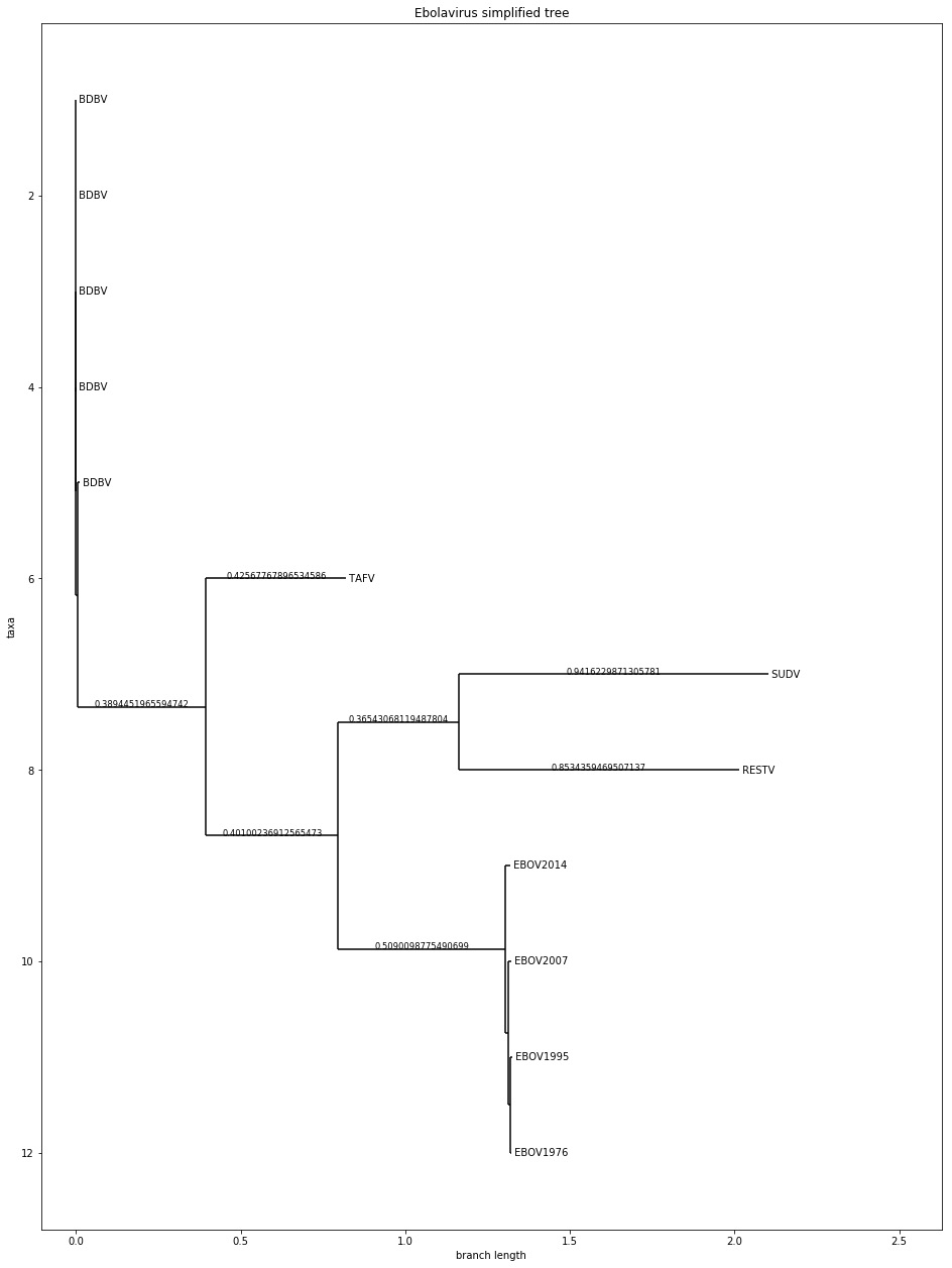
Figure 7.5 – A matplotlib-based version of the simplified dataset with branch lengths added

4. Now we will plot the complete dataset, but we will color each bit of the tree differently. If a subtree only has a single virus species, it will get its own color. EBOV will have two colors, that is, one for the 2014 outbreak and one for the others, as follows:

   fig = plt.figure(figsize=(16, 22))

   ax = fig.add_subplot(111)

   from collections import OrderedDict

   my_colors = OrderedDict({

   'EBOV_2014': 'red',

   'EBOV': 'magenta',

   'BDBV': 'cyan',

   'SUDV': 'blue',

   'RESTV' : 'green',

   'TAFV' : 'yellow'

   })

   def get_color(name):

       for pref, color in my_colors.items():

           if name.find(pref) > -1:

               return color

       return 'grey'

   def color_tree(node, fun_color=get_color):

       if node.is_terminal():

           node.color = fun_color(node.name)

       else:

           my_children = set()

           for child in node.clades:

               color_tree(child, fun_color)

               my_children.add(child.color.to_hex())

           if len(my_children) == 1:

               node.color = child.color

           else:

               node.color = 'grey'

   ebola_color_tree = deepcopy(ebola_tree)

   color_tree(ebola_color_tree.root)

   Phylo.draw(ebola_color_tree, axes=ax, label_func=lambda x: x.name.split(' ')[0][1:] if x.name is not None else None)

This is a tree traversing algorithm, not unlike the ones presented in the previous recipe. As a recursive algorithm, it works in the following way. If the node is a leaf, it will get a color based on its species (or the EBOV outbreak year). If it’s an internal node and all the descendant nodes below it are of the same species, it will get the color of that species; if there are several species after that, it will be colored in gray. Actually, the color function can be changed and will be changed later. Only the edge colors will be used (the labels will be printed in black).

Note that ladderization (performed in the previous recipe with DendroPy) helps quite a lot in terms of a clear visual appearance.

We also deep copy the genus tree to color a copy; remember from the previous recipe that some tree traversal functions can change the state, and in this case, we want to preserve a version without any coloring.

Note the usage of the lambda function to clean up the name that was changed by trimAl, as shown in the following diagram:

Figure 7.6 – A ladderized and colored phylogenetic tree with the complete Ebola virus dataset

There’s more...

Tree and graph visualization is a complex topic; arguably, here, the tree’s visualization is rigorous but far from pretty. One alternative to DendroPy, which has more visualization features, is ETE (http://etetoolkit.org/). General alternatives for drawing trees and graphs include Cytoscape (https://cytoscape.org/) and Gephi (http://gephi.github.io/). If you want to know more about the algorithms for rendering trees and graphs, check out the Wikipedia page at http://en.wikipedia.org/wiki/Graph_drawing for an introduction to this fascinating topic.

Be careful not to trade style for substance, though. For example, the previous edition of this book had a pretty rendering of a phylogenetic tree using a graph-rendering library. While it was clearly the most beautiful image in that chapter, it was misleading in terms of branch lengths.