11

Parallel Processing with Dask and Zarr

Bioinformatics datasets are growing at an exponential rate. Data analysis strategies based on standard tools such as Pandas assume that datasets are able to fit in memory (though with some provision for out-of-core analysis) or that a single machine is able to efficiently process all the data. This is, unfortunately, not realistic for many modern datasets.

In this chapter, we will introduce two libraries that are able to deal with very large datasets and expensive computations:

• Dask is a library that allows parallel computing that can scale from a single computer to very large cloud and cluster environments. Dask provides interfaces that are similar to Pandas and NumPy while allowing you to deal with large datasets spread over many computers.
• Zarr is a library that stores compressed and chunked multidimensional arrays. As we will see, these arrays are tailored to deal with very large datasets processed in large computer clusters, while still being able to process data on a single computer if need be.

Our recipes will introduce these advanced libraries using data from mosquito genomics. You should look at this code as a starting point to get you on the path to processing large datasets. Parallel processing of large datasets is a complex topic, and this is the beginning—not the end—of your journey.

Because all these libraries are fundamental for data analysis, if you are using Docker, they all can be found on the tiagoantao/bioinformatics_dask Docker image.

In this chapter, we will cover the following recipes:

• Reading genomics data with Zarr
• Parallel processing of data using Python multiprocessing
• Using Dask to process genomic data based on NumPy arrays
• Scheduling tasks with dask.distributed

Reading genomics data with Zarr

Zarr (https://zarr.readthedocs.io/en/stable/) stores array-based data—such as NumPy —in a hierarchical structure on disk and cloud storage. The data structures used by Zarr to represent arrays are not only very compact but also allow for parallel reading and writing, something we will see in the next recipes. In this recipe, we will be reading and processing genomics data from the Anopheles gambiae 1000 Genomes project (https://malariagen.github.io/vector-data/ag3/download.html). Here, we will simply do sequential processing to ease the introduction to Zarr; in the following recipe, we will do parallel processing. Our project will be computing the missingness for all genomic positions sequenced for a single chromosome.

Getting ready

The Anopheles 1000 Genomes data is available from Google Cloud Platform (GCP). To download data from GCP, you will need gsutil, available from https://cloud.google.com/storage/docs/gsutil_install. After you have gsutil installed, download the data (~2 gigabytes (GB)) with the following lines of code:

mkdir -p data/AG1000G-AO/

gsutil -m rsync -r

         -x '.*/calldata/(AD|GQ|MQ)/.*'

         gs://vo_agam_release/v3/snp_genotypes/all/AG1000G-AO/

         data/AG1000G-AO/ > /dev/null

We download a subset of samples from the project. After downloading the data, the code to process it can be found in Chapter11/Zarr_Intro.py.

How to do it...

Take a look at the following steps to get started:

1. Let’s start by checking the structure made available inside the Zarr file:

   import numpy as np

   import zarr

   mosquito = zarr.open('data/AG1000G-AO')

   print(mosquito.tree())

We start by opening the Zarr file (as we will soon see, this might not actually be a file). After that, we print the tree of data available inside it:

/

├── 2L

│   └── calldata

│       └── GT (48525747, 81, 2) int8

├── 2R

│   └── calldata

│       └── GT (60132453, 81, 2) int8

├── 3L

│   └── calldata

│       └── GT (40758473, 81, 2) int8

├── 3R

│   └── calldata

│       └── GT (52226568, 81, 2) int8

├── X

│   └── calldata

│       └── GT (23385349, 81, 2) int8

└── samples (81,) |S24

The Zarr file has five arrays: four correspond to chromosomes in the mosquito—2L, 2R, 3L, 3R, and X (Y is not included)—and one has a list of 81 samples included in the file. The last array has the sample names included—we have 81 samples in this file. The chromosome data is made of 8-bit integers (int8), and the sample names are strings.

2. Now, let’s explore the data for chromosome 2L. Let’s start with some basic information:

   gt_2l = mosquito['/2L/calldata/GT']

   gt_2l

Here is the output:

<zarr.core.Array '/2L/calldata/GT' (48525747, 81, 2) int8>

We have an array of 4852547 single-nucleotide polymorphisms (SNPs), for 81 samples. For each SNP and sample, we have 2 alleles.

3. Let’s now inspect how the data is stored:

   gt_2l.info

The output looks like this:

Name               : /2L/calldata/GT

Type               : zarr.core.Array

Data type          : int8

Shape              : (48525747, 81, 2)

Chunk shape        : (300000, 50, 2)

Order              : C

Read-only          : False

Compressor         : Blosc(cname='lz4', clevel=5, shuffle=SHUFFLE, blocksize=0)

Store type         : zarr.storage.DirectoryStore

No. bytes          : 7861171014 (7.3G)

No. bytes stored   : 446881559 (426.2M)

Storage ratio      : 17.6

Chunks initialized : 324/324

There is a lot to unpack here, but for now, we will concentrate on the store type, bytes stored, and storage ratio. The Store type value is zarr.storage.DirectoryStore, so the data is not in a single file but inside a directory. The raw size of the data is 7.3 GB! But Zarr uses a compressed format that reduces the size to 426.2 megabytes (MB). This means a compression ratio of 17.6.

4. Let’s peek at how the data is stored inside the directory. If you list the contents of the AG1000G-AO directory, you will find the following structure:

   .

   ├── 2L

   │   └── calldata

   │       └── GT

   ├── 2R

   │   └── calldata

   │       └── GT

   ├── 3L

   │   └── calldata

   │       └── GT

   ├── 3R

   │   └── calldata

   │       └── GT

   ├── samples

   └── X

       └── calldata

           └── GT

5. If you list the contents of 2L/calldata/GT, you will find plenty of files encoding the array:

   0.0.0

   0.1.0

   1.0.0

   ...

   160.0.0

   160.1.0

There are 324 files inside the 2L/calldata/GT directory. Remember from a previous step that we have a parameter called Chunk shape with a value of (300000, 50, 2).

Zarr splits the array into chunks—bits that are easier to process in memory than loading the whole array. Each chunk has 30000x50x2 elements. Given that we have 48525747 SNPs, we need 162 chunks to represent the number of SNPs (48525747/300000 = 161.75) and then multiply it by 2 for the number of samples (81 samples/50 per chunk = 1.62). Hence, we end up with 162*2 chunks/files.

Tip

Chunking is a technique widely used to deal with data that cannot be fully loaded into memory in a single pass. This includes many other libraries such as Pandas or Zarr. We will see an example with Zarr later. The larger point is that you should be aware of the concept of chunking as it is applied in many cases requiring big data.

6. Before we load the Zarr data for processing, let’s create a function to compute some basic genomic statistics for a chunk. We will compute missingness, the number of ancestral homozygotes, and the number of heterozygotes:

   def calc_stats(my_chunk):

       num_miss = np.sum(np.equal(my_chunk[:,:,0], -1), axis=1)

       num_anc_hom = np.sum(

           np.all([

               np.equal(my_chunk[:,:,0], 0),

               np.equal(my_chunk[:,:,0], my_chunk[:,:,1])], axis=0), axis=1)

       num_het = np.sum(

           np.not_equal(

               my_chunk[:,:,0],

               my_chunk[:,:,1]), axis=1)

       return num_miss, num_anc_hom, num_het

If you look at the previous function, you will notice that there is nothing Zarr-related: it’s just NumPy code. Zarr has a very light application programming interface (API) that exposes most of the data inside NumPy, making it quite easy to use if you know NumPy.

7. Finally, let’s traverse our data—that is, traverse our chunks to compute our statistics:

   complete_data = 0

   more_anc_hom = 0

   total_pos = 0

   for chunk_pos in range(ceil(max_pos / chunk_pos_size)):

       start_pos = chunk_pos * chunk_pos_size

       end_pos = min(max_pos + 1, (chunk_pos + 1) * chunk_pos_size)

       my_chunk = gt_2l[start_pos:end_pos, :, :]

       num_samples = my_chunk.shape[1]

       num_miss, num_anc_hom, num_het = calc_stats(my_chunk)

       chunk_complete_data = np.sum(np.equal(num_miss, 0))

       chunk_more_anc_hom = np.sum(num_anc_hom > num_het)

       complete_data += chunk_complete_data

       more_anc_hom += chunk_more_anc_hom

       total_pos += (end_pos - start_pos)

   print(complete_data, more_anc_hom, total_pos)

Most of the code takes care of the management of chunks and involves arithmetic to decide which part of the array to access. The important part in terms of ready Zarr data is the my_chunk = gt_2l[start_pos:end_pos, :, :] line. When you slice a Zarr array, it will automatically return a NumPy array.

Tip

Be very careful with the amount of data that you bring into memory. Remember that most Zarr arrays will be substantially bigger than the memory that you have available, so if you try to load it, your application and maybe even your computer will crash. For example, if you do all_data = gt_2l[:, :, :], you will need around 8 GB of free memory to load it—as we have seen earlier, the data is 7.3 GB in size.

There’s more...

Zarr has many more features than those presented here, and while we will explore some more in the next recipes, there are some possibilities that you should be aware of. For example, Zarr is one of the only libraries that allow for concurrent writing of data. You can also change the internal format of a Zarr representation.

As we have seen here, Zarr is able to compress data in very efficient ways—this is made possible by using the Blosc library (https://www.blosc.org/). You can change the internal compression algorithm of Zarr data owing to the flexibility of Blosc.

See also

There are alternative formats to Zarr—for example, Hierarchical Data Format 5 (HDF5) (https://en.wikipedia.org/wiki/Hierarchical_Data_Format) and Network Common Data Form (NetCDF) (https://en.wikipedia.org/wiki/NetCDF). While these are more common outside the bioinformatics space, they have less functionality—for example, a lack of concurrent writes.

Parallel processing of data using Python multiprocessing

When dealing with lots of data, one strategy is to process it in parallel so that we make use of all available central processing unit (CPU) power, given that modern machines have many cores. In a theoretical best-case scenario, if your machine has eight cores, you can get an eight-fold increase in performance if you do parallel processing.

Unfortunately, typical Python code only makes use of a single core. That being said, Python has built-in functionality to use all available CPU power; in fact, Python provides several avenues for that. In this recipe, we will be using the built-in multiprocessing module. The solution presented here works well in a single computer and if the dataset fits into memory, but if you want to scale it in a cluster or the cloud, you should consider Dask, which we will introduce in the next two recipes.

Our objective here will again be to compute some statistics around missingness and heterozygosity.

Getting ready

We will be using the same data as in the previous recipe. The code for this recipe can be found in Chapter11/MP_Intro.py.

How to do it...

Follow these steps to get started:

1. We will be using the exact same function as in the previous recipe to calculate statistics—this is heavily NumPy-based:

   import numpy as np

   import zarr

   def calc_stats(my_chunk):

       num_miss = np.sum(np.equal(my_chunk[:,:,0], -1), axis=1)

       num_anc_hom = np.sum(

           np.all([

               np.equal(my_chunk[:,:,0], 0),

               np.equal(my_chunk[:,:,0], my_chunk[:,:,1])], axis=0), axis=1)

       num_het = np.sum(

           np.not_equal(

               my_chunk[:,:,0],

               my_chunk[:,:,1]), axis=1)

       return num_miss, num_anc_hom, num_het

2. Let’s access our mosquito data:

   mosquito = zarr.open('data/AG1000G-AO')

   gt_2l = mosquito['/2L/calldata/GT']

3. While we are using the same function to calculate statistics, our approach will be different for the whole dataset. First, we compute all the intervals for which we will call calc_stats. The intervals will be devised to match perfectly with the chunk division for variants:

   chunk_pos_size = gt_2l.chunks[0]

   max_pos = gt_2l.shape[0]

   intervals = []

   for chunk_pos in range(ceil(max_pos / chunk_pos_size)):

       start_pos = chunk_pos * chunk_pos_size

       end_pos = min(max_pos + 1, (chunk_pos + 1) * chunk_pos_size)

       intervals.append((start_pos, end_pos))

It is important that our interval list is related to the chunking on disk. The computation will be efficient as long as this mapping is as close as possible.

4. We are now going to separate the code to compute each interval in a function. This is important as the multiprocessing module will execute this function many times on each process that it creates:

   def compute_interval(interval):

       start_pos, end_pos = interval

       my_chunk = gt_2l[start_pos:end_pos, :, :]

       num_samples = my_chunk.shape[1]

       num_miss, num_anc_hom, num_het = calc_stats(my_chunk)

       chunk_complete_data = np.sum(np.equal(num_miss, 0))

       chunk_more_anc_hom = np.sum(num_anc_hom > num_het)

       return chunk_complete_data, chunk_more_anc_hom

5. We are now finally going to execute our code over several cores:

   with Pool() as p:

       print(p)

       chunk_returns = p.map(compute_interval, intervals)

       complete_data = sum(map(lambda x: x[0], chunk_returns))

       more_anc_hom = sum(map(lambda x: x[1], chunk_returns))

       print(complete_data, more_anc_hom)

The first line creates a context manager using the multiprocessing.Pool object. The Pool object, by default, creates several processes numbered os.cpu_count(). The pool provides a map function that will call our compute_interval function across all processes created. Each call will take one of the intervals.

There’s more...

This recipe provides a small introduction to parallel processing with Python without the need to use external libraries. That being said, it presents the most important building block for concurrent parallel processing with Python.

Due to the way thread management is implemented in Python, threading is not a viable alternative for real parallel processing. Pure Python code cannot be run in parallel using multithreading.

Some libraries that you might use—and this is normally the case with NumPy—are able to make use of all underlying processors even when executing a sequential piece of code. Make sure that when making use of external libraries, you are not overcommitting processor resources: this happens when you have multiple processes, and underlying libraries also make use of many cores.

See also

• There is way more to be discussed about the multiprocessing module. You can start with the standard documentation at https://docs.python.org/3/library/multiprocessing.html.
• To understand why Python-based multithreading doesn’t make use of all CPU resources, read about the Global Interpreter Lock (GIL) at https://realpython.com/python-gil/.

Using Dask to process genomic data based on NumPy arrays

Dask is a library that provides advanced parallelism that can scale from a single computer to very large clusters or a cloud operation. It also provides the ability to process datasets that are larger than memory. It is able to provide interfaces that are similar to common Python libraries such as NumPy, Pandas, or scikit-learn.

We are going to repeat a subset of the example from previous recipes—namely, compute missingness for the SNPs in our dataset. We will be using an interface similar to NumPy that is offered by Dask.

Before we start, be aware that the semantics of Dask are quite different from libraries such as NumPy or Pandas: it is a lazy library. For example, when you specify a call equivalent to—say—np.sum, you are not actually calculating a sum, but adding a task that in the future will eventually calculate it. Let’s get into the recipe to make things clearer.

Getting ready

We are going to rechunk the Zarr data in a completely different way. The reason we do that is so that we can visualize task graphs during the preparation of our algorithm. Task graphs with five operations are easier to visualize than task graphs with hundreds of nodes. For practical purposes, you should not rechunk in so little chunks as we do here. In fact, you will be perfectly fine if you don’t rechunk this dataset at all. We are only doing it for visualization purposes:

import zarr
mosquito = zarr.open('data/AG1000G-AO/2L/calldata/GT')
zarr.array(
    mosquito,
    chunks=(1 + 48525747 // 4, 81, 2),
    store='data/rechunk')

We will end up with very large chunks, and while that is good for our visualization purpose, they might be too big to fit in memory.

The code for this recipe can be found in Chapter11/Dask_Intro.py.

How to do it...

1. Let’s first load the data and inspect the size of the DataFrame:

   import numpy as np

   import dask.array as da

   mosquito = da.from_zarr('data/rechunk')

   mosquito

Here is the output if you are executing inside Jupyter:

Figure 11.1 - Jupyter output for a Dask array, summarizing our data

The full array takes up 7.32 GB. The most important number is the chunk size: 1.83 GB. Each worker will need to have enough memory to process a chunk. Remember that we are only using such a smaller number of chunks to be able to plot the tasks here.

Because of the large chunk sizes, we end up with just four chunks.

We did not load anything in memory yet: we just specified that we want to eventually do it. We are creating a task graph to be executed, not executing—at least for now.

2. Let’s see which tasks we have to execute to load the data:

   mosquito.visualize()

Here is the output:

Figure 11.2 - Tasks that need to be executed to load our Zarr array

We thus have four tasks to execute, one for each chunk.

3. Now, let’s look at the function to compute missingness per chunk:

   def calc_stats(variant):

       variant = variant.reshape(variant.shape[0] // 2, 2)

       misses = np.equal(variant, -1)

       return misses

The function per chunk will operate on NumPy arrays. Note the difference: the code that we use to work on the main loop works with Dask arrays, but at the chunk level the data is presented as a NumPy array. Hence, the chunks have to fit in memory as NumPy requires that.

4. Later, when we actually use the function, we need to have a two-dimensional (2D) array. Given that the array is three-dimensional (3D), we will need to reshape the array:

   mosquito_2d = mosquito.reshape(

       mosquito.shape[0],

       mosquito.shape[1] * mosquito.shape[2])

   mosquito_2d.visualize()

Here is the task graph as it currently stands:

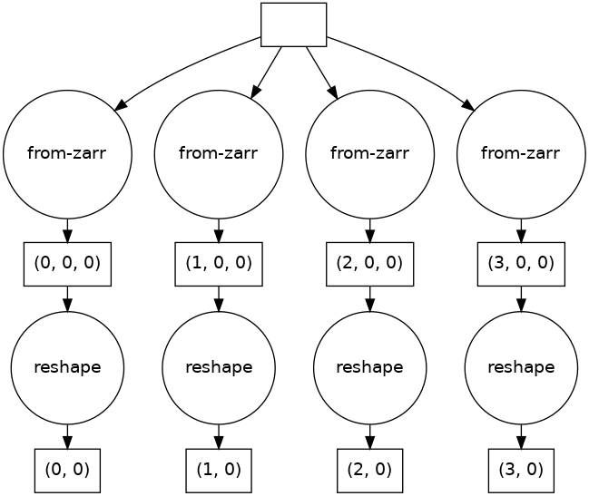
Figure 11.3 - The task graph to load genomic data and reshape it

The reshape operation is happening at the dask.array level, not at the NumPy level, so it just added nodes to the task graph. There is still no execution.

5. Let’s now prepare to execute the function—meaning adding tasks to our task graph—over all our dataset. There are many ways to execute it; here, we are going to use the apply_along_axis function that dask.array provides and is based on the equally named function from NumPy:

   max_pos = 10000000

   stats = da.apply_along_axis(

       calc_stats, 1, mosquito_2d[:max_pos,:],

       shape=(max_pos,), dtype=np.int64)

   stats.visualize()

For now, we are only going to study the first million positions. As you can see in the task graph, Dask is smart enough to only add an operation to the chunk involved in the computation:

Figure 11.4 - The complete task graph including statistical computing

6. Remember that we haven’t computed anything until now. It is now time to actually execute the task graph:

   stats = stats.compute()

This will start the computation. Precisely how the computation is done is something we will discuss in the next recipe.

WARNING

Because of the chunk size, this code might crash your computer. You will be safe with at least 16 GB of memory. Remember that you can use smaller chunk sizes—and you should use smaller chunk sizes. We just used chunk sizes like this in order to be able to generate the task graphs shown earlier (if not, they would have possibly hundreds of nodes and would be unprintable).

There’s more...

We didn’t spend any time here discussing strategies to optimize the code for Dask—that would be a book of its own. For very complex algorithms, you will need to research further into the best practices.

Dask provides interfaces similar to other known Python libraries such as Pandas or scikit-learn that can be used for parallel processing. You can also use it for general algorithms that are not based on existing libraries.

See also

• For best practices with Dask, your best starting point is the Dask documentation itself, especially https://docs.dask.org/en/latest/best-practices.html.

Scheduling tasks with dask.distributed

Dask is extremely flexible in terms of execution: we can execute locally, on a scientific cluster, or on the cloud. That flexibility comes at a cost: it needs to be parameterized. There are several alternatives to configure a Dask schedule and execution, but the most generic is dask.distributed as it is able to manage different kinds of infrastructure. Because I cannot assume you have access to a cluster or a cloud such as Amazon Web Services (AWS) or GCP, we will be setting up computation on your local machine, but remember that you can set up dask.distributed on very different kinds of platforms.

Here, we will again compute simple statistics over variants of the Anopheles 1000 Genomes project.

Getting ready

Before we start with dask.distributed, we should note that Dask has a default scheduler that actually can change depending on the library you are targeting. For example, here is the scheduler for our NumPy example:

import dask
from dask.base import get_scheduler
import dask.array as da
mosquito = da.from_zarr('data/AG1000G-AO/2L/calldata/GT')
print(get_scheduler(collections=[mosquito]).__module__)

The output will be as follows:

dask.threaded

Dask uses a threaded scheduler here. This makes sense for a NumPy array: NumPy implementation is itself multithreaded (real multithreaded with parallelism). We don’t want lots of processes running when the underlying library is running in parallel to itself. If you had a Pandas DataFrame, Dask would probably choose a multiprocessor scheduler. As Pandas is not parallel, it makes sense for Dask to run in parallel itself.

OK—now that we have that important detail out of the way, let’s get back to preparing our environment.

dask.distributed has a centralized scheduler and a set of workers, and we need to start those. Run this code in the command line to start the scheduler:

dask-scheduler --port 8786 --dashboard-address 8787

We can start workers on the same machine as the scheduler, like this:

dask-worker --nprocs 2 –nthreads 1 127.0.0.1:8786

I specified two processes with a single thread per process. This is reasonable for NumPy code, but the actual configuration will depend on your workload (and be completely different if you are on a cluster or a cloud).

Tip

You actually do not need to start the whole process manually as I did here. dask.distributed will start something for you—not really optimized for your workload—if you don’t prepare the system yourself (see the following section for details). But I wanted to give you a flavor of the effort as in many cases, you will have to set up the infrastructure yourself.

Again, we will be using data from the first recipe. Be sure you download and prepare it, as explained in its Getting ready section. We won’t be using the rechunked part—we will be doing it in our Dask code in the following section. Our code is available in Chapter11/Dask_distributed.py.

How to do it...

Follow these steps to get started:

1. Let’s start by connecting to the scheduler that we created earlier:

   import numpy as np

   import zarr

   import dask.array as da

   from dask.distributed import Client

   client = Client('127.0.0.1:8786')

   client

If you are on Jupyter, you will get a nice output summarizing the configuration you created in the Getting ready part of this recipe:

Figure 11.5 - Summary of your execution environment with dask.distributed

You will notice the reference to a dashboard here. dask.distributed provides a real-time dashboard over the web that allows you to track the state of the computation. Point your browser to http://127.0.0.1:8787/ to find it, or just follow the link provided in Figure 11.5.

As we still haven’t done any computations, the dashboard is mostly empty. Be sure to explore the many tabs along the top:

Figure 11.6 - The starting state of the dask.distributed dashboard

2. Let’s load the data. More rigorously, let’s prepare the task graph to load the data:

   mosquito = da.from_zarr('data/AG1000G-AO/2L/calldata/GT')

   mosquito

Here is the output on Jupyter:

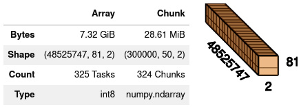
Figure 11.7 - Summary of the original Zarr array for chromosome 2L

3. To facilitate visualization, let’s rechunk again. We are also going to have a single chunk for the second dimension, which is the samples. This is because our computation of missingness requires all the samples, and it makes little sense—in our specific case—to have two chunks per sample:

   mosquito = mosquito.rechunk((mosquito.shape[0]//8, 81, 2))

As a reminder, we have very large chunks, and you might end up with memory problems. If that is the case, then you can run it with the original chunks. It’s just that the visualization will be unreadable.

4. Before we continue, let’s ask Dask to not only execute the rechunking but also to have the results of it at the ready in the workers:

   mosquito = mosquito.persist()

The persist call makes sure the data is available in the workers. In the following screenshot, you can find the dashboard somewhere in the middle of the computation. You can find which tasks are executing on each node, a summary of tasks done and to be done, and the bytes stored per worker. Of note is the concept of spilled to disk (see the top left of the screen). If there is not enough memory for all chunks, they will temporarily be written to disk:

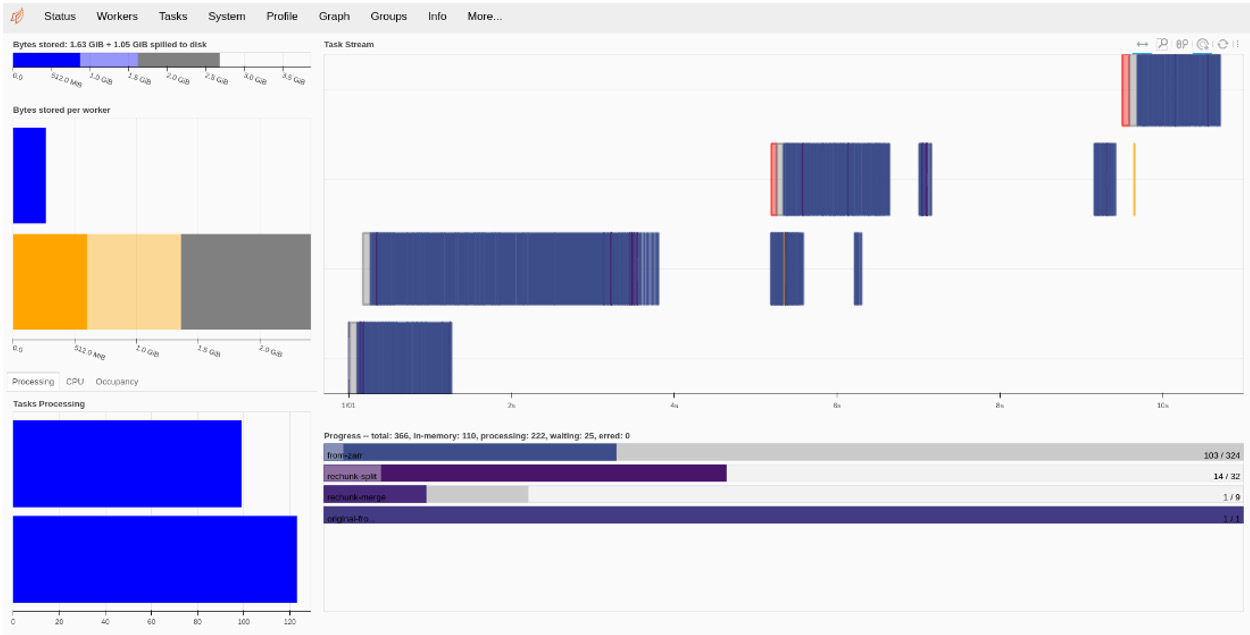
Figure 11.8 - The dashboard state while executing the persist function for rechunking the array

5. Let’s now compute the statistics. We will use a different approach for the last recipe—we will ask Dask to apply a function to each chunk:

   def calc_stats(my_chunk):

       num_miss = np.sum(

           np.equal(my_chunk[0][0][:,:,0], -1),

           axis=1)

       return num_miss

   stats = da.blockwise(

       calc_stats, 'i', mosquito, 'ijk',

       dtype=np.uint8)

   stats.visualize()

Remember that each chunk is not a dask.array instance but a NumPy array, so the code works on NumPy arrays. Here is the current task graph. There are no operations to load the data, as the function performed earlier executed all of those:

Figure 11.9 - Calls to the calc_stats function over chunks starting with persisted data

6. Finally, we can get our results:

   stat_results = stats.compute()

There’s more...

There is substantially more that can be said about the dask.distributed interface. Here, we introduced the basic concepts of its architecture and the dashboard.

dask.distributed provides an asynchronous interface based on the standard async module of Python. Due to the introductory nature of this chapter, we won’t address it, but you are recommended to look at it.

See also

• You can start with the documentation of dask.distributed at https://distributed.dask.org/en/stable/.
• In many cases, you will need to deploy your code in a cluster or the cloud. Check out the deployment documentation for resources on different platforms: https://docs.dask.org/en/latest/deploying.html.
• After you have mastered the content here, studying asynchronous computation in Python would be your next step. Check out https://docs.python.org/3/library/asyncio-task.html.