4

Advanced NGS Data Processing

If you work with next-generation sequencing (NGS) data, you know that quality analysis and processing are two of the great time-sinks in getting results. In the first part of this chapter, we will delve deeper into NGS analysis by using a dataset that includes information about relatives – in our case, a mother, a father, and around 20 offspring. This is a common technique for performing quality analysis, as pedigree information will allow us to make inferences on the number of errors that our filtering rules might produce. We will also take the opportunity to use the same dataset to find genomic features based on existing annotations.

The last recipe of this chapter will delve into another advanced topic using NGS data: metagenomics. We will QIIME2, a Python package for metagenomics, to analyze data.

If you are using Docker, please use the tiagoantao/bioinformatics_base image. The QIIME2 content has a special setup process that will be discussed in the relevant recipe.

In this chapter, there are the following recipes:

• Preparing a dataset for analysis
• Using Mendelian error information for quality control
• Exploring data with standard statistics
• Finding genomic features from sequencing annotations
• Doing metagenomics with QIIME2

Preparing a dataset for analysis

Our starting point will be a VCF file (or equivalent) with calls made by a genotyper (Genome Analysis Toolkit (GATK) in our case), including annotations. As we will be filtering NGS data, we need reliable decision criteria to call a site. So, how do we get that information? Generally, we can’t, but if we need to do so, there are three basic approaches:

• Using a more robust sequencing technology for comparison – for example, using Sanger sequencing to verify NGS datasets. This is cost-prohibitive and can only be done for a few loci.
• Sequencing closely related individuals, for example, two parents and their offspring. In this case, we use Mendelian inheritance rules to decide whether a certain call is acceptable or not. This was the strategy used by both the Human Genome Project and the Anopheles gambiae 1000 Genomes project.
• Finally, we can use simulations. This setup is not only quite complex but also of dubious reliability. It’s more of a theoretical option.

In this chapter, we will use the second option, based on the Anopheles gambiae 1000 Genomes project. This project makes available information based on crosses between mosquitoes. A cross will include the parents (mother and father) and up to 20 offspring.

In this recipe, we are going to prepare our data for usage in the later recipes.

Getting ready

We will download our files in HDF5 format for faster processing. Please be advised that these files are quite big; you will need a good network connection and plenty of disk space:

wget -c ftp://ngs.sanger.ac.uk/production/ag1000g/phase1/AR3/variation/main/hdf5/ag1000g.phase1.ar3.pass.3L.h5

wget -c ftp://ngs.sanger.ac.uk/production/ag1000g/phase1/AR3/variation/main/hdf5/ag1000g.phase1.ar3.pass.2L.h5

The files have four crosses with around 20 offspring each. We will use chromosome arms 3L and 2L. At this stage, we also compute Mendelian errors (a subject of the next recipe, so we will delay a detailed discussion until then).

The relevant notebook is Chapter04/Preparation.py. There is also a local sample metadata file in the directory called samples.tsv.

How to do it…

After downloading the data, follow these steps:

1. First, start with a few imports:

   import pickle

   import gzip

   import random

   import numpy as np

   import h5py

   import pandas as pd

2. Let’s get the sample metadata:

   samples = pd.read_csv('samples.tsv', sep=' ')

   print(len(samples))

   print(samples['cross'].unique())

   print(samples[samples['cross'] == 'cross-29-2'][['id', 'function']])

   print(len(samples[samples['cross'] == 'cross-29-2']))

   print(samples[samples['function'] == 'parent'])

We also print some basic information about the cross we are going to use and all the parents.

3. We prepare to deal with chromosome arm 3L based on its HDF5 file:

   h5_3L = h5py.File('ag1000g.crosses.phase1.ar3sites.3L.h5', 'r')

   samples_hdf5 = list(map(lambda sample: sample.decode('utf-8'), h5_3L['/3L/samples']))

   calldata_genotype = h5_3L['/3L/calldata/genotype']

   MQ0 = h5_3L['/3L/variants/MQ0']

   MQ = h5_3L['/3L/variants/MQ']

   QD = h5_3L['/3L/variants/QD']

   Coverage = h5_3L['/3L/variants/Coverage']

   CoverageMQ0 = h5_3L['/3L/variants/CoverageMQ0']

   HaplotypeScore = h5_3L['/3L/variants/HaplotypeScore']

   QUAL = h5_3L['/3L/variants/QUAL']

   FS = h5_3L['/3L/variants/FS']

   DP = h5_3L['/3L/variants/DP']

   HRun = h5_3L['/3L/variants/HRun']

   ReadPosRankSum = h5_3L['/3L/variants/ReadPosRankSum']

   my_features = {

       'MQ': MQ,

       'QD': QD,

       'Coverage': Coverage,

       'HaplotypeScore': HaplotypeScore,

       'QUAL': QUAL,

       'FS': FS,

       'DP': DP,

       'HRun': HRun,

       'ReadPosRankSum': ReadPosRankSum

   }

   num_features = len(my_features)

   num_alleles = h5_3L['/3L/variants/num_alleles']

   is_snp = h5_3L['/3L/variants/is_snp']

   POS = h5_3L['/3L/variants/POS']

4. The code to compute Mendelian errors is the following:

   #compute mendelian errors (biallelic)

   def compute_mendelian_errors(mother, father, offspring):

       num_errors = 0

       num_ofs_problems = 0

       if len(mother.union(father)) == 1:

           # Mother and father are homogenous and the            same for ofs in offspring:

               if len(ofs) == 2:

                   # Offspring is het

                   num_errors += 1

                   num_ofs_problems += 1

               elif len(ofs.intersection(mother)) == 0:

                   # Offspring is homo, but opposite from parents

                   num_errors += 2

                   num_ofs_problems += 1

       elif len(mother) == 1 and len(father) == 1:

           # Mother and father are homo and different

           for ofs in offspring:

               if len(ofs) == 1:

                   # Homo, should be het

                   num_errors += 1

                   num_ofs_problems += 1

       elif len(mother) == 2 and len(father) == 2:

           # Both are het, individual offspring can be anything

           pass

       else:

           # One is het, the other is homo

           homo = mother if len(mother) == 1 else father

           for ofs in offspring:

               if len(ofs) == 1 and ofs.intersection(homo):

                   # homo, but not including the allele from parent that is homo

                   num_errors += 1

                   num_ofs_problems += 1

       return num_errors, num_ofs_problems

We will discuss this in the next recipe, Using Mendelian error information for quality control.

5. We now define a support generator and function to select acceptable positions and accumulate basic data:

   def acceptable_position_to_genotype():

       for i, genotype in enumerate(calldata_genotype):

           if is_snp[i] and num_alleles[i] == 2:

               if len(np.where(genotype == -1)[0]) > 1:

                   # Missing data

                   continue

               yield i

   def acumulate(fun):

       acumulator = {}

       for res in fun():

           if res is not None:

               acumulator[res[0]] = res[1]

       return acumulator

6. We now need to find the indexes of our cross (mother, father, and 20 offspring) on the HDF5 file:

   def get_family_indexes(samples_hdf5, cross_pd):

       offspring = []

       for i, individual in cross_pd.T.iteritems():

           index = samples_hdf5.index(individual.id)

           if individual.function == 'parent':

               if individual.sex == 'M':

                   father = index

               else:

                   mother = index

           else:

               offspring.append(index)

       return {'mother': mother, 'father': father, 'offspring': offspring}

   cross_pd = samples[samples['cross'] == 'cross-29-2']

   family_indexes = get_family_indexes(samples_hdf5, cross_pd)

7. Finally, we will actually compute Mendelian errors and save them to disk:

   mother_index = family_indexes['mother']

   father_index = family_indexes['father']

   offspring_indexes = family_indexes['offspring']

   all_errors = {}

   def get_mendelian_errors():

       for i in acceptable_position_to_genotype():

           genotype = calldata_genotype[i]

           mother = set(genotype[mother_index])

           father = set(genotype[father_index])

           offspring = [set(genotype[ofs_index]) for ofs_index in offspring_indexes]

           my_mendelian_errors = compute_mendelian_errors(mother, father, offspring)

           yield POS[i], my_mendelian_errors

   mendelian_errors = acumulate(get_mendelian_errors)

   pickle.dump(mendelian_errors, gzip.open('mendelian_errors.pickle.gz', 'wb'))

8. We will now generate an efficient NumPy array with annotations and Mendelian error information:

   ordered_positions = sorted(mendelian_errors.keys())

   ordered_features = sorted(my_features.keys())

   num_features = len(ordered_features)

   feature_fit = np.empty((len(ordered_positions), len(my_features) + 2), dtype=float)

   for column, feature in enumerate(ordered_features):  # 'Strange' order

       print(feature)

       current_hdf_row = 0

       for row, genomic_position in enumerate(ordered_positions):

           while POS[current_hdf_row] < genomic_position:

               current_hdf_row +=1

           feature_fit[row, column] = my_features[feature][current_hdf_row]

   for row, genomic_position in enumerate(ordered_positions):

       feature_fit[row, num_features] = genomic_position

       feature_fit[row, num_features + 1] = 1 if mendelian_errors[genomic_position][0] > 0 else 0

   np.save(gzip.open('feature_fit.npy.gz', 'wb'), feature_fit, allow_pickle=False, fix_imports=False)

   pickle.dump(ordered_features, open('ordered_features', 'wb'))

Buried in this code is one of the most important decisions of the whole chapter: how do we weigh Mendelian errors? In our case, we only store a 1 if there is any kind of error, and we store a 0 if there is none. An alternative would be to count the number of errors – as we have up to 20 offspring, that would require some sophisticated statistical analysis that we will not be doing here.

9. Changing gears, let’s extract some information from chromosome arm 2L now:

   h5_2L = h5py.File('ag1000g.crosses.phase1.ar3sites.2L.h5', 'r')

   samples_hdf5 = list(map(lambda sample: sample.decode('utf-8'), h5_2L['/2L/samples']))

   calldata_DP = h5_2L['/2L/calldata/DP']

   POS = h5_2L['/2L/variants/POS']

10. Here, we are only interested in the parents:

    def get_parent_indexes(samples_hdf5, parents_pd):

        parents = []

        for i, individual in parents_pd.T.iteritems():

            index = samples_hdf5.index(individual.id)

            parents.append(index)

        return parents

    parents_pd = samples[samples['function'] == 'parent']

    parent_indexes = get_parent_indexes(samples_hdf5, parents_pd)

11. We extract the sample DP for each parent:

    all_dps = []

    for i, pos in enumerate(POS):

        if random.random() > 0.01:

            continue

        pos_dp = calldata_DP[i]

        parent_pos_dp = [pos_dp[parent_index] for parent_index in parent_indexes]

        all_dps.append(parent_pos_dp + [pos])

    all_dps = np.array(all_dps)

    np.save(gzip.open('DP_2L.npy.gz', 'wb'), all_dps, allow_pickle=False, fix_imports=False)

Now, we have prepared the dataset for analysis in this chapter.

Using Mendelian error information for quality control

So, how can we infer the quality of calls using Mendelian inheritance rules? Let’s look at expectations for different genotypical configurations of the parents:

• For a certain potential bi-allelic SNP, if the mother is AA and the father is also AA, then all offspring will be AA.
• If the mother is AA and the father TT, then all offspring will have to be heterozygous (AT). They always get an A from the mother, and they always get a T from the father.
• If the mother is AA and the father is AT, then the offspring can be either AA or AT. They always get an A from the mother, but they can get either an A or a T from the father.
• If both the mother and the father are heterozygous (AT), then the offspring can be anything. In theory, there is not much we can do here.

In practice, we can ignore mutations, which is safe to do with most eukaryotes. The number of mutations (noise, from our perspective) is several orders of magnitude lower than the signal we are looking for.

In this recipe, we are going to do a small theoretical study of the distribution and Mendelian errors, and further process the data for downstream analysis based on errors. The relevant notebook file is Chapter04/Mendel.py.

How to do it…

1. We will need a few imports:

   import random

   import matplotlib.pyplot as plt

2. Before we do any empirical analysis, let’s try to understand what information we can extract from the case where the mother is AA and the father is AT. Let’s answer the question, If we have 20 offspring, what is the probability of all of them being heterozygous?:

   num_sims = 100000

   num_ofs = 20

   num_hets_AA_AT = []

   for sim in range(num_sims):

       sim_hets = 0

       for ofs in range(20):

           sim_hets += 1 if random.choice([0, 1]) == 1 else 0

       num_hets_AA_AT.append(sim_hets)

       

   fig, ax = plt.subplots(1,1, figsize=(16,9))

   ax.hist(num_hets_AA_AT, bins=range(20))

   print(len([num_hets for num_hets in num_hets_AA_AT if num_hets==20]))

We get the following output:

Figure 4.1 - Results from 100,000 simulations: the number of offspring that are heterozygous for certain loci where the mother is AA and the father is heterozygous

Here, we have done 100,000 simulations. In my case (this is stochastic, so your result might vary), I got exactly zero simulations where all offspring were heterozygous. Indeed, these are permutations with repetition, so the probability of all being heterozygous is or 9.5367431640625e-07 – not very likely. So, even if for a single offspring, we can have AT or AA; for 20, it is very unlikely that all of them are of the same type. This is the information we can use for a less naive interpretation of Mendelian errors.

3. Let’s repeat the analysis where the mother and the father are both AT:

   num_AAs_AT_AT = []

   num_hets_AT_AT = []

   for sim in range(num_sims):

       sim_AAs = 0

       sim_hets = 0

       for ofs in range(20):

           derived_cnt = sum(random.choices([0, 1], k=2))

           sim_AAs += 1 if derived_cnt == 0 else 0

           sim_hets += 1 if derived_cnt == 1 else 0

       num_AAs_AT_AT.append(sim_AAs)

       num_hets_AT_AT.append(sim_hets)

   fig, ax = plt.subplots(1,1, figsize=(16,9))

   ax.hist([num_hets_AT_AT, num_AAs_AT_AT], histtype='step', fill=False, bins=range(20), label=['het', 'AA'])

   plt.legend()

The output is as follows:

Figure 4.2 - Results from 100,000 simulations: the number of offspring that are AA or heterozygous for a certain locus where both parents are also heterozygous

In this case, we have also permutations with repetition, but we have four possible values, not two: AA, AT, TA, and TT. We end up with the same probability for all individuals being AT: 9.5367431640625e-07. It’s even worse (twice as bad, in fact) for all of them being homozygous of the same type (all TT or all AA).

4. OK, after this probabilistic prelude, let’s get down to more data-moving stuff. The first thing that we will do is check how many errors we have. Let’s load the data from the previous recipe:

   import gzip

   import pickle

   import random

   import numpy as np

   mendelian_errors = pickle.load(gzip.open('mendelian_errors.pickle.gz', 'rb'))

   feature_fit = np.load(gzip.open('feature_fit.npy.gz', 'rb'))

   ordered_features = np.load(open('ordered_features', 'rb'))

   num_features = len(ordered_features)

5. Let’s see how many errors we have:

   print(len(mendelian_errors), len(list(filter(lambda x: x[0] > 0,mendelian_errors.values()))))

The output is as follows:

(10905732, 541688)

Not many of the calls have Mendelian errors – only around 5%, great.

6. Let’s create a balanced set where roughly half of the set has errors. For that, we will randomly drop a lot of good calls. First, we compute the fraction of errors:

   total_observations = len(mendelian_errors)

   error_observations = len(list(filter(lambda x: x[0] > 0,mendelian_errors.values())))

   ok_observations = total_observations - error_observations

   fraction_errors = error_observations/total_observations

   print (total_observations, ok_observations, error_observations, 100*fraction_errors)

   del mendelian_errors

7. We use that information to get a set of accepted entries: all the errors plus an approximately equal quantity of OK calls. We print the number of entries at the end (this will vary as the OK list is stochastic):

   prob_ok_choice = error_observations / ok_observations

   def accept_entry(row):

       if row[-1] == 1:

           return True

       return random.random() <= prob_ok_choice

   accept_entry_v = np.vectorize(accept_entry, signature='(i)->()')

   accepted_entries = accept_entry_v(feature_fit)

   balanced_fit = feature_fit[accepted_entries]

   del feature_fit

   balanced_fit.shape

   len([x for x in balanced_fit if x[-1] == 1]), len([x for x in balanced_fit if x[-1] == 0])

8. Finally, we save it:

   np.save(gzip.open('balanced_fit.npy.gz', 'wb'), balanced_fit, allow_pickle=False, fix_imports=False)

There’s more…

With regards to Mendelian errors and their impact on cost functions, let’s think about the following case: the mother is AA, the father is AT, and all offspring are AA. Does this mean that the father is wrongly called, or that we failed to detect a few heterozygous offspring? From this reasoning, it’s probably the father that is wrongly called. This has an impact in terms of some more refined Mendelian error estimation functions: it’s probably more costly to have a few offspring wrong than just a single sample (the father) wrong. In this case, you might think it’s trivial (the probability of having no heterozygous offspring is so low that it’s probably the father), but if you have 18 offspring AA and two AT, is it still “trivial”? This is not just a theoretical problem, because it severely impacts the design of a proper cost function.

Our function in a previous recipe, Preparing the dataset for analysis, is naive but is enough for the level of refinement that will allow us to have some interesting results further down the road.

Exploring the data with standard statistics

Now that we have the insights for our Mendelian error analysis, let’s explore the data in order to get more insights that might help us to better filter the data. You can find this content in Chapter04/Exploration.py.

How to do it…

1. We start, as usual, with the necessary imports:

   import gzip

   import pickle

   import random

   import numpy as np

   import matplotlib.pyplot as plt

   import pandas as pd

   from pandas.plotting import scatter_matrix

2. Then we load the data. We will use pandas to navigate it:

   fit = np.load(gzip.open('balanced_fit.npy.gz', 'rb'))

   ordered_features = np.load(open('ordered_features', 'rb'))

   num_features = len(ordered_features)

   fit_df = pd.DataFrame(fit, columns=ordered_features + ['pos', 'error'])

   num_samples = 80

   del fit

3. Let’s ask pandas to show a histogram of all annotations:

   fig,ax = plt.subplots(figsize=(16,9))

   fit_df.hist(column=ordered_features, ax=ax)

The following histogram is generated:

Figure 4.3 - Histogram of all annotations for a dataset with roughly 50% of errors

4. For some annotations, we do not get interesting information. We can try to zoom in, for example, with DP:

   fit_df['MeanDP'] = fit_df['DP'] / 80

   fig, ax = plt.subplots()

   _ = ax.hist(fit_df[fit_df['MeanDP']<50]['MeanDP'], bins=100)

Figure 4.4 - Histogram zooming in on an area of interest for DP

We are actually dividing DP by the number of samples in order to get a more meaningful number.

5. We will split the dataset in two, one for the errors and the other for the positions with no Mendelian errors:

   errors_df = fit_df[fit_df['error'] == 1]

   ok_df = fit_df[fit_df['error'] == 0]

6. Let’s have a look at QUAL and split it on 0.005, and check how we get errors and correct calls split:

   ok_qual_above_df = ok_df[ok_df['QUAL']>0.005]

   errors_qual_above_df = errors_df[errors_df['QUAL']>0.005]

   print(ok_df.size, errors_df.size, ok_qual_above_df.size, errors_qual_above_df.size)

   print(ok_qual_above_df.size / ok_df.size, errors_qual_above_df.size / errors_df.size)

The result is as follows:

6507972 6500256 484932 6114096

0.07451353509203788 0.9405931089483245

Clearly, ['QUAL']>0.005 gets lots of errors, while not getting lots of OK positions. This is positive, as we have some hope for filtering it.

7. Let’s do the same with QD:

   ok_qd_above_df = ok_df[ok_df['QD']>0.05]

   errors_qd_above_df = errors_df[errors_df['QD']>0.05]

   print(ok_df.size, errors_df.size, ok_qd_above_df.size, errors_qd_above_df.size)

   print(ok_qd_above_df.size / ok_df.size, errors_qd_above_df.size / errors_df.size)

Again, we have some interesting results:

6507972 6500256 460296 5760288

0.07072802402960554 0.8861632526472804

8. Let’s take an area where there are fewer errors and study the relationships between annotations on errors. We will plot annotations pairwise:

   not_bad_area_errors_df = errors_df[(errors_df['QUAL']<0.005)&(errors_df['QD']<0.05)]

   _ = scatter_matrix(not_bad_area_errors_df[['FS', 'ReadPosRankSum', 'MQ', 'HRun']], diagonal='kde', figsize=(16, 9), alpha=0.02)

The preceding code generates the following output:

Figure 4.5 - Scatter matrix of annotations of errors for an area of the search space

9. And now do the same on the good calls:

   not_bad_area_ok_df = ok_df[(ok_df['QUAL']<0.005)&(ok_df['QD']<0.05)]

   _ = scatter_matrix(not_bad_area_ok_df[['FS', 'ReadPosRankSum', 'MQ', 'HRun']], diagonal='kde', figsize=(16, 9), alpha=0.02)

The output is as follows:

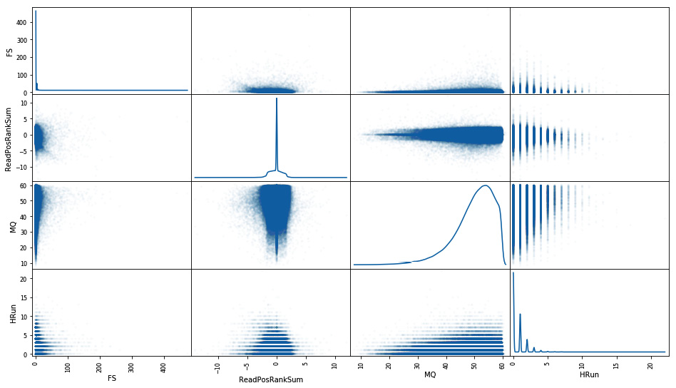
Figure 4.6 - Scatter matrix of annotations of good calls for an area of the search space

10. Finally, let’s see how our rules would perform on the complete dataset (remember that we are using a dataset roughly composed of 50% errors and 50% OK calls):

    all_fit_df = pd.DataFrame(np.load(gzip.open('feature_fit.npy.gz', 'rb')), columns=ordered_features + ['pos', 'error'])

    potentially_good_corner_df = all_fit_df[(all_fit_df['QUAL']<0.005)&(all_fit_df['QD']<0.05)]

    all_errors_df=all_fit_df[all_fit_df['error'] == 1]

    print(len(all_fit_df), len(all_errors_df), len(all_errors_df) / len(all_fit_df))

We get the following:

10905732 541688 0.04967002673456491

Let’s remember that there are roughly 10.9 million markers in our full dataset, with around 5% errors.

11. Let’s get some statistics on our good_corner:

    potentially_good_corner_errors_df = potentially_good_corner_df[potentially_good_corner_df['error'] == 1]

    print(len(potentially_good_corner_df), len(potentially_good_corner_errors_df), len(potentially_good_corner_errors_df) / len(potentially_good_corner_df))

    print(len(potentially_good_corner_df)/len(all_fit_df))

The output is as follows:

9625754 32180 0.0033431147315836243

0.8826325458942141

So, we reduced the error rate to 0.33% (from 5%), while having only reduced to 9.6 million markers.

There’s more…

Is a reduction in error from 5% to 0.3% while losing 12% of markers good or bad? Well, it depends on what analysis you want to do next. Maybe your method is resilient to loss of markers but not too many errors, in which case this might help. But if it is the other way around, maybe you prefer to have the complete dataset even if it has more errors. If you apply different methods, maybe you will use different datasets from method to method. In the specific case of this Anopheles dataset, there is so much data that reducing the size will probably be fine for almost anything. But if you have fewer markers, you will have to assess your needs in terms of markers and quality.

Finding genomic features from sequencing annotations

We will conclude this chapter and this book with a simple recipe that suggests that sometimes you can learn important things from simple unexpected results, and that apparent quality issues might mask important biological questions.

We will plot read depth – DP – across chromosome arm 2L for all the parents on our crosses. The recipe can be found in Chapter04/2L.py.

How to do it…

We’ll get started with the following steps:

1. Let’s start with the usual imports:

   from collections import defaultdict

   import gzip

   import numpy as np

   import matplotlib.pylab as plt

2. Let’s load the data that we saved in the first recipe:

   num_parents = 8

   dp_2L = np.load(gzip.open('DP_2L.npy.gz', 'rb'))

   print(dp_2L.shape)

3. And let’s print the median DP for the whole chromosome arm, and a part of it in the middle for all parents:

   for i in range(num_parents):

       print(np.median(dp_2L[:,i]), np.median(dp_2L[50000:150000,i]))

The output is as follows:

17.0 14.0

23.0 22.0

31.0 29.0

28.0 24.0

32.0 27.0

31.0 31.0

25.0 24.0

24.0 20.0

Interestingly, the median for the whole chromosome sometimes does not hold for that big region in the middle, so let’s dig further.

4. We will print the median DP for 200,000 kbp windows across the chromosome arm. Let’s start with the window code:

   window_size = 200000

   parent_DP_windows = [defaultdict(list) for i in range(num_parents)]

   def insert_in_window(row):

       for parent in range(num_parents):

           parent_DP_windows[parent][row[-1] // window_size].append(row[parent])

   insert_in_window_v = np.vectorize(insert_in_window, signature='(n)->()')

   _ = insert_in_window_v(dp_2L)

5. Let’s plot it:

   fig, axs = plt.subplots(2, num_parents // 2, figsize=(16, 9), sharex=True, sharey=True, squeeze=True)

   for parent in range(num_parents):

       ax = axs[parent // 4][parent % 4]

       parent_data = parent_DP_windows[parent]

       ax.set_ylim(10, 40)

       ax.plot(*zip(*[(win*window_size, np.mean(lst)) for win, lst in parent_data.items()]), '.')

6. The following plot shows the output:

Figure 4.7 - Median DP per window for all parents of the dataset on chromosome arm 2L

You will notice that for some mosquitoes, for example, the ones on the first and last columns, there is a clear drop of DP in the middle of the chromosome arm. In some of them, such as in the third column, there is a bit of drop – not so pronounced. And for the bottom parent of the second column, there is no drop at all.

There’s more…

The preceding pattern has a biological cause that ends up having consequences for sequencing: Anopheles mosquitoes might have a big chromosomal inversion in the middle of arm 2L. Karyotypes that are not the same as those on the reference genome used to make the calls are harder to call due to evolutionary divergence. These make the number of sequencer reads in that area lower. This is very specific to this species, but you might expect other kinds of features to appear in other organisms.

A more widely known case is Copy Number Variation (CNV): if a reference genome has only a copy of a feature, but the individual that you are sequencing has n, then you can expect to see a DP of n times the median across the genome.

But, in the general case, it is a good idea to be on the lookout for strange results throughout the analysis. Sometimes, that is the hallmark of an interesting biological feature, as it is here. Either that, or it’s a pointer to a mistake: for example, Principal Components Analysis (PCA) can be used to find mislabeled samples (as they might cluster in the wrong group).

Doing metagenomics with QIIME 2 Python API

Wikipedia says that metagenomics is the study of genetic material that’s recovered directly from environmental samples. Note that “environment” here should be interpreted broadly: in the case of our example, we will deal with gastrointestinal microbiomes in a study of a fecal microbiome transplant in children with gastrointestinal problems. The study is one of the tutorials of QIIME 2, which is one of the most widely used applications for data analysis in metagenomics. QIIME 2 has several interfaces: a GUI, a command line, and a Python API called the Artifact API.

Tomasz Kościółek has an outstanding tutorial for using the Artifact API based on the most well-developed (client-based, not artifact-based) tutorial on QIIME 2, the “Moving Pictures” tutorial (http://nbviewer.jupyter.org/gist/tkosciol/29de5198a4be81559a075756c2490fde). Here, we will create a Python version of the fecal microbiota transplant study that’s available, as with the client interface, at https://docs.qiime2.org/2022.2/tutorials/fmt/. You should get familiar with it as we won’t go into the details of the biology here. I do follow a more convoluted route than Tomasz: this will allow you to get a bit more acquainted with QIIME 2 Python internals. After you get this experience, you will probably want to follow Tomasz’s route, not mine. However, the experience you get here will make you more comfortable and confident with QIIME’s internals.

Getting ready

This recipe is slightly more complicated to set up. We will have to create a conda environment where packages from QIIME 2 are segregated from packages from all other applications. The steps that you need to follow are simple.

On OS X, use the following code to create a new conda environment:

wget wget https://data.qiime2.org/distro/core/qiime2-2022.2-py38-osx-conda.yml

conda env create -n qiime2-2022.2 --file qiime2-2022.2-py38-osx-conda.yml

On Linux, use the following code to create the environment:

wget wget https://data.qiime2.org/distro/core/qiime2-2022.2-py38-linux-conda.yml

conda env create -n qiime2-2022.2 --file qiime2-2022.2-py38-linux-conda.yml

If these instructions do not work, check the QIIME 2 website for an updated version (https://docs.qiime2.org/2022.2/install/native). QIIME 2 is updated regularly.

At this stage, you need to enter the QIIME 2 conda environment by using source activate qiime2-2022.2. If you want to get to the standard conda environment, use source deactivate instead. We will want to install jupyter lab and jupytext:

conda install jupyterlab jupytext

You might want to install other packages you want inside QIIME 2’s environment using conda install.

To prepare for Jupyter execution, you should install the QIIME 2 extension, as follows:

jupyter serverextension enable --py qiime2 --sys-prefix

TIP

The extension is highly interactive and allows you to look at data from different viewpoints that cannot be captured in this book. The downside is that it won’t work in nbviewer (some cell outputs won’t be visible with the static viewer). Remember to interact with the outputs from the extension, since many are dynamic.

You can now start Jupyter. The notebook can be found in the Chapter4/QIIME2_Metagenomics.py file.

WARNING

Due to the fluidity of package installation with QIIME, we don’t provide a Docker environment for it. This means that if you are working from our Docker installation you will have to download the recipe and install the packages manually.

You can find the instructions to get the data of both the Notebook files and the QIIME 2 tutorial.

How to do it...

Let’s take a look at the following steps:

1. Let’s start by checking what plugins are available:

   import pandas as pd

   from qiime2.metadata.metadata import Metadata

   from qiime2.metadata.metadata import CategoricalMetadataColumn

   from qiime2.sdk import Artifact

   from qiime2.sdk import PluginManager

   from qiime2.sdk import Result

   pm = PluginManager()

   demux_plugin = pm.plugins['demux']

   #demux_emp_single = demux_plugin.actions['emp_single']

   demux_summarize = demux_plugin.actions['summarize']

   print(pm.plugins)

We are also accessing the demultiplexing plugin and its summarize action.

2. Let’s take a peek at the summarize action, namely inputs, outputs, and parameters:

   print(demux_summarize.description)

   demux_summarize_signature = demux_summarize.signature

   print(demux_summarize_signature.inputs)

   print(demux_summarize_signature.parameters)

   print(demux_summarize_signature.outputs)

The output will be as follows:

Summarize counts per sample for all samples, and generate interactive positional quality plots based on `n` randomly selected sequences.

OrderedDict([('data', ParameterSpec(qiime_type=SampleData[JoinedSequencesWithQuality | PairedEndSequencesWithQuality | SequencesWithQuality], view_type=<class 'q2_demux._summarize._visualizer._PlotQualView'>, default=NOVALUE, description='The demultiplexed sequences to be summarized.'))])

OrderedDict([('n', ParameterSpec(qiime_type=Int, view_type=<class 'int'>, default=10000, description='The number of sequences that should be selected at random for quality score plots. The quality plots will present the average positional qualities across all of the sequences selected. If input sequences are paired end, plots will be generated for both forward and reverse reads for the same `n` sequences.'))])

OrderedDict([('visualization', ParameterSpec(qiime_type=Visualization, view_type=None, default=NOVALUE, description=NOVALUE))])

3. We will now load the first dataset, demultiplex it, and visualize some demultiplexing statistics:

   seqs1 = Result.load('fmt-tutorial-demux-1-10p.qza')

   sum_data1 = demux_summarize(seqs1)

   sum_data1.visualization

Here is a part of the output from the QIIME extension for Juypter:

Figure 4.8 - A part of the output of the QIIME2 extension for Jupyter

Remember that the extension is iterative and provides substantially more information than only this chart.

TIP

The original data for this recipe is supplied in QIIME 2 format. Obviously, you will have your own original data in some other format (probably FASTQ) – see the There’s more... section for a way to load a standard format.

QIIME 2’s .qza and .qzv formats are simply zipped files. You can have a look at the content with unzip.

The chart will be similar to in the QIIME CLI tutorial, but be sure to check the interactive quality plot of our output.

4. Let’s do the same for the second dataset:

   seqs2 = Result.load('fmt-tutorial-demux-2-10p.qza')

   sum_data2 = demux_summarize(seqs2)

   sum_data2.visualization

5. Let’s use the DADA2 (https://github.com/benjjneb/dada2) plugin for quality control:

   dada2_plugin = pm.plugins['dada2']

   dada2_denoise_single = dada2_plugin.actions['denoise_single']

   qual_control1 = dada2_denoise_single(demultiplexed_seqs=seqs1,

                                       trunc_len=150, trim_left=13)

   qual_control2 = dada2_denoise_single(demultiplexed_seqs=seqs2,

                                       trunc_len=150, trim_left=13)

6. Let’s extract some statistics from denoising (first set):

   metadata_plugin = pm.plugins['metadata']

   metadata_tabulate = metadata_plugin.actions['tabulate']

   stats_meta1 = metadata_tabulate(input=qual_control1.denoising_stats.view(Metadata))

   stats_meta1.visualization

Again, the result can be found online in the QIIME 2 CLI version of the tutorial.

7. Now, let’s do the same for the second set:

   stats_meta2 = metadata_tabulate(input=qual_control2.denoising_stats.view(Metadata))

   stats_meta2.visualization

8. Now, merge the denoised data:

   ft_plugin = pm.plugins['feature-table']

   ft_merge = ft_plugin.actions['merge']

   ft_merge_seqs = ft_plugin.actions['merge_seqs']

   ft_summarize = ft_plugin.actions['summarize']

   ft_tab_seqs = ft_plugin.actions['tabulate_seqs']

   table_merge = ft_merge(tables=[qual_control1.table, qual_control2.table])

   seqs_merge = ft_merge_seqs(data=[qual_control1.representative_sequences, qual_control2.representative_sequences])

9. Then, gather some quality statistics from the merge:

   ft_sum = ft_summarize(table=table_merge.merged_table)

   ft_sum.visualization

10. Finally, let’s get some information about the merged sequences:

    tab_seqs = ft_tab_seqs(data=seqs_merge.merged_data)

    tab_seqs.visualization

There’s more...

The preceding code does not show you how to import data. The actual code will vary from case to case (single-end data, paired-end data, or already-demultiplexed data), but for the main QIIME 2 tutorial, Moving Pictures, assuming that you have downloaded the single-end, non-demultiplexed data and barcodes into a directory called data, you can do the following:

data_type = 'EMPSingleEndSequences'
conv = Artifact.import_data(data_type, 'data')
conv.save('out.qza')

As stated in the preceding code, if you look on GitHub for this notebook, the static nbviewer system will not be able to render the notebook correctly (you have to run it yourself). This is far from perfect; it is not interactive, since the quality is not great, but at least it lets you get an idea of the output without running the code.