
9
Machine Learning for Sensor Networks
9.1 Introduction
‘Machine learning’ refers to a combination of learning from data and their clustering or classification. It is often combined with some signal processing techniques to extract the best discriminating features of the data prior to taking learning and classification steps. The emerging machine learning techniques, such as deep neural networks (DNNs), are also capable of feature learning.
Often, in body sensor networks (BSNs), multimodal data are used, and thus features from various measurement modalities should be combined or exploited. This leads to another area in machine learning called sensor (data) fusion.
Sensors are used almost everywhere. The newly emerging sensor technology is beginning to closely mimic the ultimate sensing machine, i.e. the human being. The sensor fusion technology leverages a microcontroller (which mimics the human brain) to fuse individual data collected by multiple sensors. This allows for a more accurate and reliable realisation of the data than one would acquire from an individual sensor.
Sensor fusion enables context awareness, which has significant potential for the Internet of Things (IoT). Advances in sensor fusion for remote emotive computing (emotion sensing and processing) could also lead to exciting new applications in the future, including smart healthcare. This approach motivates personalised healthcare providers to fine tune and customise systems which best suit individuals' needs.
However, new technology is shifting towards consensus or diffusion communication networks whereby sensors can communicate to each other and decide on their next action without communicating to any hub or master node. Unlike current systems, this is a decentralised approach in which the decision is made at each sensor. This also brings a new direction in machine learning called cooperative learning, which exploits the information from a number of sensors in a neighbourhood to decide on the action of each sensor within that neighbourhood.
There are mainly two types of machine learning algorithms for classification of data: supervised and unsupervised. In an unsupervised learning algorithm the classifier clusters the data into the groups farthest from each other. A popular example for these algorithms is k-means algorithm. On the other hand, for supervised classifiers, the target is known during the training phase and the classifier is trained to minimise a difference between the actual output and the target values. Traditional methods based on adaptive filters using mean squared error (MSE) or least square error (LSE) minimisations are still in use. Good examples of such classifiers are support vector machines (SVM), and multilayered perceptron (MLP). In both cases, effective estimation of data features often helps reduce the number of input samples, thus enhancing the overall algorithm speed. The more efficiently the features are estimated, the more accurate the result of the clustering or classification will be.
Many algorithms can be used for feature estimation. These algorithms are often capable of changing the dimensionality of the signals to make them more separable. Numerous statistical measures can be derived from the data with known distributions. Various order statistics such as mean, variance, skewness, and kurtosis are very popular statistical measures to describe the data in scalar forms. The vector forms may become necessary for multichannel data.
In addition to the above two main classes of learning systems, semi-supervised techniques benefit from partially known information during training or classification. This group of learning systems benefits from various constraints on the input, output, or classifier in order to best optimise the system for each particular application. One useful application of such systems is for the rejection of anomalies in the datasets during classifier training [1].
In the clustering methods there is no need to label the classes in advance and only the number of clusters may be identified and fed into the clustering algorithm by the user. Classification of data is similar to clustering, except the classifier is trained using a set of labelled data before being able to classify a new data. In practice, the objective of classification is to draw a boundary between two or more classes and to label them based on their measured features. In a multidimensional feature space this boundary takes the form of a separating hyperplane. The objective here is to find the best hyperplane, maximising the distance from all the classes (interclass members) while minimising proximities within members of each class (intraclass members).
Clustering and classification become ambiguous when deciding which features to use and how to extract or enhance those features. Principal component analysis (PCA) and independent component analysis (ICA) are two very common approaches to extract the dominant data features. Traditionally, a wide range of features (such as various order statistics) are measured or estimated from the raw data and used by the machine learning algorithms for clustering or classification.
In the context of human-related signals, classification of the data in feature space is often required. For example, the power of alpha and beta waves in electroencephalography (EEG) signals [2] may be classified to not only detect the brain abnormalities but also determine the stage of the disease. In sleep studies, one can look at the power of alpha and theta waves as well as appearance of spindles and K-complexes to classify the stages of sleep. As another example, in brain–computer interfacing (BCI) systems for left and right finger movement detection one needs to classify the time, frequency, and spatial features.
There have been several popular machine learning approaches developed in the past 50 years. Among them artificial neural networks (ANNs), linear discriminant analysis (LDA), hidden Markov model (HMM), Gaussian mixture model (GMM), decision tree, random forest, and SVMs are the most popular ones. k-mean clustering and fuzzy logic have also been widely used for clustering, pre-classification, and other artificial intelligent (AI) based applications [3]. These techniques are developed and well explained in the literature [4]. Detailed explanation of all these methods is beyond the objective of this chapter. Instead, here we provide a summary of the most popular machine learning methods which have been widely used in sensor networking and health-related data analysis.
Unlike many mathematical problems in which some forms of explicit formula based on a number of inputs results in an output, in data classification there is no model or formula of this kind. Instead, the system should be trained (using labelled data) to be able to recognise the new (test) inputs.
In the case of data with considerable noise or artefacts, successful classifiers are those which can minimise the effect of outliers. Outliers are the data samples or features which turn up very distant from the class centres, and therefore they do not belong to any class. In many machine learning algorithms, outliers have destructive effect during the classifier training and increase the cross-validation error. Pre-processing (including smoothing, denoising, etc.) can significantly reduce the outliers or their impact. Right choice of classifiers and their associated feature detection systems can also reduce the influence of outliers.
For sensor network applications, machine learning is important since:
- Sensor networks usually monitor dynamic environments which rapidly change over time. It is therefore desirable to develop sensor networks that can adapt and operate efficiently in such environments.
- Sensor networks may be used to collect new information about unreachable and risky locations such as inside the body [5]. Owing to the unexpected behaviour patterns that may arise in such scenarios, the initial solutions provided by system designers may not operate as expected. Thus, robust machine learning algorithms, able to calibrate itself to newly acquired information, would be desirable.
- The sensors may be deployed in complicated environments where the researchers cannot build accurate mathematical models to describe the system behaviour. Meanwhile, some tasks in wireless sensor networks (WSNs) can be prescribed using simple mathematical models but may still need complex algorithms to solve them (e.g. the routing problem [6, 7]). In such circumstances, machine learning circumvents the problem and provides low-complexity estimates for the system model.
- Sensor networks often provide large amounts of data but may not be able to make clear sense of them. For example, in addition to ensuring communication connectivity and energy sustainability, WSN application often comes with minimum data coverage requirements which need to be fulfilled by limited sensor hardware resources [8]. Machine learning techniques can then be used to discover the data and recognise important correlations in the sensor data before proposing an improved sensor deployment for maximum data coverage.
- New applications and integrations of WSNs – such as in-patient status monitoring, cyber-physical systems (CPSs), machine-to-machine (M2M) communications, and IoT technologies – have been introduced with a motivation to support more intelligent decision making and autonomous control [9]. Here, machine learning is important to extract the different levels of abstractions necessary to perform the AI tasks with limited human intervention [10].
Many machine learning algorithms do not perform efficiently when
- The number of features or input samples is high.
- There is a limited time to perform the classification.
- There is a nonuniform weighting amongst features.
- There is a nonlinear map between inputs and outputs.
- Distribution of data is not known.
- There are significant number of outliers.
- The convergence of the algorithm is not convex (monotonic), so it may fall into a local minimum.
In addition, in using machine learning for sensor networks:
- Being a resource limited framework, WSN with a distributed management system drains a considerable percentage of its energy budget for conditioning, pre-processing, or processing the data samples. Thus, a trade-off between the algorithm's computational requirements and the learnt model's accuracy has to be taken into consideration. Specifically, the higher the required accuracy, the higher the computational requirements and the higher energy consumptions are.
- Generally speaking, learning by synthetic or simulated data requires a large dataset of samples to achieve the intended generalisation capabilities (i.e. fairly small error bounds), and there won't be a full control over the knowledge formulation process [11].
For the data with unknown distributions often nonparametric techniques are applied. In these techniques a subset of labelled data is used to estimate or model the data distributions through learning before application of any feature selection or classification algorithm.
To assess the performance quality of the classifiers a multifold cross-validation is often necessary. For this, only the training data are considered. In each fold a percentage of the labelled data is used to train the classifier and the rest used for testing. The cross-validation error is then calculated as the amount of misclassified data over a number of folds, say k-fold.
Lastly, but probably most importantly, is dimensionality reduction. Dimensionality reduction plays an important role in machine learning mainly for high-dimensionality datasets, where the number of available features is large. Reducing dimensionality often alleviates the effect of outliers and noise and therefore enhances the classifier performance. PCA is the most popular dimensionality reduction technique. PCA projects the data into a lower dimensional space using singular value decomposition (SVD), X = UΣVT where U and V are singular vectors and Σ represents the square matrix of singular values or eigenvalues. Input to SVD can have mixed-signs. Nonnegative matrix factorisation (NMF), as another approach, restricts factors to be nonnegative and can be used when the input data is nonnegative. Hence, it works based on setting a nonnegativity constraint on the extracted components, X+ = W+H+ where (.)+ represents the nonnegativity of all elements of the input data and components. Binary matrix factorisation is another extension of NMF for the binary data by constraining components to be binary, X0–1 = W0–1H0–1 where (.)0–1 represents the binary elements. Sparsity constraints (by constraining factorised components' norm) can be added to the optimisation of PCA and NMF to enhance the interoperability and stability of components: SPCA (sparse principal component analysis) and SNMF (sparse non-negative matrix factorisation). Sparsity constraints are particularly important where the data are naturally sparse [12].
9.2 Clustering Approaches
9.2.1 k-means Clustering Algorithm
k-means algorithm [13] is an effective and, generally, simple clustering tool that has been widely used for many applications, such as discovering spike patterns in neural responses [14]. It is employed either for clustering only or as a method to find the target values (cluster centres) for a supervised classification in a later stage. This algorithm divides a set of features (such as points in Figure 9.1) into k-clusters.
The algorithm is initialised by setting ‘C’ as the desired or expected number of clusters. Then, the centre for each cluster k is identified by selecting k representative data points. The next step is to assign the remaining data points to the closest cluster centre. Mathematically, this means that each data point needs to be compared with every existing cluster centre and the minimum distance between the point and the cluster centre found. Most often, this is performed in the form of error checking (which is discussed below). However, prior to this, the new cluster centres are calculated. This is essentially the remaining step in k-means clustering: once clusters have been established (i.e. each data point is assigned to its closest cluster centre), the geometric centre of each cluster is recalculated.
The Euclidean distance of each data point within a cluster to its centre can be calculated. This can be repeated for all other clusters, whose resulting sums can themselves be summed together. The final sum is known as the sum of within-cluster sum-of-squares. Consider the within-cluster variation (sum of squares for cluster c) error as εc:
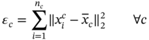
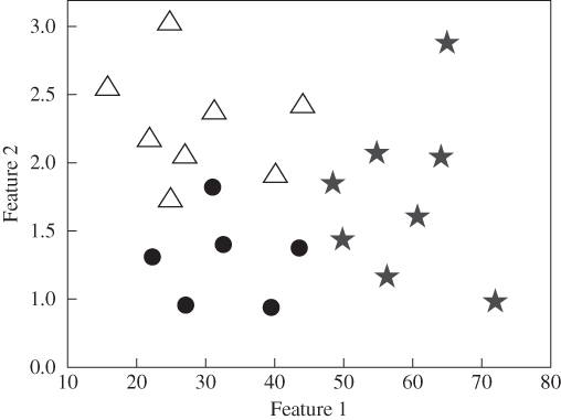
Figure 9.1 A 2D feature space with three clusters, each with members of different shapes (circle, triangle, and asterisk).
where ![]() is the squared Euclidean distance between data point i and its designated cluster centre
is the squared Euclidean distance between data point i and its designated cluster centre ![]() , nc is the total number of data points (features) in cluster c, and
, nc is the total number of data points (features) in cluster c, and ![]() is an individual data point in cluster c. The cluster centre (mean of data points in cluster c) can be defined as:
is an individual data point in cluster c. The cluster centre (mean of data points in cluster c) can be defined as:
and the total error is:

The overall k-means algorithm may be summarised as:
- Initialisation
- Define the number of clusters (C).
- Designate a cluster centre (a vector quantity that is of the same dimensionality of the data) for each cluster, typically chosen from the available data points.
- Assign each remaining data point to the closest cluster centre. That data point is now a member of that cluster.
- Calculate the new cluster centre (the geometric average of all the members of a certain cluster).
- Calculate the sum of within-cluster sum-of-squares. If this value has not significantly changed over a certain number of iterations, stop the iterations. Otherwise, go back to Step1.
Therefore, an optimum clustering procedure depends on an accurate estimation of the number of clusters. A common problem in k-means partitioning is that if the initial partitions are not chosen carefully enough the computation will run the chance of converging to a local minimum rather than the global minimum solution. The initialisation step is therefore very important.
9.2.2 Iterative Self-organising Data Analysis Technique
One way to estimate the number of clusters is to run the algorithm several times with different initialisations and by iteratively increasing the number of clusters from the lowest value. If the results converge to the same partitions, then it is likely that a global minimum has been reached. However, this is very time consuming and computationally expensive. Another solution is to dynamically change the number of partitions (i.e. number of clusters) as the iterations progress. The ISODATA (iterative self-organising data analysis technique algorithm) is an improvement on the original k-means algorithm that does exactly this. ISODATA involves a number of additional parameters into the algorithm allowing it to progressively check within- and between-cluster similarities so that the clusters can dynamically split and merge.
9.2.3 Gap Statistics
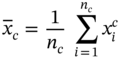
Another approach for solving this problem is gap statistics [15]. In this approach the number of clusters is iteratively estimated. The steps of this algorithm are:
- For a varying number of clusters k = 1, 2, …, C, compute the error Ec using Eq. (9.3).
- Generate a B number of reference datasets. Cluster each one with the k-means algorithm and compute the dispersion measures,
 , b = 1, 2, …, B. The gap statistics are then estimated using:
(9.4)
, b = 1, 2, …, B. The gap statistics are then estimated using:
(9.4)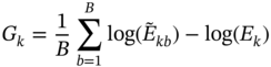
where the dispersion measure
 is the Ek of the reference dataset B.
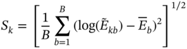
 - To account for the sample error in approximating an ensemble average with B reference distributions, compute the standard deviation Sk as:
(9.5)
where:
(9.6)
- By defining
 , estimate the number of clusters as the smallest k such that
 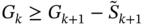 ,
, - With the number of clusters identified, utilise k-means algorithm to partition the feature space into k subsets (clusters).
The above clustering method has several advantages over k-means since it can estimate the number of clusters within the feature space. It is also a multiclass clustering system and unlike SVM can provide the boundary between the clusters.
9.2.4 Density-based Clustering
The density-based clustering approach clusters the point features within surrounding noise based on their spatial distribution. It works by detecting areas where the points are concentrated and are separated by areas that are empty or sparse. Points that are not part of a cluster are labelled as noise. In this clustering method unsupervised machine learning clustering algorithms are used, which automatically detect patterns based purely on spatial location and the distance to a specified number of neighbours. These algorithms are considered unsupervised as they do not need any training on what it means to be a cluster [16].
Density-based spatial clustering of applications with noise (DBSCAN) is a popular density-based clustering algorithm with the aim of discovering clusters from approximate density distribution of the corresponding data points. DBSCAN does not need the number of clusters, and instead has two parameters to be set: an epsilon that indicates the closeness of the points in each and minPts, the minimum neighbourhood size a point should fall into to be considered a member of that cluster. The routine is initialised randomly. The neighbourhood of this point then retrieved and if it consists of an acceptable number of elements, a cluster is formed; otherwise, the element is considered as noise. Hence, DBSCAN may result in some samples which are not clustered.
Usually, DBSCAN parameters are not known in advance and there are several ways to select their values. One way is to calculate the distance of each point to its closest nearest neighbour and use the histogram of distances to select epsilon. Then, a histogram can be obtained of the average number of neighbours for each point using the epsilon. Some of the samples do not have enough any neighbouring point and are counted as noise samples. Implementation of the parameter selection is available at spark DBSCAN (https://github.com/alitouka/spark_dbscan).
DBSCAN can find arbitrary-shaped clusters and is robust to outliers. Nevertheless, it may not identify clusters of various densities or may fail if the data are very sparse. It is also sensitive to the selection of its parameters and the distance measure (usually Euclidean distance), which affects other clustering techniques too.
9.2.5 Affinity-based Clustering
This combines k-means clustering with a spectral-based clustering method where the algorithms cluster the points using eigenvectors of matrices derived from the data. It uses k eigenvectors simultaneously and identifies the best setting under which the algorithm can perform favourably [17].
9.2.6 Deep Clustering
Deep clustering is another modification to clustering which combines k-means with neural network (NN) to jointly learn the parameters of an NN and the cluster assignments of the resulting features. It iteratively groups the features using a k-means and uses the subsequent assignments as supervision to update the weights of the network. This organises an unsupervised training of convolutional neural networks (CNNs). This approach, demonstrated in Figure 9.2, is similar to the standard supervised training of a CNN and it integrates CNN in its structure [18]. The CNN is explained later in this chapter.
In addition to the above clustering approaches, there are other clustering methods such as power iteration clustering (PIC) [19], which use similar concepts. PIC finds a very low-dimensional embedding of a dataset using truncated power iteration on a normalised pair-wise similarity matrix of the data. It has been shown that it is fast for processing large datasets.
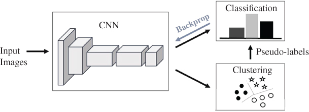
Figure 9.2 Schematic diagram of deep clustering [17]. The deep features are iteratively clustered and the cluster assignments are used as pseudo-labels to learn the parameters of a CNN.
Source: Courtesy of Ng, Y.A., Jordan, M.I., and Weiss, Y.
9.2.7 Semi-supervised Clustering
Conventional clustering methods are unsupervised, meaning that there is no available label (target) or anything known about the relationship between the observations in the dataset. In many situations, however, information about the clusters is available in addition to the feature values. For example, the cluster labels of some observations may be known, or certain observations may be known to belong to the same cluster. In other cases, one may wish to identify clusters that are associated with a particular outcome (or target).
The main purposes for so-called semi-supervised methods are the accurate determination of number of clusters and the minimisation of clustering error. Very similar to the concept in Section 9.2.6, there are semi-supervised clustering techniques where supervised and unsupervised learnings are combined to iteratively improve the performance of clustering methods in terms of number of clusters and clustering error. Among these algorithms, deep networks are often used for supervised clustering [17, 20, 21]. The algorithm in [20] simultaneously minimises the sum of supervised and unsupervised cost functions by backpropagation.
9.2.7.1 Basic Semi-supervised Techniques
Two basic semi-supervised techniques are label spreading (LS) and label propagation (LP). LS is based on considering samples (isolates) as nodes in a graph in which their relations defined by edge weights, for example wij = exp(−∥xi − xj∥2/2σ2) if i ≠ j and wij = 0. The weight matrix is symmetrically normalised for better convergence. Each node receives information from its neighbouring points and its label is selected based on the class with most received information. A regularisation term was also introduced for a better label assignment based on having a smooth classifier (not changing between similar points). LP is based on an iterative technique considering a transition matrix to update labels which starts with a random initialisation. The transition matrix refers to the probability of moving from one node to another by propagating in high-density areas of the unlabelled data.
9.2.7.2 Deep Semi-supervised Techniques
As described in a later section of this chapter, autoencoder (AE) is a DNN which has two main stages: an encoder that maps the input space to a lower dimension (latent space) and a decoder that reconstructs the input space back from the latent representation. Hence, the network is based on an unsupervised learning. AE can be stacked to form a deep stacked autoencoder (SAE) network that adds more power to the network and provides nonlinear latent representations per each hidden layer. Moreover, to improve generalisation and increasing possibility of extracting more interesting patterns in the data, various noise levels can be added to the input of each layer, denoted as stacked denoising autoencoder (SDAE). The optimisation for SDAE is based on minimising the reconstruction error between the original data and the predicted network output.
Although AE, SAE, and SDAE are based on unsupervised learning (using the reconstruction error), they have been used for semi-supervised learning by adding a layer to the learnt encoders and fine tuning the network based on the labelled data for the supervised task (supervised SDAE). The main disadvantage of this technique is to have two stages for supervised and unsupervised learning. Consequently, the first stage may extract information that are not useful for the final supervised task. Owing to this, the fine-tuning stage cannot extensively change a fully learnt network.
Ladder is an extension of SAE/SDAE considering a joint objective function of reconstruction error for unsupervised learning and likelihood of estimating the correct labels for supervised learning. It has two noiseless and noisy encoder paths and a denoising decoder.
9.2.8 Fuzzy Clustering
In this clustering method each element has a set of membership coefficients corresponding to the degree of being in a given cluster [22]. This is different from k-means, where each object belongs exactly to one cluster. For this reason, unlike k-means, which is known as hard or nonfuzzy clustering, this is called the soft clustering method.
In fuzzy clustering, points close to the centre of a cluster may be in the cluster to a higher degree than points in the edge of a cluster. The degree to which an element belongs to a given cluster is a numerical value varying from 0 to 1.
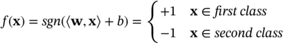
However, fuzzy c-means (FCM), the most widely used fuzzy clustering algorithms, is very similar to k-means. In FCM the centroid of a cluster is calculated as the mean of all points, weighted by their degree of belonging to the cluster. The aim of c-means is to cluster the points into k cluster by minimising the objective function defined as:
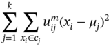
where μj is the centre of the cluster j, m the fuzzifier, often selected manually, and ![]() is the degree to which an observation xi belongs to a cluster cj, defined as:
is the degree to which an observation xi belongs to a cluster cj, defined as:
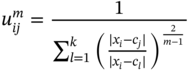
The degree of belonging, ![]() , is linked inversely to the distance from x to the cluster centre.
, is linked inversely to the distance from x to the cluster centre.
The parameter m is a real number within 1.0 < m < ∞ and defines the level of cluster fuzziness. For m close to 1 the solution becomes very similar to hard clustering such as k-means, whereas a value of m close to infinity leads to complete fuzzyness. The centroid of a cluster, cj, is the mean of all points, weighted by their degree of belonging to the cluster:
The algorithm of fuzzy clustering can be summarised as follow:
- Set the number of clusters k.
- Assign randomly to each point coefficients for being in the clusters.
- Repeat until the maximum number of iterations is reached, or when the algorithm has converged for a predefined error:
This concludes the well-established clustering approaches. Other clustering methods such as k-medoid are very similar to the above methods. Most of these methods are sensitive to outliers and the objective of new weighted or regularised techniques is to reduce this sensitivity.
9.3 Classification Algorithms
9.3.1 Decision Trees
Decision trees (DTs) are popular, simple, powerful, and generally nonlinear tools for classification and prediction. They represent rules which can be deciphered by human beings and utilised in knowledge-based systems.
The main steps in a DT algorithm are:
- Select the best attribute(s) to split the remaining instances and make that attribute a decision node.
- Repeating this process recursively for each child.
- Stop when:
- All the instances have the same target attribute value.
- There are no more attributes.
- There are no more instances.
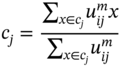
One simple DT example for a humidity sensor can be:
If the time is 9:00 a.m. and there is no rain what would be the humidity level (out of low, medium, and severe)?
Depending on the number of attributes, a DT may look like Figure 9.3. DTs can perfectly be fitted to any training data, with zero bias and high variance. Different algorithms are used to determine the ‘best’ split at a node.
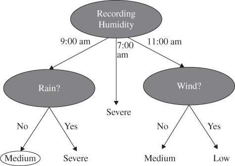
Figure 9.3 An example of a DT to show the humidity level at 9 a.m. when there is no rain.
DTs are often used to predict data labels by iterating the input data through a learning tree [23]. During this process, the feature properties are compared relative to the decision conditions to reach a specific category. Among many applications, a DT provides a simple, but efficient method to identify link reliability in WSNs by identifying a few critical features such as loss rate, corruption rate, mean time to failure (MTTF) and mean time to restore (MTTR). However, DT works only with linearly separable data and the process of building optimal learning trees is NP (neural process) complete [24]. DT-based sensor activity recognition and detection is one practical example [25].
9.3.2 Random Forest
A random forest (or random forests) classifier creates a set of DTs from randomly selected subsets of training set. It then aggregates the votes from different DTs to decide the final class of the test data [26]. The term random forest comes from random decision forests initially proposed by Tin Kam Ho of Bell Labs in 1995. This method combines Breiman's ‘bagging’ idea and random feature selection. Bagging or bootstrap aggregation is a technique for reducing the variance of an estimated prediction function. Random forest classifier is in fact an extension to bagging which uses de-correlated trees.
The main advantages of random forest classifiers are that there is no need for pruning trees, accuracy, and variable importance are generated automatically, overfitting is not a problem, they are not very sensitive to outliers in training data, and setting their parameters is easy.
However, there are some limitations: the regression process cannot predict beyond the available range in the training data and in regression the extreme values are often not predicted accurately. This causes underestimation of highs and overestimation of lows.
Unlike for a traditional random forest, which is a bagging technique, in boosting as the name suggests, one learns from other which in turn boosts the learning. The bagging scheme trains a bunch of individual models in a parallel way. Each model is trained by a random subset of the data. On the other hand, boosting trains a bunch of individual models in a sequential way. Each individual model learns from the mistakes made by the previous model. AdaBoost is a boosting ensemble model and performs well with the DT. AdaBoost learns from the mistakes by increasing the weight of misclassified data points. The optimisation of AdaBoost is sometimes by means of adaptive methods, such as gradient decent, and therefore, AdaBoost and gradient boosting are very similar.
9.3.3 Linear Discriminant Analysis
LDA is a method used to find a linear combination of features which characterises or separates two or more classes of objects or events. The resulting combination may be used as a linear classifier. In an LDA it is assumed that the classes have normal distributions. Like PCA, an LDA is used for both dimensionality reduction and data classification.
In a two-class dataset, given the a priori probabilities for class 1 and class 2, respectively, as p1 and p2, class means and overall mean, respectively, as μ1, μ2, and μ, and the class variances as cov1 and cov2.
Then, within-class and between-class scatters are used to formulate the necessary criteria for class separability. Within-class scatter is the expected covariance of each of the classes. The scatter measures for multiclass case are computed as:

where C refers to the number of classes and:
Slightly differently, the between-class scatter is estimated as:

Then, the objective would be to find a discriminant plane, w, to maximise the ratio between between-class and within-class scatters (variances):

In practice, class means and covariances are not known but they can be estimated from the training set. In the above equations, either the maximum likelihood estimate or the maximum a posteriori estimate may be used instead of the exact values.
9.3.4 Support Vector Machines
Amongst all supervised classifiers, SVM is very popular for many applications whilst outperforming them in many linear (separable) and nonlinear (nonseparable) cases. The SVM concept was introduced by Vapnik in 1979 [27] and explored in many publications such as [28–32]. To understand the SVM concept, consider a binary classification for the simple case of a 2D feature space of linearly separable training samples S = {(x1, y1), (x2, y2), …, (xm, ym)} (Figure 9.4), where x ∈ Rd is the input vector and y ∈ {1, − 1} is the class label. A discriminating function is defined as:
In this formulation w determines the orientation of a discriminant plane (or hyperplane). Clearly, there are an infinite number of possible planes that could correctly classify the training data. An optimal classifier finds the hyperplane for which the best generalising hyperplane is equidistant or farthest from each set of points. Optimal separation is achieved when there is no separation error and the distance between the closest vector and the hyperplane is maximal.
One way to find the separating hyperplane in a separable case is by constructing the so-called convex hulls of each dataset. The encompassed regions are the convex hulls for the datasets. By examining the hulls one can then determine the closest two points lying on the hulls of each class (note that these do not necessarily coincide with actual data points). By constructing a plane perpendicular and equivalent to these two points, an optimal hyperplane with robust classifier should result.
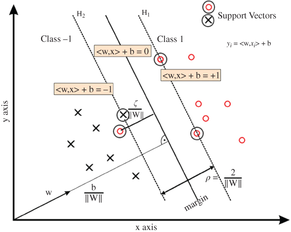
Figure 9.4 The SVM separating hyperplane and support vectors for a separable data case.
For an optimal separating hyperplane design, often few points, referred to as support vectors (SVs), are utilised (e.g. the three circled black data feature points in Figure 9.4).
SVM formulation starts with the simplest case: linear machines are trained on separable data (for general case analysis, nonlinear machines trained on nonseparable data result in a very similar quadratic programming problem). Then, the training data {xi, yi}, i = 1, …, m, yi ∈ {1, − 1}, xi ∈ Rd are labelled. Consider having a hyperplane which separates the positive from the negative examples. Points x lying on the hyperplane satisfy 〈w, x〉 + b = 0, where w is normal to the hyperplane, b/‖w‖2 is the perpendicular distance from the hyperplane to the origin, and ‖w‖2 is the Euclidean norm of w. Define the ‘margin’ of a separating hyperplane illustrated in Figure 9.4, and for the linearly separable case, the algorithm simply looks for the separating hyperplane with largest margin. Here, the approach is to reduce the problem to a convex optimisation problem by minimising a quadratic function under linear inequality constraints. To find a plane farthest from both classes of data, the margin between the supporting canonical hyperplanes for each class is maximised. The support planes are pushed apart until they meet the closest data points, which are then deemed to be the support vectors (circled in Figure 9.4). Therefore, the SVM problem to find w is stated as:
which can be combined into one set of inequalities as yi(〈xi, w〉 + b) − 1 ≥ 0 ∀ i. The margin between these supporting planes (H1 and H2) can be shown to be γ = 2/‖w‖2. Therefore, to maximise this margin we therefore need to:

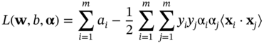
This constrained optimisation problem can be changed into an unconstrained problem by using Lagrange multipliers. This leads to minimisation of an unconstrained empirical risk function (Lagrange), which consequently results in a set of conditions called Kuhn–Tucker (KT) conditions. The new optimisation problem brings about the so-called primal form as:

where the αi, i = 1, …, m are the Lagrange multipliers. The Lagrange primal has to be minimised with respect to w, b and maximised with respect to αi ≥ 0. Constructing the classical Lagrange dual form facilitates this solution. This is achieved by setting the derivatives of the primal to zero and re-substituting them back into the primal. Hence, the dual form is derived as:
and:
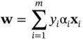
considering that ![]() and αi ≥ 0. These equations can be solved using many different publicly available quadratic programming (QP) algorithms such as those proposed at www.support-vector.net and www.kernel-machines.org.
and αi ≥ 0. These equations can be solved using many different publicly available quadratic programming (QP) algorithms such as those proposed at www.support-vector.net and www.kernel-machines.org.
In nonseparable cases where the classes have overlaps in the feature space, the maximum margin classifier described above is no longer applicable. With the help of some complicated mathematical derivations, we are often able to define a nonlinear hyperplane to accurately separate the datasets. As we will see later, this causes an overfitting problem which reduces the robustness of classifier. The ideal solution where no points are misclassified and no points lie within the margin is no longer feasible. This implies that we need to relax the constraints to allow for a minimum of misclassifications. In this case, the points that subsequently fall on the wrong side of the margin are considered errors. However, they have less influence on the location of the hyperplane (according to a pre-set slack variable) and as such are considered to be support vectors. The classifier obtained in this way is called a soft margin classifier.
To optimise the soft margin classifier, we must allow violation of the margin constraints according to a pre-set slack variable ξi in the original constraints, which then become:
and ξi ≥ 0 ∀ i
For an error to occur, the corresponding ξi must exceed unity. Therefore, ![]() is an upper bound on the number of training errors. Hence, a natural way to assign an extra cost for errors is to change the objective function to:
is an upper bound on the number of training errors. Hence, a natural way to assign an extra cost for errors is to change the objective function to:
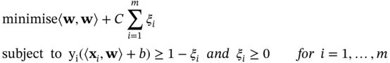
The primal form will then be:

Hence, by differentiating this cost function with respect to w, ξ, and b we can achieve:
and:
By substituting these into the primal form and again considering that ![]() and αi ≥ 0, the dual form is derived as:
and αi ≥ 0, the dual form is derived as:
This is similar to the maximal marginal classifier with the only difference in that here we have a new constraint of αi + ri = C, where ri ≥ 0, hence 0 ≤ αi ≤ C. This implies that the value C sets an upper limit on the Lagrange optimisation variables αi. This is sometimes referred to as the box constraint. The value of C offers a trade-off between accuracy of data fit and regularisation. A small value of C (i.e. C < 1) significantly limits the influence of error points (or outliers), whereas if C is chosen to be very large (or infinite) then the soft margin (as in Figure 9.5) approach becomes identical to the maximal margin classifier. Therefore, in the use of a soft margin classifier, the choice of C strongly depends on the data. Appropriate selection of C is important and itself is an area of research. One way to set C is by gradually increasing C from max (αi) for ∀i and find the value for which the error (outliers, cross validation, or number of misclassified points) is minimum. Eventually, C can be found empirically [33].
There will be no change in formulation of the SVM for multidimensional cases, only the dimension of the hyperplane changes depending on the number of feature types.
In many nonseparable cases the use of a nonlinear function may help to make the datasets separable. As can be seen in Figure 9.6, the datasets are separable if a nonlinear hyperplane is used. Kernel mapping offers an alternative solution by nonlinearly projecting the data into a (usually) higher dimensional feature space to allow the separation of such cases.
The key success to Kernel mapping is that special types of mapping that obey Mercer's theorem, sometimes called reproducing kernel Hilbert spaces (RKHSs) [27], offer an implicit mapping into feature space:
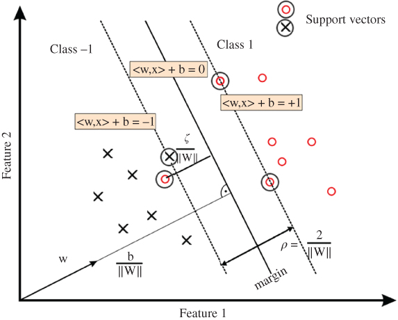
Figure 9.5 Soft margin and the concept of slack parameter.
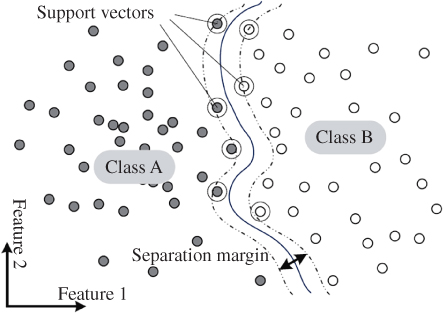
Figure 9.6 Nonlinear discriminant hyperplane (separation margin) for SVM.
This implies that there is no need to know the explicit mapping in advance, rather the inner-product itself is sufficient to provide the mapping. This simplifies the computational burden significantly and in combination with the inherent generality of SVMs largely alleviates the dimensionality problem. Moreover, this means that the input feature inner-product can simply be substituted with the appropriate Kernel function to obtain the mapping whilst having no effect on the Lagrange optimisation theory. Hence:
The relevant classifier function then becomes:
In this way all the benefits of the original linear SVM method are maintained. We can train a highly nonlinear classification function such as a polynomial or a radial basis function (RBF), or even a sigmoidal NN, using a robust and efficient algorithm that does not suffer from local minima. The use of Kernel functions transforms a simple linear classifier into a powerful and general nonlinear classifier [33]. RBF is the most popular nonlinear kernel used in SVM for nonseparable classes and defined as:
where σ2 is the variance. As mentioned previously, a very accurate nonlinear hyperplane, estimated for a particular training dataset, is unlikely to generalise well. This is mainly because the system may no longer be robust since a testing or new input can easily be misclassified.
Another issue related to the application of SVMs (as well as other classifiers) is the cross-validation problem. The classifier output distribution, without the hard limiter ‘sign’ in Eq. (9.24), for a number of inputs for each class may be measured. The probability distributions of the results (which are centred at −1 for class ‘−1’ and at +1 for class ‘+1’) are plotted in the same figure. Less overlap between the distributions represents a better performance of the classifier. The choice of kernel influences the classifier performance in terms of cross-validation error.
SVMs may be slightly modified to enable classification of multiclass data [34]. Currently, there are two types of approaches for multiclass SVMs. One is by constructing and combining several binary classifiers, while the other is by considering all data in one optimisation formulation directly. Moreover, some investigations have been undertaken to speed up the training step of the SVMs [35].
There are many applications of SVM for sensor networks. SVM has been utilised for target localisation in WSNs [36]. In this research, the algorithm partitions the sensor field using a fixed number of classes. The authors consider the problem of estimating the geographic locations of nodes in a WSN where most sensors are without an effective self-positioning functionality. Their SVM-based algorithm, called localised support vector machine (LSVM), localises the network merely based on connectivity information, addresses the border and coverage-hole problems, and performs in a distributed manner.
Yoo and Kim [37] introduced a semi-supervised online SVM, also called support vector regression (SVR), to alleviate the sensitivity of the classifier to noise and the variation in target localisation using multiple wireless sensors. This is achieved by combining the core concepts of manifold regularisation and the supervised online SVR.
Despite its excellent performance and very wide range applications, SVM doesn't perform very well for large-scale samples and imbalanced data classes. Natural data are often imbalanced and consist of multiple categories or classes. Learning discriminative models from such datasets is challenging due to lack of representative data and the bias of traditional classifiers towards the majority class. Many attempts have been made to alleviate this problem. Sampling methods such as synthetic minority oversampling technique (SMOTE) has been one of the popular methods in tackling this problem. Mathew et al. [38] tried to solve this problem by proposing a weighted kernel-based SMOTE that overcame the limitation of SMOTE for nonlinear problems by oversampling in the SVM feature space. Compared to other baseline methods on multiple benchmark imbalanced datasets, their algorithm along with a cost-sensitive SVM formulation was shown to improve the performance. In addition, a hierarchical framework with progressive class order has been developed for multiclass imbalanced problems.
Kang et al. [39] propose a weighted undersampling (WU) methodology for SVM based on space geometry distance. In their algorithm, the majority of samples were grouped into some subregions and different weights were assigned to them according to their Euclidean distance to the hyperplane. The samples in a subregion with higher weight have more chance to be sampled and used in each learning iteration. This retains the data distribution information of original datasets as much as possible.
9.3.5 k-nearest Neighbour
k-nearest neighbour (kNN) is another supervised learning algorithm which classifies a data sample (called a query point) based on the labels (i.e. the output values) of the near data samples. For example, missing readings of a sensor node can be predicted using the average measurements of neighbouring sensors within specific diameter limits. There are several functions to determine the nearest set of nodes. One simple method is to use the Euclidean distance between the signals from different sensors. kNN has low computational cost since the function is computed relative to the local points (i.e. k-nearest points, where k is a small positive integer). This factor coupled with the correlated readings of neighbouring nodes makes kNN a suitable distributed learning algorithm for WSNs. It has been shown that the kNN algorithm may provide inaccurate results when analysing problems with high-dimensional spaces (more than 10–15 dimensions) as the distance to different data samples becomes invariant (i.e. the distances to the nearest and farthest neighbours are slightly similar) [40].
One important application of the kNN algorithm for WSN is in the query processing subsystem; see for example [41].
9.3.6 Gaussian Mixture Model
GMM is mainly used for estimating the observation probability given the features and follows the Bayes formula as:
where p(v) can easily be calculated as:
where p(v ∣ O) is the likelihood of the features given the observation (presence of an object) and ![]() is the likelihood of the features when the object is absent. GMM is then used to estimate these likelihoods as:
is the likelihood of the features when the object is absent. GMM is then used to estimate these likelihoods as:
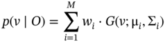
which is the sum of weighted Gaussians with unknown means and variances. The parameters wi, μi, and Σi have to be estimated using a kind of optimisation technique. Often expectation maximisation is used for this purpose [42].
9.3.7 Logistic Regression
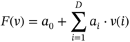
Logistic regression is generally to estimate the probability of an observation subject to an attribute. It estimates the observation probability from the given features. A logistic function F(v) is computed from the features as:

where F(v) depends on the sequence of attributes (i.e. previous experiences):
and for testing:
To give an example, consider:
- Observation O: suffering from back pain &
 : not suffering from back pain
 - Attribute ν: age:
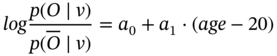
During the training stage a0 (the log odds for a 20-year-old person) and a1 (the log odds ratio when comparing two persons who differ by one year in age) are estimated. In the testing stage the probability of having back pain given the age is estimated as:
9.3.8 Reinforcement Learning
In reinforcement learning an agent learns a good behaviour. This means that it modifies or acquires new behaviours and skills incrementally [43]. It exploits the local information as well as the restrictions imposed on the WSN application to maximise the influences of numerous tasks over a time period. Therefore, during the process of reinforcement learning, the machine learns by itself based on the penalties and rewards it receives in order to decide on its next step action. Thus, the learning process is sequential. With this algorithm, each WSN node discovers the minimal needed resources to carry out its routine tasks with benefits allocated by the Q-learning technique. This technique is mainly used to assess the value or quality of action taken by the learning system (embedded in each sensor for distributed cases) for the estimation of the award to be given [44] and consequently undertaking the next step.
9.3.9 Artificial Neural Networks
ANNs are other supervised nonlinear machine learning algorithms constructed by cascading chains of decision units (neurons followed by nonlinear functions and decision-makers) used to recognise nonlinear and complex functions [10]. In WSNs, using NNs in distributed manners is still not so pervasive due to the high computational requirements for learning the network weights and the high management overhead. However, in centralised solutions, NNs can learn multiple outputs and decision boundaries at once [45], which makes them suitable for solving several network challenges using the same model.
As seen in Figure 9.6, each ANN consists of input and output layers plus a number of hidden layers. Each layer contains a number of neurons and each neuron performs a nonlinear operation on its input. Hard limiter (sign function), sigmoid, exponential, and tangent hyperbolic (tanh) functions are the most popular ones.
The major challenges in using ANNs are their optimisation (i.e. estimation of the link weights) and selection of the number of layers and neurons. Backpropagation algorithms are often used in multilayer ANNs [46, 47]. This is very similar to the optimisation of adaptive filter coefficients, where the error between the achieved label (output) and the desired label is minimised in order to obtain the best set of link weights. The computational cost exponentially increases with the numbers of neurons and layers.
In an example of NN application for WSN node localisation, the input variables are the propagating angle and distance measurements of the received signals from anchor nodes [48]. Such measurements may include received signal strength indicator (RSSI), time of arrival (TOA), and time difference of arrival (TDOA), as illustrated in Figure 9.7. After supervised training, the NN generates an estimated node location as vector-valued coordinates in 3D space. The associated NN algorithms include self-organising map (or Kohonen maps) and learning vector quantisation (LVQ) (see [49] and references therein for an introduction to these methods). In addition to function estimation, one important application of NNs is in big data (high-dimensional and complex dataset) feature detection, classification, and dimensionality reduction [50].
Using backpropagation algorithm to train an ANN, the error between the output of each output neuron is compared with a target value (or the centre of a cluster) in order to find the link weights between various layers. For the two-layer network of Figure 9.7, assuming zk is the output of neuron k and tk the target, the cost is defined as:
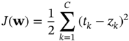
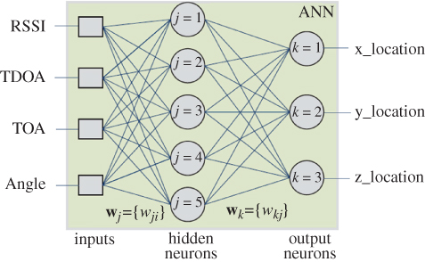
Figure 9.7 A simple three-layer NN for node localisation in WSNs in 3D space.
where C represents the number of outputs (classes). Estimation of the output, zk, is straightforward; assuming the input vector to the ANN is x, the output of neuron k is:
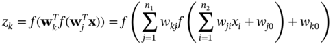
In the above equation, n1 and n2 are the number of neurons in the first and second layers respectively, wj0 and wk0 are bias values (not shown in Figure 9.7), and f (y), the neuron activation function is a continuous function which best approximates a hard limiter often called as rectified linear unit (ReLU). A popular example of such a function is the following exponential function:
which looks like the curve in Figure 9.8. Many other functions can also be used, as stated previously. Different optimisation techniques such as MSE minimisation [51] can be used to minimise J(w) and find the optimum wji and wkj values.
9.3.9.1 Deep Neural Networks
In parallel with the development of powerful computers and accessing to local and remote memory clusters as well as the cloud, DNNs have become widely popular. These classifiers often have a larger number of neurons and layers and a greater ability to learn, are more scalable, and have further processing capability on their layers. Unlike in the past, currently, large data can be processed using DNNs in real-time. Deep learning using DNNs allows computational models that are composed of multiple processing layers to learn data representations with multiple abstraction levels.
With the advancement of deep learning algorithms, developers, analysts, and decision-makers can explore and learn more about the data and their exposed relationships or hidden features. The new practices in developing data-driven application systems and decision making algorithms seek adaptation of deep learning algorithms and techniques in many application domains. In data-driven learning applications, the data govern the system behaviour.

Figure 9.8 An exponential activation function (ReLU).
The availability of deep structure as well as data-driven models paves the path for developing a new generation of deep networks called generative models. Unlike discriminative networks, which estimate a label for a test data, the generative networks assume they have the class label, and they wish to find the likelihood of particular features. They are often called generative adversarial networks (GANs) and include two nets, pitting one against the other (thus the ‘adversarial’). GANs were introduced by Goodfellow et al. [52] and were called the most interesting idea in machine learning in the last 10 years be LeCun, Facebook's AI research director.
In GANs, the generative models are designed via an adversarial process, in which two models are trained simultaneously: a generative model G that captures the data distribution, and a discriminative model D that estimates the probability that a sample is taken from the training data rather than G. To train the G model the probability of D making a mistake is maximised. This framework resembles a minimax two-player game. For arbitrary functions G and D, a unique solution exists, with G recovering the training data distribution and D equal to 0.5 everywhere. In the case where G and D are defined by multilayer perceptrons, the entire system can be trained with a backpropagation algorithm [52].
One particular type of deep feedforward network is the convolutional neural network (CNN) [53, 54]. This network is easier to train and can generalise much better than networks with full connectivity between adjacent layers. It often performs better in terms of both speed and accuracy for many computer vision and video processing applications. Recently, CNNs have found many other applications, such as for the detection of interictal epileptiform discharges from intracranial EEG recordings [55, 56].
9.3.9.2 Convolutional Neural Networks
CNNs are designed to process multiple array data such as colour images composed of three 2D arrays containing pixel intensities in the three colour channels. These networks have four main features that benefit from the properties of natural signals, namely local connections, shared weights, pooling, and the use of numerous layers. Typical CNN architecture is structured as a series of stages (Figure 9.9). The first few stages are composed of two types of layers: convolutional layers and pooling layers. Units in a convolutional layer are organised in feature maps, within which each unit is connected to local patches in the feature maps of the previous layer through a set of weights called a filter bank. The result of this local weighted sum is then passed through a nonlinearity such as an ReLU. All units in a feature map share the same filter bank. In a conventional CNN different feature maps in a layer use different filter banks. The reason for this architecture is twofold. First, in array data such as images, local groups of values are often highly correlated, forming distinctive local motifs that are easily detected. Second, the local statistics are invariant to location. In other words, if a motif can appear in one part of the image, it may appear anywhere in the image. Hence, we can have units at different locations sharing the same weights and detecting the same pattern in different parts of the array. From a mathematical point of view, the filtering operation performed by a feature map is a discrete convolution, hence the name.
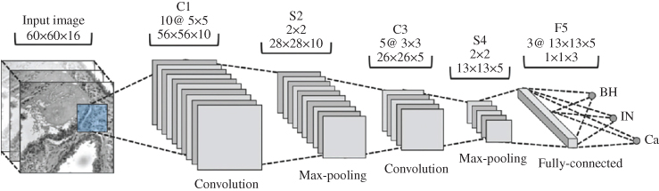
Figure 9.9 An example of a CNN and its operations.
Although the role of a convolutional layer is to detect local conjunctions of features from the previous layer, the role of the pooling layer is to merge semantically similar features into one. Since the relative positions of the features forming a motif can vary somewhat, its reliable detection can be performed by coarse-graining the position of each feature. A typical pooling unit computes the maximum of a local patch of units in one feature map (or in a few feature maps).
The neighbouring pooling units take input from patches that are shifted by more than one row or column, thereby reducing the representation dimension and creating an invariance to small shifts and distortions.
Stages of convolution, nonlinearity, and pooling are followed by more convolutional and fully connected layers. The backpropagation operation is then used for weight optimisation in a CNN as for the normal multilayer NN.
DNNs exploit the property that many natural signals follow compositional hierarchies. Based on this property, the higher-level features are obtained by composing lower-level ones. In images, local combinations of edges form motifs, motifs assemble into parts, and parts form objects. Similar hierarchies exist in speech and text from sounds to phones, phonemes, syllables, words, and sentences. The pooling allows representations to vary very little when elements in the previous layer vary in position and appearance.
The convolutional and pooling layers in CNNs are directly inspired by the classic notions of simple cells and complex cells in visual neuroscience [54], and the overall architecture is reminiscent of the LGN–V1–V2–V4–IT hierarchy (where LGN stands for lateral geniculate nucleus) in the visual cortex ventral pathway [57].
When the CNN models and monkeys are projected/shown the same picture, the activation of high-level units in the CNN explains half of the variance of random sets of 160 neurons in the monkeys' inferotemporal cortex [58]. CNNs have their roots in the neocognitron [59], the architecture of which is somewhat similar, but does not have an end-to-end supervised-learning algorithm such as backpropagation. Although CNNs were initially developed for image classification, an effective 1D CNN was developed by Antoniades et al. [55, 56] for the detection of interictal epileptiform discharges from intracranial EEG recordings.
9.3.9.3 Recent DNN Approaches
One of the early introduced DNNs was LeNet proposed by LeCun in 1988 for hand digit recognition [60]. LeNet is a feed-forward NN constituted of five consecutive layers of convolutional and pooling, followed by two fully connected layers. A later DNN approach was AlexNet [61]. This approach, proposed by Krizhevsky et al., is considered the first deep CNN architecture which showed ground-breaking results for image classification and recognition tasks.
Learning mechanism of CNN was largely based on hit-and-trial, without a deep understanding of the exact reason behind the improvement before 2013. This lack of understanding limited the performance of deep CNNs on complex images. In 2013, Zeiler and Fergus [62] proposed a multilayer deconvolutional NN (DeconvNet), which became known as ZefNet to quantitatively visualise the network performance.
A deeper network, namely visual geometry group (VGG), was later proposed [63]. VGG suggested that the parallel placement of small size filters makes the receptive field as effective as that of large size filters. GoogleNet (also known as Inception-V1) is another CNN which won the 2014-ILSVRC (ImageNet Large-Scale Visual Recognition Challenge) competition [64]. The main objective of the GoogleNet architecture was to achieve high accuracy with a reduced computational cost. It introduced the new concept of inception module (block) in CNN, whereby multiscale convolutional transformations are incorporated using split, transform, and merge operations for feature extraction. Other deep networks such as ResNet [65], DenseNet [66], and many other DNN structures were later introduced for enhancing the accuracy of feature learning and classification.
In large NNs, model pruning seeks to induce sparsity in a DNN's various connection matrices, thereby reducing the number of nonzero-valued parameters in the model. Weights in an NN that are considered unimportant or rarely fire can be removed from the network with little or no consequence. Often, many neurons have a relatively small impact on the model performance, meaning we can achieve acceptable accuracy even when eliminating a large number of parameters. Reducing the number of parameters in a network becomes increasingly important as neural architectures and datasets becoming larger in order to obtain reasonable execution times of models.
Among NNs, recurrent neural networks (RNNs) and long short-term memory network (LSTM) rely on their previous states and therefore can learn state transitions for detection or recognition of particular/desired trends within the data. RNNs can be also used for prediction purposes. A shallow RNN, however, is not capable of using long-term dependencies between the data samples. LSTMs are a special kind of RNNs, which are capable of learning long-term dependencies. They were introduced by Hochreiter and Schmidhuber [67] and were refined and popularised by many people, such as Xu et al. [68]. Unlike RNN, which has only a single layer in each repeating module, the repeating module in an LSTM contains four interacting layers. A similar idea has been followed and explored for speech data generation. WaveNet DNN, as a probabilistic and autoregressive DNN approach, has been designed and applied for speech waveform generation [69]. This architecture exploits the long-range temporal dependencies needed for raw audio generation.
Despite heavy DNN computational cost, some DNN structures such as ENet (efficient neural network), have been proposed to enable real-time applications. ENet, meant for spatial classification and segmentation of images, uses a significantly smaller number of parameters.
9.3.10 Gaussian Processes
Gaussian processes (GPs) [70] are other algorithms for solving regression and probabilistic classification problems. These supervised classifiers, though not effective for large dimension data, use prediction to smooth the observation and are versatile enough to use different kernels. Therefore, they are suitable for recovering and classifying biomedical signals which often have a regular structure.
The GP approach performs inference using the noisy, potentially artefactual, data obtained from wearable sensors. Of fundamental importance is the GP notion as a distribution over functions, which is well suited to the analysis of the time series of patients' physiological data, in which the inference over functions may be performed. This approach contrasts with conventional probabilistic approaches which define distributions over individual data points.
As an example, a GP was used in an e-health platform for personalised healthcare to develop a patient-personalised system for the analysis and inference in the presence of data uncertainty [71]. This uncertainty is typically caused by sensor artefact and data incompleteness. The method was used for the clinical study and monitoring of 200 patients [71]. This provides the evidence that personalised e-health monitoring is feasible within an actual clinical environment, at scale, and that the method is capable of improving patient treatment outcome via personalised healthcare.
In another example a Bayesian Gaussian process logistic regression (GP-LR) with linear and nonlinear covariance functions has been used for the classification of Alzheimer's disease and mild cognitive impairment from resting-state fMRI [72]. These models can be interpreted as a Bayesian probabilistic system analogue to kernel SVM classifiers. However, GP-LR methods confer some benefits over kernel SVMs. Whilst SVMs only return a binary class label prediction, GP-LR, being a probabilistic model, provides a principled estimate of the probability of class membership. Class probability estimates are a measure of confidence the model has in its predictions. Such a confidence score can be very useful in the clinical setting.
9.3.11 Neural Processes
Garnelo et al. [73] introduced a class of neural latent variable models, namely neural processes (NPs), by combining GPs and NNs. Like GPs, NPs define distributions over functions, are capable of rapid adaptation to new observations, and can estimate the uncertainty in their predictions. Like NNs, NPs are computationally efficient during training and evaluation but also learn to adapt their prior probability distributions.
NPs perform regression by learning to map a context set of observed input–output pairs to a distribution over regression functions. Each function models the distribution of the output given an input, conditioned on the context. NPs have the benefit of fitting observed data efficiently with linear complexity in the number of context input–output pairs. They are able to learn a wide family of conditional distributions; they learn predictive distributions conditioned on context sets of arbitrary size.
Nonetheless, it has been shown that NPs suffer underfitting, giving inaccurate predictions at the inputs of the observed data they condition on [74]. This problem has been addressed by incorporating attention into NPs, allowing each input location to attend to the relevant context points for the prediction. It has been shown that this greatly improves the accuracy of predictions, speeds up the training process, and expands the range of functions that can be modelled [74].
9.3.12 Graph Convolutional Networks
Graph convolutional networks (GCNs) are powerful NNs which enable machine learning on graphs. Even small-size GCNs can produce useful feature representations of nodes in the network. In a GCN structure, the relative proximity of the network nodes is preserved in the 2D representation even without any training. There are two different inputs to a GCN: one is the input feature matrix and the other a matrix representation of the graph structure, such as the adjacency matrix of the graph. As an example, consider the classification of EEG signals for healthy and dementia subjects. Using a GCN, the brain connectivity estimates can be incorporated into the training process as the proximity matrix.
As an example, for a two-layer GCN the following relation between the input and output can be realised [75]:
where A is the adjacency matrix, ![]() ,
, ![]() , IN is an N × N identity matrix, and
, IN is an N × N identity matrix, and ![]() .
.
9.3.13 Naïve Bayes Classifier
Naïve Bayes classification method is a supervised learning algorithm applying Bayes' theorem with the ‘naïve’ assumption of independence between every pair of features. Therefore, the class label of the data can be estimated using a naïve Bayes classifier through the following procedure.
Given a class variable y and a dependent feature vector x1 through xn, the Bayes theorem states the following relationship:

Using the naïve independence assumption:
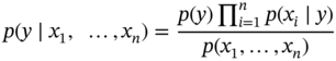
Since p(x1, …, xn) is constant for any given input, the following classification rule can be deduced:
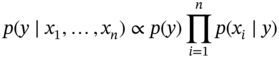
The likelihood probability p(xi ∣ y) is considered known either empirically or by assumption. Gaussian, multinomial, and Bernoulli are among the most popular distributions considered for these probabilities. This results in estimation of a class label as:
Naïve Bayes classifiers are simple and work quite well in many real-world situations. They require a small selection of training data to estimate the necessary parameters [76].
Naïve Bayes learners and classifiers can be extremely fast compared to more computationally intensive methods. The decoupling of the class conditional feature distributions means that each distribution can be independently estimated as a 1D distribution. This in turn helps alleviate the problem of the curse of dimensionality.
9.3.14 Hidden Markov Model
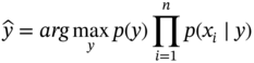
HMMs are state-space machines meant to detect a correct data sequence which may happen within a longer data sequence. HMMs are presented as the state diagrams. Therefore, for each application, an HMM has a certain number of states and knows the probability of each possible event happening in each state. As an example, consider the detection of QRS in an electrocardiogram (ECG) signal depicted in Figure 9.10.
From this figure, an ECG is recognised when the symbols turn up in a correct sequence in the signal. Assuming the waveform in Figure 9.10 is the ECG of a healthy subject, the state diagram in Figure 9.11 classifies the subject as healthy as long as the above ECG sequence is detected in his/her ECG record.
In this diagram, state Q0 is a wait state to detect the beginning of sequence starting from a bar (b). State Q1 is a state which shows a bar has been detected. State Q2 simply demonstrates that a bar and a small hump (p) have been already recognised. Q3 represents the state of the system when a bar, a small hump, and a QRS wave are correctly sequenced. Q4 and Q5 similarly show the states after a bar and a large hump (t) have been respectively added to the data sequence. After detecting the correct sequence, the output is ‘the subject is healthy’. After each state, if a wrong symbol or noise is detected, the system output is ‘the subject is not healthy’.
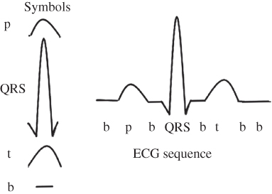
Figure 9.10 A synthetic ECG segment of a healthy individual and its corresponding symbols.
Figure 9.11 An HMM for the detection of a healthy heart from an ECG sequence.
In places where the objective is to detect a particular heart condition, separate HMM should be designed to recognise that condition. Beside their applications in biomedical signal analysis and disease recognition, HMMs have a wide range of applications in speech, video, bioscience (such as genomics), and face recognition.
In order to use an HMM for classification, the initial state (π = πi, where i = 1, …, N, where N is the number of states), the state probabilities (A = {aij}, i,j = 1, …, N), and the state transition probabilities (B = {bj(k)}, j = 1, …, N, k = 1, …, T, where T is the observation sequence length) should be known. For training the HMMs (i.e. to find the model parameters), however, a set of observations and the number of states should be known.
There are three major problems (objectives) in using or designing HMMs:
- Given the observation sequence O = o1, o2, …, oT, and the model λ = (A, B, π), what will be the probability of observation sequence p(O|λ)?
- Given the observation sequence and the model as above, how can we find the state sequence Q = Q1, …, QN which generates such an observation sequence?
- Given the observations and the number of states, how can the HMM model be built up, i.e. how can we find λ = (A, B, π)?
To solve the first problem, often, the iterative forward–backward algorithm is used, while the Viterbi algorithm is employed to solve the second problem. Finally, quite a few algorithms, such as the most popular one, Baum–Welch (Leonard E. Baum and Lloyd R. Welch, 1960s) [77, 78], can be used to solve the third problem which is the most important one.
To go through forward–backward algorithms, set λ = (A, B, π) with random initial conditions (unless some information about the parameters is available already). Then, follow the iterative procedures below.
9.3.14.1 Forward Algorithm
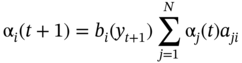
Let αi(t) = p(o1 = y1, …ot = yt, Qt = i ∣ λ) the probability of observing y1, y2, …, yt and being in state i at time t.
and iterate over t:
9.3.14.2 Backward Algorithm
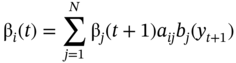
Let βi(t) = p(ot + 1 = yt + 1, …, oT = yT, Qt = i ∣ λ) the probability of observing yt+1, y2, …, yT partial sequence and being in state i at time t.
and iterate over t:
9.3.14.3 HMM Design
For HMM design we need to calculate the following auxiliary variables following the Bayes theorem:
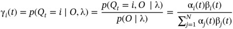
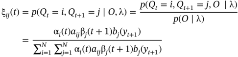
This is the probability of being in state i at time t for a given model λ and the observed sequence O. Then, the probability of being in states i and j at times t and t + 1, respectively, for the given model λ and the observed sequence O is:
The HMM parameters for the model λ are then updated using:
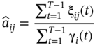
p(O|λ) is then calculated utilising these parameters. After each iteration, this probability increases until the parameters A, B, and π reach their optimum values, where the algorithm terminates and there won't be any considerable change in the probability.
9.4 Common Spatial Patterns
The common spatial pattern (CSP) is a popular feature extraction and optimisation method for the classification of multichannel signals (such as EEG). CSP aims to estimate spatial filters which discriminate between two classes based on their variances. CSP (w) minimises the Rayleigh quotient of the spatial covariance matrices to achieve the variance imbalance between two classes of data, X1 and X2. Before applying CSP, the signals are bandpass filtered and centred. The CSP goal is to find a spatial filter w∈ℜc such that the variance of the projected samples of one class is maximised while the other's is minimised. The following maximisation criterion is used for CSP estimation [79, 80]:

where C1 and C2 are covariance matrices of the two clusters X1 and X2 and tr refers to trace of a matrix. With k as any real constant, this optimisation problem can be solved (though this is not the only way) by first observing that the function J(w) remains unchanged even if the filter w is rescaled, i.e. J(kw) = J(w), Hence, extremising J(w) is equivalent to extremising wTC1w subject to the constraint wTC2w = 1, since it is always possible to find a rescaling of w such that wTC2w = 1. Employing Lagrange multipliers, this constrained problem changes to an unconstrained problem as [81]:
A simple way to derive optimum w is to take derivatives of L and set to zero as follows:
Based on the standard eigenvalue problem, spatial filters extremising Eq. (9.54) are then the eigenvectors of ![]() corresponding to its largest and lowest eigenvalues. When using CSP, the extracted features are derived from logarithm of the signal variance after projection to filters w.
corresponding to its largest and lowest eigenvalues. When using CSP, the extracted features are derived from logarithm of the signal variance after projection to filters w.
Eigenvalue λ measures the ratio of variances of the two classes. CSP is suitable for classification of both spectral [80] and spatial data since power of the latent signal is larger for the first cluster than for the second cluster.
Applying this approach to separation of event-related potentials (ERPs) from EEG signals enhances one of the classes against the rest. This allows a better discrimination between the two classes, thus can be separated easier.
In early 2000 in a two-class BCI setup, Ramoser et al. [82] proposed the application of CSP that learnt to maximise the variance of bandpass filtered EEG signals from one class while minimising their variance from the other class. Currently, CSP is widely used in BCI where evoked potentials or movement can cause alteration of signals.
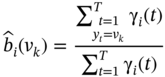
The model uses the four most important CSP filters. The variance is then calculated from the CSP time series. Then, a log operation is applied and the weight vector obtained with the LDA is used to discriminate between left- and right-hand movement imaginations. Finally, the signals are classified and based on that an output signal is produced to control the cursor on computer screen. Patterns related to right-hand movement are shown in Figure 9.12a and those for left-hand movement in Figure 9.12b. These patterns are the strongest patterns.
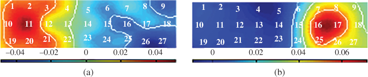
Figure 9.12 CSPs related to right-hand movement (a) and left-hand movement (b). The EEG channels are indicated by numbers that correspond to three rows of channels (electrodes) within the central and centroparietal regions. (See color plate section for color representation of this figure)
Most of the existing CSP-based methods exploit covariance matrices on a subject-by-subject basis so that the inter-subject information is neglected. In that paper, CSP has been modified for subject-to-subject transfer, where a linear combination of covariance matrices of subjects under consideration has been exploited. Two methods have been developed to determine a composite covariance matrix that is a weighted sum of covariance matrices involving subjects, leading to composite CSP [83].
The accurate estimation of CSPs under weak assumptions (mainly noisy cases) requires derivation of an asymptotically optimal solution. This in sequel necessitates calculation of the loss in signal-to-noise-plus-interference ratio because of the finite sample effect in a closed form. This is often important in the detection/classification of ERPs since the EEG or magnetoencephalography (MEG) signals contains not only the spatiotemporal patterns bounded to the events but also ongoing brain activity as well as other artefacts such as eye blink and muscle movement artefacts. Therefore, to improve the estimation results CSPs are applied to the recorded multichannel signals.
In Eq. (9.54), the trace values are equivalent to L2-norm. Owing to the sensitivity of L2-norm to outliers [84], it is replaced by L1-norm. This changes Eq. (9.54) to:
where m and n are the total sampled points of the two classes and ‖·‖1 refers to the L1-norm. It has been shown that, using this approach, the effects of outliers are alleviated.
Most of the existing CSP-based methods exploit covariance matrices on a subject-by-subject basis so that inter-subject information is neglected. CSP and its variants have received much attention and have been one of the most efficient feature extraction methods for BCI. However, despite its straightforward mathematics, CSP overfits the data and is highly sensitive to noise.
To enhance CSP performance and address these shortcomings, recently it has been proposed to improve the CSP learning process using prior information in the form of regularisation terms or constraints. Eleven different regularisation methods for CSP have been categorised and compared by Lotte and Guan [81]. These methods included regularisation in the estimation of the EEG covariance matrix [85], composite CSP [83], regularised CSP with generic learning [86], regularised CSP with diagonal loading [80], and invariant CSP [87]. All the algorithms were applied to a number of trials from 17 subjects and the CSP with Tikhonov regularisation in which the optimisation of J(w) was penalised by minimising ||w||2, and consequently minimising the influence of artefacts and outliers, was suggested as the best method.
To make CSP less sensitive to noise, the objective function in (9.57) may be regularised either during estimation of the covariance matrix for each class or during the minimisation process of the CSP cost function by imposing priors to the spatial filters w [81]. A straightforward approach to regularise the estimation of the covariance matrix for class i, i.e. ![]() , is denoted as:
, is denoted as:
where P is estimated as:
In these equations, Ci is the initial spatial covariance matrix for class i, Gi, the so-called generic covariance matrix, is computed by averaging the covariance matrices of a number of trials for class i, though it may be defined based on neurophysiological priors only, and γ and β ∈ [0,1] are the regularising parameters. The generic matrix represents a given prior on how the covariance matrix for the mental state considered should be.
In regularising the CSP objective function on the other hand, a regularisation term is added to the CSP objective function in order to penalise the resulting spatial filters that do not satisfy a given prior. This results in a slightly different objective function as [81]:
The penalty function Q(w) weighted by the penalty (or Lagrange) parameter α ≥ 0 indicates how much the spatial filter w satisfies a given prior. Similar to the first term in the denominator of (9.60), this term needs to be minimised in order to maximise the cost function J(w). In the literature, different quadratic and nonquadratic penalty functions have been defined. Some exemplar methods can be seen in [81, 87, 88]. A quadratic constraint, such as Q(w) = wTKw, results in solving a new set of eigenvalue problems as [81]:
The composite CSP algorithm proposed in [83] performs subject-to-subject transfer by regularising the covariance matrices using other subjects' data. In this approach α and γ are zero and only β is nonzero. The generic covariance matrix Gi is defined according to the covariance matrices of other subjects.
The approach based on regularised CSP with generic learning [86] uses both β and γ regularisation terms, which means it intends to shrink the covariance matrix towards both the identity matrix and a generic covariance matrix Gi. Here, similar to composite CSP, Gi is computed from the covariance matrices of other subjects.
Diagonal loading (DL) is another form of covariance matrix regularisation used in BCI literature [80], which consists of shrinking the covariance matrix towards the identity matrix (sometimes called orthonormalisation). Hence, in this approach, only γ is used (α = β = 0) and its value can automatically be identified using Ledoit and Wolf's method [86] or by cross-validation [81].
In the approach based on Tikhonov regularisation [81], the penalty term is defined as P(w) = ||w||2 = wTw = wTI w which is obtained by using K = I in (9.61a and b). Such regularisation is expected to constrain the solution to filters with a small norm, hence mitigating the influence of artefacts and outliers.
Finally, in the weighted Tikhonov regularisation method, it is considered that some EEG channels are more important than others (as expected). Therefore, signals from these channels are weighted more than those of others. This consequently causes different penalisations for different channels. To perform this regularisation method, define P(w) = wTDww, where Dw is a diagonal matrix whose entries are defined based on the measures of CSPs from other subjects [81].
The obtained results in implementing 11 different regularisation methods in [81] show that in places where the data are noisy the regularisation improves the results by approximately 3% on average. However, the best algorithm outperforms CSP by about 3–4% in mean classification accuracy and by almost 10% in median classification accuracy. The regularised methods are also more robust, i.e. they show lower variance across both classes and subjects. Among various approaches, the weighted Tikhonov regularised CSP proposed in [81] has been reported to have the best performance.
Regularisation of w can also be used to reduce the number of EEG channels without compromising the classification score. Farquhar et al. [87] converted CSP into a quadratically constrained quadratic optimisation problem with l1-norm penalty and Arvaneh et al. [89] used l1/l2-norm constraint. Recently, in [90] a computationally expensive quasi l0-norm-based principle was applied to achieve a sparse solution for w. In [83] CSP was modified for subject-to-subject transfer, to exploit a linear combination of covariance matrices of subjects under study. In this approach a composite covariance matrix, i.e. a weighted sum of covariance matrices involving subjects, was used, leading to composite CSP.
9.5 Applications of Machine Learning in BSNs and WSNs
Numerous applications for most of the machine learning methods above have been briefly explained in the related sections. A few more examples are as follows.
9.5.1 Human Activity Detection
Physical and mental disabilities highly affect the human posture and movements during daily life. Measurements from a single sensor, the fusion of data from multiple body sensors [91], and the analysis of the data from distributed body sensors [92] have been practiced recently. Accelerometers with wireless transmission system have been the most popular sensors in many recent applications.
Most existing works proposed in [93–102] are based on off-line processing systems to perform gesture or activity recognition. There are some recent works focusing on real-time activity recognition. Tapia et al. [103] propose a real-time DT-based algorithm for recognition of physical activities (i.e. gestures). Three-axis accelerometer sensors transmit the information wirelessly to a laptop computer for processing.
A tree-based classifier is initially trained and then used to recognise gymnasium activities in real time. Krishnan et al. [104] propose an AdaBoost algorithm based on decision stumps for real-time classification of gestures (i.e. walking, sitting, and running) using three-axis accelerometer sensors. He et al. [105] present an HMM-based approach for real-time activity classification using acceleration data collected from a wearable WSN. The model is used to classify a number of gestures such as standing, sitting, and falling.
Wang et al. [91] propose a real-time, hierarchical model to recognise both simple gestures and complex activities using a wireless body sensor network (WBSN). In this model, they initially employed a fast, lightweight template matching algorithm to detect gestures at the sensor node level, and then used a discriminative pattern based real-time algorithm to recognise high-level activities at the portable device level.
Györbíró et al. [106] present a real-time mobile activity recognition system consisting of wireless body sensors, a smartphone, and a desktop workstation. A sensor node has an accelerometer, a magnetometer, and a gyroscope. They propose a recognition model based on feed-forward backpropagation NNs which are first trained at a desktop workstation, and then run at the smartphone to recognise six different gestures. Liu et al. [107] propose an efficient gesture recognition method based on a single accelerometer using dynamic time warping (DTW). They first defined a vocabulary of known gestures based on training, then used these predefined templates for recognising hand gestures.
Yang et al. [92] propose a distributed recognition framework to classify continuous human actions using a low-bandwidth wearable motion sensor network, called distributed sparsity classifier (DSC). The algorithm classifies human actions using a set of training motion sequences as prior examples. It is also capable of rejecting outlying actions that are not in the training categories. The classification is operated in a distributed fashion on individual sensor nodes and a computer base station. The distribution of multiple action classes is modelled as a mixture subspace model, one subspace for each action class. Given a new test sample, the method seeks the sparsest linear representation of the sample versus all the training examples. It has been shown that the dominant coefficients in the representation only correspond to the action class of the test sample, and hence its membership is encoded in the sparse representation.
Lombriser et al. [108] used a set of wireless accelerometers, light sensors, and a microphone to recognise the office daily activities such as drinking water, moving a computer, mouse writing on a whiteboard, opening a drawer, opening a cupboard, typing on a keyboard, and writing with a pen. They used kNN and DT classifiers and demonstrated a recognition rate of above 90%.
Ravi et al. [109] used DNN for recognition of activities of daily living. In their approach they use the spectrogram of an inertial signal, as a function of frequency and time. The convolution filters are then applied to the spectrogram vertically. The achieved temporal convolutions produce an output layer of the learnt network from small segment features, enabling real-time processing. This provides orientation invariance to the input signal. Finally, the last two layers are used to classify the features. They applied their algorithm on a number of standard datasets and report over 95% correct classification rates.
9.5.2 Scoring Sleep Stages
Prochazka et al. [110] show that the sleep stages can be classified and scored from multiple sensor polysomnography (PSG), including EEG, ECG, oximeter, and breathing information, data up to a very high accuracy. They effectively used multimodal data features in time and frequency for this purpose. They compared the results of applying DT, NNs, and SVMs to classify and score sleep stages. In this analysis time-frequency and time-scale features have been used [111].
9.5.3 Fault Detection
Machine learning techniques have also been widely used in WSNs for environmental and industrial monitoring, mainly for human welfare. In sensor networks, fault detection in both the system itself and the recorded data is important. In WSNs the collected data are prone to the faults which often happen in either the sensors, communication links, communication systems, or the energy supply, and are due to internal and external influences [112]. The authors in [113] focus on occurring faults due to low battery and calibration in WSNs. They used HMM to identify and classify various types of faults. Offset fault, gain fault, stuck-at fault, calibration problem, and low battery have been the major faults considered in a sensor network and an HMM has been trained for each fault separately. An average accuracy of 90% has been reported in their paper.
9.5.4 Gas Pipeline Leakage Detection
In [114] SVM, kNN, GMM, and naïve Bayes machine learning techniques have been used for large gas pipeline leakage detection and size estimation through WSNs. A number of pressure sensors collect the data from different positions across normal pipes and those with low, medium, and severe leakages. Various order statistics have been estimated and utilised as the features. It has been concluded that kNN and SVM outperform others for this application [114].
9.5.5 Measuring Pollution Level
In [115] the researchers present the results of application of CNN to detect the level of pollution using the data collected from 72 metal-oxide gas sensors. In addition, they include the air purifying fan speed information proportional to the degree of air pollution. The purpose of this work is to determine the optimal fan speed for air purification in a tunnel by analysing the degree of air pollution.
In their experiment, each sensor has been used as a feature to construct a vector composed of 72 features. The value of the feature is an integer value representing the air gas value and each feature vector has a fan speed as a class. Thirty classes of speed have been used. The accuracy of fan speed prediction has also been optimised. An average prediction accuracy of approximately 85% has been reported.
9.5.6 Fatigue-tracking and Classification System
The Neuro-Fuzzy Fatigue-Tracking and Classification System for Wheelchair Users was developed by Li et al. [116]. A neuro-fuzzy fatigue tracking and classification system has been proposed and deployed for the classification of fatigue severity of wheelchair users. In the proposed system, physiological, and kinetic data are collected, including surface electromyography (EMG), ECG, and acceleration signals. The relevant features are then extracted from the signals and integrated with a self-rating method to train the neuro-fuzzy classifier. The musculoskeletal disorders caused by underlying fatigue have been recognised using various degrees of fatigue measures.
These are only a very small number of machine learning applications. Many more applications are reported in the literature and some of them are addressed in the corresponding sections of this book.
9.5.7 Eye-blink Artefact Removal from EEG Signals
In [117] and [118] SVM has been combined with blind source separation (BSS) to separate and eliminate the eye-blink artefacts from multichannel EEG signals. BSS separates the multichannel signals into their constituent independent components and SVM recognises the components belonging to eye-blinks using some simple input features related to the morphology of eye-blink signatures within EEGs. This method is very simple, effective, and accurate.
9.5.8 Seizure Detection
One of the popular subjects in EEG analysis is detection of onset of seizure for epileptic patients. One way to do that is to characterise the morphology of the seizure EEG pattern mainly in terms of amplitude, frequency range, and the decline in frequency over the seizure onset duration. These features can then be classified into seizure and non-seizure segments. SVM has been used as the classifier for this purpose in [119].
9.5.9 BCI Applications
Brain-computer interfacing (BCI) is perhaps the most popular application of machine learning. Classification of the brain motor activity, mainly from the EEG signals, is important in understanding various body part movements and also detection of an intention to move the body part. In [120] the authors have shown that temporo-spatial EEG features can be accurately used by an SVM for detection of left and right hand movements.
9.6 Conclusions
In this chapter, the most popular machine learning methods and their applications for clustering or classification of signals and information collected by BSNs have been briefly introduced. Some machine learning algorithms have less sensitivity to noise and outliers. These artefacts often make the classifier applications less reliable. Nonlinear techniques and regression-based algorithms are becoming more popular due to their advantages in classification of nonlinearly separable data. New approaches in deep learning are capable of handling nonseparable and nonlinear cases of very large datasets.
The trained large deep networks may be partially reused for the classification of data of a different nature through transfer learning [121]. Following this approach part of the network parameters may be kept fixed and the remaining final layers trained using the new data.
In places where the training data size is limited, the generation and application of surrogate data may boost the quality/accuracy of the results. In such cases, the classifiers should deal with the data distribution and statistics rather than the data samples. This is mainly because the methods for the generation of surrogate data are able to generate new data with same distribution as the data distribution. The surrogate data may not look like the data themselves. In the field of deep networks, one option is to use variational AE, which uses data distribution for learning [122].
Distributed and cooperative learning may become more popular in the near future due to the availability of on-sensor processing and decision making as well as the nature of multisensor scenarios and the large data size. Often, signal processing methods boost machine learning techniques as they can extract and provide more meaningful data features prior to machine learning applications. On the other hand, the need for on-board classification and state recognition requires many algorithms to be developed in Python, Java, and machine languages suitable for compact wearable devices, tablets, and mobile phones.
Moreover, real-time applications require faster systems which are able to process, communicate, and make decisions within one sample interval. Many regression-based classifiers can cope with real-time applications. In the area of DNN, a deep reinforcement learning approach has been claimed to be able to perform real-time learning classification [123]. Nevertheless, these networks need considerable time for training.
References
- 1 Akcay, S., Atapour-Abarghouei, A., and Breckon, T. P. (2018). GANomaly: semi-supervised anomaly detection via adversarial training. arXiv:1805.06725.
- 2 Sanei, S. (2013). Adaptive Processing of Brain Signals. Wiley.
- 3 Fu, L. and Medico, E. (2007). FLAME: a novel fuzzy clustering method for the analysis of DNA microarray data. BMC Bioinformatics 8 (3).
- 4 Vapnik, V. (1998). Statistical Learning Theory. Wiley Press.
- 5 Paradis, L. and Han, Q. (2007). A survey of fault management in wireless sensor networks. Journal of Network and Systems Management 15 (2): 171–190.
- 6 Krishnamachari, B., Estrin, D., and Wicker, S. (2002). The impact of data aggregation in wireless sensor networks. In: 22nd International Conference on Distributed Computing Systems Workshops, 575–578.
- 7 Al-Karaki, J. and Kamal, A. (2004). Routing techniques in wireless sensor networks: a survey. IEEE Wireless Communications 11 (6): 6–28.
- 8 Romer, K. and Mattern, F. (2004). The design space of wireless sensor networks. IEEE Wireless Communications 11 (6): 54–61.
- 9 Wan, J., Chen, M., Xia, F. et al. (2013). From machine-to-machine communications towards cyber-physical systems. Computer Science and Information Systems 10: 1105–1128.
- 10 Bengio, Y. (2009). Learning deep architectures for AI. Foundations and Trends in Machine Learning 2 (1): 1–127.
- 11 Hoffmann, A.G. (1990). General limitations on machine learning. In: European Conference on Artificial Intelligence, 345–347. ECAI.
- 12 Kouchaki, S., Yang, Y., Walker, T.M. et al. (2019). Application of machine learning techniques to tuberculosis drug resistance analysis. Bioinformatics 35 (13): 2276–2282. https://doi.org/10.1093/bioinformatics/bty949.
- 13 Hartigan, J. and Wong, M. (1979). A k-means clustering algorithm. Applied Statistics 28: 100–108.
- 14 Fellous, J.-M., Tiesinga, P.H.E., Thomas, P.J., and Sejnowski, T.J. (2004). Discovering spike patterns in neural responses. Journal of Neuroscience 24 (12): 2989–3001.
- 15 Hastie, T., Tibshirani, R., and Walter, G. (2000) Estimating the number of clusters in a dataset via the gap statistic. Tech. Rep. 208, Stanford University, Stanford, CA.
- 16 Ester, M., Kriegel, H.-P., Sander, J., and Xu, X. (1996). A density-based algorithm for discovering clusters in large spatial databases with noise. In: KDD-96 Proceedings, 226–231. AAAI.
- 17 Ng, Y.A., Jordan, M.I., and Weiss, Y. (2002). On spectral clustering: analysis and an algorithm. In: Conference on Neural Information Processing Systems. MIT Press.
- 18 Ioffe, S., Szegedy, C. (2015). Batch normalization: accelerating deep network training by reducing internal covariate shift, arXiv:1502.03167.
- 19 Lin, F. and Cohen, W.W. (2010). Power iteration clustering. In: Proceedings of the 27th International Conference on Machine Learning, ICML 2010, 655–666. Omnipress.
- 20 Rasmus, A., Mikko Honkala, V., Berglund, M., and Raiko. T. (2015) Semi-supervised learning with ladder networks, arXiv:1507.02672 [cs.NE].
- 21 Bair, E. (2013). Semi-supervised clustering methods. Wiley Interdisciplinary Reviews: Computational Statistics 5 (5): 349–361.
- 22 Bezdek, J.C. (1981). Pattern Recognition with Fuzzy Objective Function Algorithms. Springer.
- 23 Ayodele, T.O. (2010). Types of machine learning algorithms. In: New Advances in Machine Learning (ed. Y. Zhang). InTechOpen https://doi.org/10.5772/9385.
- 24 Safavian, S.R. and Landgrebe, D. (1991). A survey of decision tree classifier methodology. IEEE Transactions on Systems, Man and Cybernetics 21 (3): 660–674.
- 25 Lu, C.-H. and Fu, L.-C. (2009). Robust location-aware activity recognition using wireless sensor network in an attentive home. IEEE Transactions on Automation Science and Engineering 6 (4): 598–609.
- 26 Breiman, L. (2001). Random forests. Machine Learning 45: 5–32.
- 27 Vapnik, V. (1995). The Nature of Statistical Learning Theory. New York: Springer.
- 28 Bennet, K.P. and Campbell, C. (2000). Support vector machines: hype or hallelujah? ACM SIGKDD Explorations Newsletter 2 (2): 1–13.
- 29 Christianini, N. and Shawe-Taylor, J. (2000). An Introduction to Support Vector Machines. Cambridge University Press.
- 30 DeCoste, D. and Scholkopf, B. (2001). Training invariant support vector machines. Machine Learning 46: 161–190.
- 31 Burges, C. (1998). A tutorial on support vector machines for pattern recognition. Data Mining and Knowledge Discovery 2: 121–167.
- 32 Gunn, S., (1998) Support vector machines for classification and regression. Technical Reports, Dept. of Electronics and Computer Science, Southampton University. http://ce.sharif.ir/courses/85-86/2/ce725/resources/root/LECTURES/SVM.pdf (accessed 25 November 2019).
- 33 Chapelle, O. and Vapnik, V. (2002). Choosing multiple parameters for support vector machines. Machine Learning 46: 131–159.
- 34 Weston, J. and Watkins, C. (1999). Support vector machines for multi-class pattern recognition. In: Proceedings of the 7th European Symposium on Artificial Neural Networks, 219–224. ESANN.
- 35 Platt, J. (1998) Sequential minimal optimisation: A fast algorithm for training support vector machines. Technical Report, MSR-TR-98-14, Microsoft Research, 1-21.
- 36 Tran, D. and Nguyen, T. (2008). Localization in wireless sensor networks based on support vector machines. IEEE Transactions on Parallel and Distributed Systems 19 (7): 981–994.
- 37 Yoo, J. and Kim, H.J. (2015). Target localization in wireless sensor networks using online semi-supervised support vector regression. Sensors (Basel) 15 (6): 12539–12559.
- 38 Mathew, J., Pang, C.K., Luo, M., and Leong, W.H. (2018). Classification of imbalanced data by oversampling in kernel space of support vector machines. IEEE Transactions on Neural Networks and Learning Systems 29 (9): 4065–4076.
- 39 Kang, Q., Shi, L., Zhou, M. et al. (2018). A distance-based weighted undersampling scheme for support vector machines and its application to imbalanced classification. IEEE Transactions on Neural Networks and Learning Systems 29 (9): 4152–4165.
- 40 Winter, J., Xu, Y., and Lee, W.-C. (2005). Energy efficient processing of k nearest neighbor queries in location-aware sensor networks. In: Proceedings of the 2nd International Conference on Mobile and Ubiquitous Systems: Networking and Services, 281–292. IEEE.
- 41 Jayaraman, P.P., Zaslavsky, A., and Delsing, J. (2010). Intelligent processing of k-nearest neighbors queries using mobile data collectors in a location aware 3D wireless sensor network. In: Trends in Applied Intelligent Systems (eds. N. García-Pedrajas, F. Herrera, C. Fyfe, et al.), 260–270. Springer.
- 42 Dempster, A.P., Laird, N.M., and Rubin, D.B. (1977). Maximum likelihood from incomplete data via the EM algorithm. Journal of the Royal Statistical Society, Series B 39 (1): 1–38.
- 43 van Hasselt, H., Guez, A., and Silver, D. (2016). Deep reinforcement learning with double Q-learning. In: Proceedings of the Thirtieth AAAI Conference on Artificial Intelligence (AAAI-16), 2094–2100. Association for the Advancement of Artificial Intelligence (AAAI).
- 44 Jin, C., Allen-Zhu, Z., Bubeck, S., and Jordan, M. I. (2018) Is Q-learning Provably Efficient?. International Conference on Neural Information Processing Systems (NIPS), Montreal, Canada.
- 45 Lippmann, R. (1987). An introduction to computing with neural nets. IEEE ASSP Magazine 4 (2): 4–22.
- 46 Selfridge, O.G. (1958). Pandemonium: a paradigm for learning in mechanisation of thought processes. In: Proceedings of the Symposium on Mechanisation of Thought Processes, 513–526. HM Stationery Office.
- 47 Rosenblatt, F. (1957) The Perceptron: A Perceiving and Recognizing Automaton. Tech. Rep. 85-460-1 (Cornell Aeronautical Laboratory).
- 48 Dargie, W. and Poellabauer, C. (2010). Localization, 249–266. Wiley.
- 49 Kohonen, T. (2001). Self-Organizing Maps, Springer Series in Information Sciences, vol. 30. Springer.
- 50 Hinton, G.E. and Salakhutdinov, R.R. (2006). Reducing the dimensionality of data with neural networks. Science 313 (5786): 504–507.
- 51 Lehmann, E.L. and Casella, G. (1998). Theory of Point Estimation, 2e. New York: Springer.
- 52 Goodfellow, I.J., Pouget-Abadie, J., Mirza, M. et al. (2014). Generative adversarial nets. Advances in Neural Information Processing Systems 3: 2672–2680.
- 53 LeCun, Y., Boser, B., Denker, J.S. et al. (1990). Handwritten digit recognition with a back-propagation network. In: Proceedings of the Advances in Neural Information Processing Systems, 396–404. Morgan Kaufmann.
- 54 Hubel, D.H. and Wiesel, T.N. (1962). Receptive fields, binocular interaction, and functional architecture in the cat's visual cortex. Journal of Physiology 160: 106–154.
- 55 Antoniades, A., Spyrou, L., Martin-Lopez, D. et al. (2017). Detection of interictal discharges using convolutional neural networks from multichannel intracranial EEG. IEEE Transactions on Neural Systems and Rehabilitation Engineering 25 (12): 2285–2294.
- 56 Antoniades, A., Spyrou, L., Martin-Lopez, D. et al. (2018). Deep neural architectures for mapping scalp to intracranial EEG. International Journal of Neural Systems 28 (8).
- 57 Felleman, D.J. and Essen, D.C.V. (1991). Distributed hierarchical processing in the primate cerebral cortex. Cerebral Cortex 1: 1–47.
- 58 Cadieu, C.F., Hong, H., Yamins, D.L.K. et al. (2014). Deep neural networks rival the representation of primate it cortex for core visual object recognition. PLoS Computational Biology 10 (12): e1003963.
- 59 Fukushima, K. and Miyake, S. (1982). Neocognitron: a new algorithm for pattern recognition tolerant of deformations and shifts in position. Pattern Recognition 15: 455–469.
- 60 LeCun, Y., Jackel, L.D., Bottou, L. et al. (1995). Learning algorithms for classification: a comparison on handwritten digit recognition. Neural Networks: The Statistical Mechanics Perspective: 261–276.
- 61 Krizhevsky, A., Sutskever, I., and Hinton, G.E. (2017). ImageNet classification with deep convolutional neural networks. Communications of the ACM 60: 84–90.
- 62 Zeiler, M.D. and Fergus, R. (2014). Visualizing and understanding convolutional networks. In: ECCV 2014, Part I, LNCS 8689, 818–833. Springer.
- 63 Simonyan, K. and Zisserman, A. (2015). Very deep convolutional networks for large-scale image recognition. ICLR 75: 398–406.
- 64 Szegedy, C., Liu, W., Jia, Y. et al. (2015). Going deeper with convolutions. In: IEEE Conference on Computer Vision and Pattern Recognition (CVPR), Boston MA, 1–9. IEEE.
- 65 He, K., Zhang, X., Ren, S., and Sun, J. (2015). Deep residual learning for image recognition. In: IEEE Conference on Computer Vision and Pattern Recognition, 770–778. IEEE.
- 66 Huang, G., Liu, Z., Maaten, L.v.d., and Weinberger, K.Q. (2017). Densely connected convolutional networks. In: IEEE Conference on Computer Vision and Pattern Recognition (CVPR), Honolulu, HI, 2261–2269. IEEE.
- 67 Hochreiter, S. and Schmidhuber, J. (1997). Long short-term memory. Neural Computation 9 (8): 1735–1780.
- 68 Xu, K., Ba, J.L., Kiros, R. et al. (2015). Show, attend and tell: neural image caption generation with visual attention. Proceedings of the 32nd International Conference on Machine Learning 32: 2048–2057.
- 69 Oord, A. V. D. N, Dieleman, S., Zen, H., Simonyan, K., Vinyals, O., Graves, A., Kalchbrenner, N., Senior, A., Kavukcuoglu, K. (2016) WaveNet: A generative model for raw audio, arXiv:1609.03499 [cs.SD].
- 70 Rasmussen, C. and Williams, C. (2006). Gaussian Processes for Machine Learning. Cambridge, MA: The MIT Press.
- 71 Clifton, L., Clifton, D.A., Pimentel, A.M.F. et al. (2013). Gaussian processes for personalized e-health monitoring with wearable sensors. IEEE Transactions on Biomedical Engineering 60 (1): 193–197.
- 72 Hurley, P., Serra, L., Bozzali, M. et al. (2015). Gaussian process classification of Alzheimer's disease and mild cognitive impairment from resting-state fMRI. NeuroImage 112: 232–243.
- 73 Garnelo, M., Schwarz, J., Rosenbaum, D., Viola, F., Rezende, D. J., Eslami, S. M. A., and Te, Y. W. (2018) Neural processes, arXiv:1807.01622 [cs.LG].
- 74 Kim, H., Mnih, A., Schwarz, J., Garnelo, M., Eslami, S. M. A., Rosenbaum, D., Vinyals, O., and Te, Y. W. (2019) Attentive neural processes, arXiv:1901.05761 [cs.LG].
- 75 Nipf, T. N. and Wellin, M. (2017) Semi-supervised classification with graph convolutional networks. arXiv:1609.02907 [cs.LG].
- 76 Zhang, H. (2004). The optimality of naïve Bayes. In: Proceedings of the Seventeenth International Florida Artificial Intelligence Research Society Conference (FLAIRS 2004) (eds. V. Barr and Z. Markov). AAAI Press.
- 77 Rabiner, L. (2013) First Hand: The Hidden Markov Model. IEEE Global History Network. https://ethw.org/First-Hand:The_Hidden_Markov_Model (accessed 6 January 2020).
- 78 Baum, L.E. and Petrie, T. (1966). Statistical inference for probabilistic functions of finite state Markov chains. The Annals of Mathematical Statistics 37 (6): 1554–1563.
- 79 Koles, Z. (1991). The quantitative extraction and topographic mapping of the abnormal components in the clinical EEG. Electroencephalography and Clinical Neurophysiology 79 (6): 440–447.
- 80 Blankertz, B., Tomioka, R., Lemm, S. et al. (2008). Optimizing spatial filters for robust EEG single-trial analysis. IEEE Signal Processing Magazine 25 (1): 41–56.
- 81 Lotte, F. and Guan, C. (2011). Regularizing common spatial patterns to improve BCI designs: unified theory and new algorithms. IEEE Transactions on Biomedical Engineering 58 (2): 355–362.
- 82 Ramoser, H., Muller-Gerking, J., and Pfurtscheller, G. (2000). Optimal spatial filtering of single trial EEG during imagined hand movement. IEEE Transactions on Rehabilitation Engineering 8 (4): 441–446.
- 83 Kang, H., Nam, Y., and Choi, S. (2009). Composite common spatial pattern for subject-to-subject transfer. IEEE Signal Processing Letters 16 (8): 683–686.
- 84 Wang, H., Tang, Q., and Zheng, W. (2012). L1-norm-based common spatial patterns. IEEE Transactions on Biomedical Engineering 59 (3): 653–662.
- 85 Lu, H., Plataniotis, K., and Venetsanopoulos, A. (2009). Regularized common spatial patterns with generic learning for EEG signal classification. In: Proceedings of the IEEE Engineering in Medicine and Biology Conference, EMBC, Minnesota, USA, 6599–6602. IEEE.
- 86 Ledoit, O. and Wolf, M. (2004). A well-conditioned estimator for large dimensional covariance matrices. Journal of Multivariate Analysis 88 (2): 365–411.
- 87 Farquhar, J., Hill, N., Lal, T., and Schölkopf, B. (2006). Regularised CSP for sensor selection in BCI. In: Proceedings of the 3rd International BCI Workshop, 14–15. Verlag der Technischen Universität Graz.
- 88 Yong, X., Ward, R., and Birch, G. (2008). Sparse spatial filter optimization for EEG channel reduction in brain-computer interface. In: Proceedings of the IEEE International Conference on Acoustics, Speech, and Signal Processing, ICASSP, Las Vegas, USA, 417–420.
- 89 Arvaneh, M., Guan, C.T., Kai, A.K., and Chai, Q. (2011). Optimizing the channel selection and classification accuracy in EEG-based BCI. IEEE Transactions on Biomedical Engineering 58 (6): 1865–1873.
- 90 Goksu, F., Ince, N.F., and Tewfik, A.H. (2011). Sparse common spatial patterns in brain computer interface applications. In: Proceedings of the IEEE International Conferenceon Acoustics, Speech, and Signal Processing, ICASSP, Prague, Czech Republic, 533–536. IEEE.
- 91 Wang, L., Gu, T., Chen, H. et al. (2010). Real-time activity recognition in wireless body sensor networks: from simple gestures to complex activities. In: Proceedings of the 6th IEEE International Conference on Embedded and Real-Time Computing Systems and Applications, 43–52. IEEE.
- 92 Yang, A.Y., Jafari, R., Shankar Sastry, S., and Bajcsy, R. (2009). Distributed recognition of human actions using wearable motion sensor networks. Journal of Ambient Intelligence and Smart Environments 1: 1–5.
- 93 Kela, J., Korpipaa, P., Mantyjarvi, J. et al. (2006). Accelerometer-based gesture control for a design environment. Personal and Ubiquitous Computing 10 (5): 285–299.
- 94 Bao, L. and Intille, S. (2004). Activity recognition from user-annotated acceleration data. In: Proceedings of the International Conference on Pervasive, LNCS 3001, 1–17. Springer.
- 95 Gu, T., Wu, Z., Tao, X. et al. (2009). epSICAR: An emerging patterns based approach to sequential, interleaved and concurrent activity recognitionProceedings of the 7th Annual IEEE International Conference on Pervasive Computing and Communications (Percom '09), 1–9. IEEE.
- 96 Huynh, T., Blanke, U., and Schiele, B. (2007). Scalable recognition of daily activities with wearable sensors. Lecture Notes in Computer Science 4718: 50.
- 97 Philipose, M., Fishkin, K.P., Perkowitz, M. et al. (2004). Inferring activities from interactions with objects. IEEE Pervasive Computing 3 (4): 50–57.
- 98 Modayil, J., Bai, T., and Kautz, H. (2008). Improving the recognition of interleaved activities. In: Proceedings of the International Conference on Ubicomp, Seoul, South Korea, 40–43. ACM.
- 99 Wu, T., Lian, C., and Hsu, J. (2007). Joint recognition of multiple concurrent activities using factorial conditional random fields. In: AAAI Workshop PAIR, 82–87. Association for the Advancement of Artificial Intelligence (AAAI).
- 100 Logan, B., Healey, J., Philipose, M. et al. (2007). A long-term evaluation of sensing modalities for activity recognition. In: Proceedings of the 9th International Conference on Ubiquitous Computing, 483–500. Springer-Verlag.
- 101 Ward, J.A., Lukowicz, P., Troster, G., and Starner, T.E. (2006). Activity recognition of assembly tasks using body-worn microphones and accelerometers. IEEE Transactions on Pattern Analysis and Machine Intelligence 28 (10): 1553–1567.
- 102 Palmes, P., Pung, H., Gu, T. et al. (2010). Object relevance weight pattern mining for activity recognition and segmentation. Pervasive and Mobile Computing 6: 43–57.
- 103 Tapia, E.M., Intille, S., and Larson, K. (2007). Real-time recognition of physical activities and their intensities using wireless accelerometers and a heart rate monitor. In: Proceedings of the 11th IEEE International Conference on Wearable Computers, 37–40. IEEE.
- 104 Krishnan, N. C., Colbry, D., Juillard, C., and Panchanathan, S. (2008) Real time human activity recognition using tri-axial accelerometers. Sensors Signals and Information Processing Workshop. Sedona, AZ (11–14 May).
- 105 He, J., Li, H., and Tan, J. (2007). Real-time daily activity classification with wireless sensor networks using hidden Markov model. In: Proceedings of the 29th Annual International Conference of the IEEE Engineering in Medicine and Biology Society, 3192–3195. IEEE.
- 106 Györbíró, N., Fabian, A., and Homanyi, G. (2009). An activity recognition system for mobile phones. Journal of Mobile Networks and Applications 14 (1): 82–91.
- 107 Liu, J., Wang, Z., Zhong, L. et al. (2009). uWave: Accelerometer-based personalized gesture recognition and its applications. Pervasive and Mobile Computing 5: 657–675.
- 108 Lombriser, C., Bharatula, N.B., Roggen, D., and Tröster, G. (2007). On-body activity recognition in a dynamic sensor network. In: Proceedings of the ICST 2nd int. conference on Body area networks (BodyNet'07), 1–7. Wearable Computing Lab.
- 109 Ravì, D., Wong, C., Lo, B., and Yang, G.-Z. (2016). Deep learning for human activity recognition: a resource efficient implementation on low-power devices. In: Proceedings of the IEEE EMBS 13th Annual International Body Sensor Networks (BSN) Conference, 1–6. Hamlyn Centre, Imperial College, London.
- 110 Prochazka, A., Kuchynka, J., Vysata, O. et al. (2018). Sleep scoring using polysomnography data features. Signal, Image and Video Processing 12 (6): 1–9.
- 111 Kingsbury, N.G. (2001). Complex wavelets for shift invariant analysis and filtering of signals. Applied and Computational Harmonic Analysis 10 (3): 234–253.
- 112 Warriach, E.U. and Tei, K. (2017). A comparative analysis of machine learning algorithms for faults detection in wireless sensor networks. International Journal of Sensor Networks 24 (1): 1–13.
- 113 Warriach, E.U. and Aiello, M. (2012). A machine learning approach for identifying and classifying faults in wireless sensor networks. In: IEEE 15th International Conference on Computational Science and Engineering, 618–625. IEEE.
- 114 Rashida, S., Akram, U., and Khan, S.A. (2015). WML: wireless sensor network based machine learning for leakage detection and size estimation. In: Proceedings of the 6th International Conference on Emerging Ubiquitous Systems and Pervasive Networks (EUSPN 2015), vol. 63, 171–176. Elsevier.
- 115 Lee, K.-S., Lee, S.-R., Kim, Y., and Lee, C.-G. (2017). Deep learning–based real-time query processing for wireless sensor network. International Journal of Distributed Sensor Networks 13 (5).
- 116 Li, W., Hu, X., Gravina, R., and Fortino, G. (2017). A Neuro-fuzzy fatigue-tracking and classification system for wheelchair users. IEEE Access 5: 19420–19431.
- 117 Shoker, L., Sanei, S., and Chambers, J. (2005). Artifact removal from electroencephalograms using a hybrid BSS-SVM algorithm. IEEE Signal Processing Letters 12 (10): 721–724.
- 118 Shoker, L., Sanei, S., Wang, W., and Chambers, J. (2004). Removal of eye blinking artifact from EEG incorporating a new constrained BSS algorithm. IEEE Journal of Medical and Biological Engineering and Computing 43 (2): 290–295.
- 119 Gonzalez, B., Sanei, S., and Chambers, J. (2003). Support vector machines for seizure detection. In: Proceedings of the IEEE, ISSPIT2003, 126–129. Germany: IEEE.
- 120 Shoker, L., Sanei, S., and Sumich, A. (2005). Distinguishing between left and right finger movement from EEG using SVM. In: Proceedings of the IEEE, EMBS, 5420–5423. IEEE.
- 121 Yosinski, J. Clune, J. Bengio, Y. Lipson, H. (2014) How transferable are features in deep neural networks?, arXiv:1411.1792.
- 122 Kingma, D., and Welling, M. (2014) Auto-encoding variational Bayes, arXiv:1312.6114.
- 123 François-Lavet, V., Islam, R., Pineau, J., Henderson, P., and Bellemare, M. G. (2018) An introduction to deep reinforcement learning, arXiv:1811.12560v2.