
Chapter Objectives
Disks and local file systems are an integral part of any Linux installation. The Linux boot and partition scheme is driven in part by BIOS concerns, and is central to all the systems in the cluster. Infrastructure servers in a cluster may use either hardware or software RAID devices to improve performance or availability. Once the underlying disk structures are in place, there are a number of file systems and tuning options from which to choose. This chapter provides an introduction to managing Linux disks and file systems.
The PC BIOS has been a part of commodity systems since the original IBM PC was introduced. It originally was to be found permanently “burned” into electrically programmable read-only memory (EPROM) and quite firmly attached (soldered) to the computer's motherboard. If you were really lucky and bought well, your hardware vendor spent the extra $0.15 to put the BIOS EPROM in a socket so it could be replaced.
Fortunately, times have changed and technology has advanced. Today, the BIOS usually lives in nonvolatile RAM (NVRAM), battery-backed complementary metal oxide semiconductor (CMOS) RAM, or “flash” programmable RAM, and may be updated by software as bugs are found and functionality is added. (As an added benefit, “flashing” the wrong BIOS version for your hardware can turn your system into a high-tech boat anchor, unless the hardware manufacturer has allocated extra NVRAM space to saving the old BIOS for later restoration.) As a matter of fact, “flashing” the BIOS is a system administration task that can consume a substantial amount of time (and risk) each time it is needed in a cluster environment.
The BIOS has continued to serve the same purpose since its introduction: providing a standardized interface between software calls in the operating system and markedly different hardware configurations available from multiple vendors. The BIOS “abstracts” some of the hardware details, such as power management and RAM detection, away from the operating system, enabling the software to operate at a higher level. This is not to say that the BIOS does not affect other important and externally visible things.
Software in the BIOS is also responsible for scanning the PCI buses, locating interface cards, and loading any specialized drivers out of NVRAM or EEPROM on the card into system memory. This makes special behavior required by the PCI device available, but also means that the “card BIOS” may need to be configured or updated. Ever see messages about “graphics BIOS loaded” or “SCSI BIOS loaded” at boot time? These messages indicate card-specific information being loaded into RAM by the system's hardware BIOS.
So, the boot process for PC-compatible hardware involves the BIOS, which makes certain demands on the structure of the boot disks and location of bootable operating system code. Modern hardware and BIOS improvements have lessened some of the restrictions, but there are still requirements, like only booting from IDE drive 0 or SCSI device 0, and only within the first 1024 cylinders, that you may encounter. You can almost feel the 10-bit field in the BIOS code that causes the boot cylinder behavior. (A cylinder made more sense in the days when there were multiple heads, each on a separate disk “platter.” The heads were all positioned by a single actuator, and each head's horizontal position traced an imaginary 2D circle on the disk platter as it rotated. If you visualize connecting all the circles from multiple heads, you get a 3D “cylinder.”)
To understand the disk partitioning scheme determined by the BIOS and used by Linux, we need to start with the format for a floppy disk. Yes, really. The floppy format is the lowest common denominator as far as disk formats go.
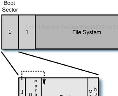
Sector 0 on a floppy disk is called the boot sector. It contains the “bootstrap” code that is loaded by the BIOS start-up process, once a boot device is chosen. Bootstrapping is a term named after the (impossible) action of “pulling yourself up by your own bootstraps,” which is one of those colorful English expressions hijacked by computer people for their own use. Resources available at boot time are limited, and at each stage of the boot process, the capabilities of the system's software increase, until finally the operating system is running, having pulled itself up “from nothing” but a small piece of executable code in the disk's boot sector.
The format of a floppy, then, may be thought of as the boot sector and “everything else,” with the boot sector providing
A jump to boot loader code located in a known place (at the front)
A partition table that contains file system type, disk labels, and so on
The boot loader code
A file system
The format for a floppy disk is shown in Figure 9-1. If you examine Linux commands that create bootable floppies, for example /sbin/mkbootdisk, you will find that they use a command like mkdosfs to create a file allocation table (FAT) file system on the floppy, and then copy other higher level files to the floppy's file system. The mkbootdisk command is really a shell script, so you can examine it for details.
Although it was very common for every system to have a floppy diskette drive in the past, modern systems like laptops and servers are omitting the built-in floppy drive in favor of external USB floppy drives. A 1.4-MB floppy is just not as useful as it once was. We can still fit a Linux kernel onto a floppy, and this is done in the case of the boot disks you are prompted to make during installation.
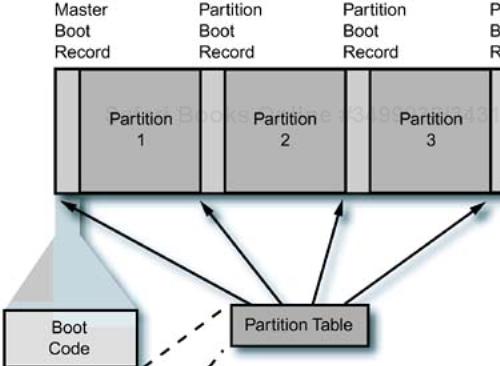
Now we can extend the concepts from the floppy format to the format used for hard disks. The BIOS allows four “primary” partitions on a hard disk—period. There is a “master boot record” or MBR at the start of the disk, and each partition has its own boot record. It looks a little like four large floppies concatenated together, with a few differences. This layout is shown in Figure 9-2.
Because things in the compute world grow incrementally and need to maintain backward compatibility, it is not surprising to see a similar theme played over and over again. Linux assigns device names to the disk configurations, using naming conventions that depend on the type of disk. An IDE uses the device file /dev/hda for the whole disk device, /dev/hda1 for the first partition, /dev/hda2 for the second, and so on, up through the device named /dev/hda4 for the last primary partition on the first IDE disk. This layout is shown in Figure 9-3.
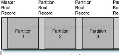
Even though the partitions are shown roughly the same size in the diagram, there is no requirement to make them any particular size. There may be unallocated space on the disk, and any number of primary partitions between one and the maximum of four. One of the partitions is marked as the “active” partition to show that it is the default-bootable partition.
The BIOS scans the system for disks devices and creates numerical descriptors for them. The operating system is then able to query the BIOS to locate which devices are present and to determine how they are partitioned by reading the partition table from the disk's MBR. You can see the information for a Linux system with a dual-channel IDE controller (channels 0 and 1) on the console during the boot process, from /var/log/messages, or by using the dmesg command:
ide: Assuming 33MHz system bus speed for PIO modes; override with idebus=xx
ICH: IDE controller at PCI slot 00:1f.1
ICH: chipset revision 2
ICH: not 100% native mode: will probe irqs later
ide0: BM-DMA at 0x1800-0x1807, BIOS settings: hda:DMA, hdb:pio
ide1: BM-DMA at 0x1808-0x180f, BIOS settings: hdc:DMA, hdd:pio
hda: WDC WD800JB-00FMA0, ATA DISK drive
blk: queue c040cfc0, I/O limit 4095Mb (mask 0xffffffff)
hdc: WDC WD800JB-00FMA0, ATA DISK drive
hdd: LG CD-RW CED-8083B, ATAPI CD/DVD-ROM drive
blk: queue c040d41c, I/O limit 4095Mb (mask 0xffffffff)
ide0 at 0x1f0-0x1f7,0x3f6 on irq 14
ide1 at 0x170-0x177,0x376 on irq 15
hda: attached ide-disk driver.
hda: host protected area => 1
hda: 156301488 sectors (80026 MB) w/8192KiB Cache, CHS=10337/240/63, UDMA(66)
hdc: attached ide-disk driver.
hdc: host protected area => 1
hdc: 156301488 sectors (80026 MB) w/8192KiB Cache, CHS=155061/16/63, UDMA(33)
Partition check:
 hda: hda1 hda2 hda3
 hdc: hdc1 hdc2 hdc3
The first IDE device found is hda, the next IDE device is hdb, followed by hdc, and so forth. SCSI disks follow a similar naming convention, starting with sda, sdb, and so on. People tend to use the device name Xda and the device file, name, /dev/Xda, interchangeably. Let's switch to just the device name from now on, unless we need to specify the device file explicitly for some reason.
In the previous example, the IDE slave device on channel 0 is not used, so it does not show up during the device scan. The second channel, channel 1, has a disk as the master device (hdc), and the slave device is a CD-ROM (hdd). The bus and device scanning order determines which devices are located and the assigned device file name is. (This is very important to know. Adding devices to the system can change the configuration of the device names. For example, USB devices like disks actually show up as SCSI devices [as do some IEEE 1394 disk devices]. If the device is plugged in and the system rebooted, the device file names may be reordered.)
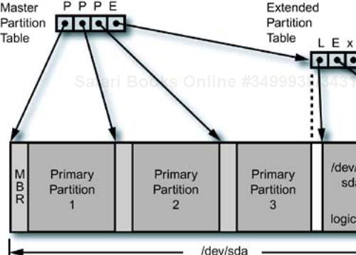
The next step in the partitioning progression is the addition of “extended” disk partitions, which allow a primary partition to be divided into subpartitions, called logical partitions. As you might imagine, four primary partitions may not be enough physical divisions of the disk for some situations, so the extended partition scheme was added to cope with larger disks and more complex system disk configurations.
An example of an extended partition and the associated SCSI device names is shown in Figure 9-4. The partition table in the MBR only has enough space for four physical partition entries, which allows three primary and one extended partition. The partition table in an extended partition contains one logical partition entry, a pointer to the next extended partition, and two empty entries. This creates a linked list of partition table entries.
Note that the boot records in the logical partitions are not accessible as part of the device; they “belong” to an extended partition. For example, if we wanted to save a copy of the MBR, we could simply execute
# dd if=/dev/sda1 of=/tmp/mbr.save bs=512 count=1
This command accesses the first sector (512-byte block) on the device /dev/sda1 and copies it to a file. We could not do this for a logical partition and get what we would expect. If all this seems at once complicated and limiting, you are absolutely correct. The current way things are done depends on history and backward-compatible changes made at every step from MS-DOS (PC-DOS if you remember) to the present. It is entirely possible to create a partition table that confuses both humans and operating systems.
In addition to the “normal” Linux partitions, an Itanium (IA-64) system adds another requirement: the extensible firmware interface (EFI) partition. The EFI environment provides the initial interaction between the hardware boot process and the hardware drivers and operating system that are loaded as the boot process continues. The “stable” storage for EFI is a disk partition, called the EFI system partition, that contains EFI applications and drivers.
Much of what used to be contained in the hardware and interface card BIOSs is now kept in “external” files located in the EFI partition. A standardized loading and initialization process is built into the system's NVRAM, but information that would previously have required flashing the BIOS is loaded from files by EFI at boot time. Updating the files in the EFI partition reduces (but does not eliminate) the need to update the system's firmware.
The EFI partition is a modified FAT file system, and therefore suffers from the DOS 8.3 file name format. This is the familiar DOS eight-character file name and three character file extension convention. If you look into the EFI partition on a Linux system, you will see a file, named elilo.efi, that is responsible for loading the IA-64 Linux kernel into memory and starting it. If there are other operating systems resident on the machine, other boot files will also be visible. They all will have short (or truncated) file names.
The elilo.efi file is loaded and executed by the EFI boot loader, which can also execute other EFI applications, including diagnostics, editors, shells, and network boot managers. There is a simple menu interface to the EFI boot loader that enables selection of the appropriate EFI application at boot time. The exact behavior of your EFI environment depends on the manufacturer of your hardware, so I will not go into any more detail here. Once Linux is started, its behavior is familiar, no matter what the underlying processor architecture.
The addition of the EFI partition to the list of required Linux partitions pushes the absolute minimum (EFI, “/,” and swap) partition configuration to four. This virtually ensures that you will need to place additional partitions into extended partitions. Fortunately, the installation tool allows specifying the partition type (“force to be primary”) or selects the best default configuration based on your partition choices.
The initial boot code for the system “lives” in the MBR and is loaded by the BIOS when the boot device is selected. Once activated, the boot loader has control of what happens next. There are several boot loaders that work with Intel IA-32 Linux, including the Linux loader, lilo, and the GNU grand unified boot loader, grub. For Itanium systems the boot loader is a combination of the EFI menu and elilo.efi.
lilo is a fairly simple-minded boot loader that stores information about the location of the Linux boot files inside the MBR with its boot loader code. This means that every time you make changes to the kernel or initial RAM disk configuration, you must rerun lilo to update the MBR information, or risk having an unbootable system. lilo is sometimes difficult to remove; it likes its home in the MBR and leaves only with great reluctance. (It is a good idea to save the original state of the MBR, if possible, before making changes to it.)
The default boot loader for Red Hat Linux and derivatives is now grub, although lilo is available for hardware situations that require it. I much prefer grub, for one thing, because it is possible to build an independent grub recovery disk that you can use to repair MBR problems and boot the system from a floppy if something goes wrong. All of this is possible with lilo, but it seems to be easier with grub.
Using grub has the added advantage that it can recover from errors and mistakes much more easily. As its name implies, it was designed to be flexible and to provide a unified way of booting multiple processor architectures and disk configurations. Most of the information on grub may be found by executing
# info grub
Using the info command is an acquired skill set, but there is a lot of Linux documentation for GNU tools that is only available in that facility.
The configuration information for grub is kept in /boot/grub, and includes a configuration file, boot loader stages, and file system-specific drivers. The /boot/grub/grub.conf file contains configuration information that is selectable by the user at boot time:
default=0
timeout=10
splashimage=(hd0,0)/grub/splash.xpm.gz
title Red Hat Linux (2.4.20-28.8)
      root (hd0,0)
      kernel /vmlinuz-2.4.20-28.8 ro root=LABEL=/
      initrd /initrd-2.4.20-28.8.img
title Red Hat Linux (2.4.20-27.8)
      root (hd0,0)
      kernel /vmlinuz-2.4.20-27.8 ro root=LABEL=/
      initrd /initrd-2.4.20-27.8.img
Each possible boot option is presented in a menu, with the first entry in the file, the 0 entry, being the default boot selection in this example. Entry 0 is the first entry at the top of the list. The splash image displayed behind the menu is a compressed X Windows pix map (XPM) file, located in the /boot/grub directory. Because /boot may be a separate partition, all file names are relative to the partition, which is (hd0,0), or the first partition on the disk.
Notice that the device names used by grub are different from the device names used by Linux. The specification is for a hard disk and section number (partition) on that hard disk. There is a map file in /boot/grub/device.map, that contains the grub to Linux device mappings for bootable devices on the system:
# this device map was generated by anaconda
(fd0)     /dev/fd0
(hd0)     /dev/hda
The information in this file is generated by the Red Hat installation tool, called anaconda.
The information in each labeled boot section contains a definition for the device that contains the system's root directory, plus a kernel and RAM disk definition. The kernel definition line contains several parameters passed to the Linux kernel as it boots. We will examine Linux kernel parameters in an upcoming section.
You can make a stand-alone grub boot disk with the following commands:
# cd /usr/share/grub/redhat-i386
# dd if=stage1 of=/dev/fd0 bs=512 count=1
# dd if=stage2 of=/dev/fd0 bs=512 seek=1
Note that all data on the floppy is destroyed by this process. Once completed, you can boot grub from the floppy and perform useful recovery operations like searching for a bootable partition, selecting a kernel and RAM disk image, and reinstalling grub into the MBR.
We could write a book on just the boot loaders available for Linux. It's silly, but which Linux boot loader is someone's favorite tends to be intensely personal and a source of occasional heated “discussions.” With this in mind, let's will move on to booting the kernel using your favorite boot loader.
Booting the Linux kernel involves distinct phases, and a different level of software “intelligence” is available at each step. The basic steps are
Boot device selection (default or user input)
Boot the operating system loader from the device
Load the kernel and initial RAM disk into RAM
Start the kernel, passing parameters
Complete transition to final target run level
The hardware initialization culminates with the selection of a boot device, either from a menu or from a default value stored in NVRAM. The operating system loader is executed, and it starts the Linux kernel, passing it parameters that affect its initialization behavior. A list of some of the parameters that can be passed to the kernel is located in /usr/share/doc/kernel-doc-<version>/kernel-parameters.txt, if you have the kernel source Red Hat package manager (RPM) package loaded, or from man 7 bootparam. Both information sources have different lists of options.
First, a word about kernel files, of which there are two “flavors”: compressed and uncompressed. The following listing shows the relative sizes of the kernel files on one of my systems:
# cd /boot
# ll vmlinu*-2.4.20-28*
-rw-r--r-- 1 root root 3175854 Dec 18 10:03
           vmlinux-2.4.20-28.8
-rw-r--r-- 1 root root 1122155 Dec 18 10:03
           vmlinuz-2.4.20-28.8
The compressed kernel is roughly 35% of the size of the uncompressed version. This saves space on the disk, but also makes a bootable floppy possible in the right situations (when the kernel and associated files are less than 1.4 MB total). The kernel is decompressed as it is loaded into memory by the boot loader.
The grub example in the previous section shows two options that are passed to the kernel: ro and root=LABEL=/. The first option initially mounts the root device read-only, and the second option specifies that the kernel should look for a file system superblock that contains a label identifying it as “/,” which is the root file system. As we will see, the Linux file systems allow specifying a file system to mount by a label in addition to a device, to avoid problems caused by devices changing their association with device files resulting from “migration” in the scan order.
The initial RAM disk image is a compressed file system image that is loaded into memory, mounted as the root file system by the kernel during initialization, then (usually) replaced by the disk-based root file system. A lot of Linux boot activities involve manipulation of the initial RAM disk (initrd) contents. We examine manipulating the initrd image in the next section.
As with a lot of features on Linux, a little reverse engineering can help you do some interesting things. The initial RAM disk image is created manually by the /sbin/mkinitrd command, which happens to be a script. You can view the script contents to see exactly what is being done to create an initrd. Let's try running the script:
# mkinitrd
usage: mkinitrd [--version] [-v] [-f] [--preload <module>]
[--omit-scsi-modules] [--omit-raid-modules]
[--omit-lvm-modules] [--with=<module>] [--image-version] [
--fstab=<fstab>] [--nocompress] [--builtin=<module>]
[--nopivot] <initrd-image> <kernel-version>
(ex: mkinitrd /boot/initrd-2.2.5-15.img 2.2.5-15)
[root@ns1 tmp]# mkinitrd /tmp/initrd.img 2.4.22-1.2174.nptl
WARNING: using /tmp for temporary files
Okay, so we made an initial RAM disk image, by specifying the file name and the version string of the kernel, but what are we really doing?
The initrd file contains a miniature root file system, including the directory /lib, which contains the dynamically loadable kernel modules necessary to support the root file system. This is why we specify the kernel version string, because mkinitrd uses this to locate the /lib/modules/<version> directory. It then adds the necessary kernel modules into the initrd file system to support booting from devices and file system types that are not built into the kernel.
Notice that the mkinitrd command allows control over what kernel modules are added to the compressed file system image, along with control over how and when the modules are loaded during the kernel initialization process. We are avoiding a “which-comes-first-the-chicken-or-the-egg” issue: How do you boot the root file system if it resides on a device that requires a module in the root file system? The answer is: By using an initrd with the required module in it that is available to the kernel before the root file system is mounted.
Let's take an initrd apart to see what's inside. Let me warn you, I will be doing some things that appear a little magical if you haven't done them before. I promise to explain what is going on if you bear with me.
# gunzip < initrd.img > initrd
# losetup /dev/loop0 /tmp/initrd
# mkdir image_mnt
# mount -o loop /dev/loop0 image_mnt
# ls image_mnt
bin  dev  etc  lib  linuxrc  loopfs  proc  sbin  sysroot
What I just did was unzip the initrd image, associate the file with a “loop-back” device, mount the loop-back device onto a local directory, then look inside the directory. If we look at the output of the mount command
# mount
/dev/loop0 on /tmp/image_mnt type ext2 (rw,loop=/dev/loop1)
you can see that the loop-back device is mounted on the directory, as if it were an actual disk. The loop-back functionality allows us to mount a file as if it were a device, and access the data in it as if it were a file system (which it is in the case of an initrd).
You can see the directory and file structure inside the example initrd, including a file named linuxrc. This file is run by the kernel when it mounts the initrd. The file contains shell commands that are run by nash, which is a very compact command interpreter developed for just this use.
#!/bin/nash
echo "Loading jbd.o module"
insmod /lib/jbd.o
echo "Loading ext3.o module"
insmod /lib/ext3.o
echo Mounting /proc filesystem
mount -t proc /proc /proc
echo Creating block devices
mkdevices /dev
echo Creating root device
mkrootdev /dev/root
echo 0x0100 > /proc/sys/kernel/real-root-dev
echo Mounting root filesystem
mount -o defaults --ro -t ext3 /dev/root /sysroot
pivot_root /sysroot /sysroot/initrd
umount /initrd/proc
Notice that at the end of the script, the root file system (on the disk) is mounted to the /sysroot directory, then a pivot_root is executed, which switches the root directory in use by the kernel to the disk-based file system. Shortly after the root is pivoted to the disk, the kernel starts the init process (the “parent” process of everything on the system, with a process identifier [PID] of 1 and a parent process identifier [PPID] of 0) from the file system and continues the boot process.
Let's clean up the situation with the mounted initrd file from our example:
# umount /tmp/image_mnt
# losetup -d /dev/loop0
The general booting process for the Linux kernel, and the involvement of the initrd file, are important to our development activities within the cluster. The network system installation tools, network boot tools, and other Linux booting facilities (including the standard system boot from disk) all intimately involve the initrd in various forms and configurations.
Now that you know what is in the initrd, let's examine a few of the kernel parameters that can be passed by the boot loader. A partial list of useful kernel parameters is presented in Table 9-1.
Table 9-1. Kernel Parameters
Parameter | Values | Description | Example |
|---|---|---|---|
|
| Sets system root directory |
|
|
| Sets the path to an NFS root directory on an NFS server |
|
|
| Sets the NFS server address to the IP address given |
|
|
|
| |
|
| Sets the location of the initial RAM disk file relative to the boot directory |
|
|
| Sets the size of system RAM to use in megabytes |
|
|
| Enables ( |
|
|
| Sets the size of the |
|
|
| Mounts the root directory in read-only mode |
|
|
| Sets the console output device and [speed,control, parity] value |
|
|
| Sets VGA mode to 80x25, 80x50, or prompts for mode |
|
Of course, these parameters only scratch the surface of what is available. They are some of the more common ones, and we will be seeing more use of them in upcoming chapters. See the file /usr/src/linux-<version>/Documentation/kernel-parameters.txt for a complete list of the documented kernel parameters.
Administrative and infrastructure systems have varying needs when it comes to local file systems (I will cover specific information about cluster file systems and file servers elsewhere in this book). An administrative node that is responsible for performing multiple system installations at once should provide a local file system that can feed data to the network interface as rapidly as possible. An administrative node that is running an essential service and needs to be highly reliable, might trade performance for immunity from disk failure. One of my customers studied the effect of mirroring the system disk on system reliability. They concluded that, in their environment, they could attain 99.99% (“four nines”) of “up” time merely by buying reliable system hardware and mirroring the system disks.
We need to consider two factors when implementing local storage: the local file system type, and the configuration of the underlying disk storage. Although many commodity servers provide hardware RAID controllers (and Linux supports the more common ones), we can also save money by using the Linux software RAID facility, provided we have configured multiple disks into the base hardware system. Linux also provides a large number of possible physical file system types—everything from DOS FAT file systems to the journaled ext3 file system, which is the default on Red Hat Linux. Type man fs for a complete list of the possible (but not necessarily available) file systems.
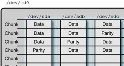
The Linux software RAID facility, also frequently referred to as the multiple device or md facility, provides striping (RAID 0), mirroring (RAID 1), striping with parity device (RAID 4), and striping with distributed parity (RAID 5). Another configuration, linear mode, creates one continuous disk device from multiple disks and provides no redundancy. Each of these behaviors is implemented in a dynamically loaded kernel module.
The md devices on a Linux system are defined in the /etc/raidtab file,[1] and are activated automatically at system boot time, either from the initrd file, if the system disk is on a RAID device, or from the root directory. Although it was a difficult endeavor earlier, most Linux distributions now allow installing the system partitions on RAID devices and include the proper modules in the system initial RAM disk image (initrd) to support this configuration. This means we may gain the extra reliability from mirrored system disks, even if the hardware does not explicitly have RAID capability.
The md device files themselves are located in the /dev directory and are named according to the convention for md devices: /dev/md0, /dev/md1, and so forth. These devices have their configuration and operational behavior specified in the /etc/raidtab file. Once they are initialized, each device has a persistent superblock stored on it that specifies the RAID mode and a UUID (a 128-bit universally unique identifier) for the md device to which it belongs.
It should be noted that the parity calculation is done in software (this is one reason why the facility is called software RAID), and so relies on the speed of the CPU. The system determines the best available parity calculation method at boot time. The following real-life example of an /etc/raidtab file contains the configuration for a RAID 5 array:
raiddev                         /dev/md1
        raid-level              5
        nr-raid-disks           4
        nr-spare-disks          0
        chunk-size              64
        parity-algorithm        left-symmetric
        device                  /dev/sda
        raid-disk               0
        device                  /dev/sdb
        raid-disk               1
        device                  /dev/sdc
        raid-disk               2
        device                  /dev/sdd
        raid-disk               3
This example RAID 5 device has four SCSI disks that are combined into a single md device. The disks that make up the RAID device are divided into 64-KB chunks. This particular RAID device does not have a spare disk, although this is possible. If a disk fails, the array will operate in degraded mode until the disk can be replaced. On repair, the data on the failed disk will be rebuilt from the parity information on the other disk drives. An example RAID 5 configuration is shown in Figure 9-5.
The /proc/mdstat file contains the current status of all active md devices on the system. The /proc/mdstat contents for the example RAID 5 array in the raidtab example is as follows:
# cat /proc/mdstat
Personalities : [raid5]
read_ahead 1024 sectors
md1 : active raid5 sdd[3] sdc[2] sdb[1] sda[0]
      215061888 blocks level 5, 64k chunk, algorithm 2 [4/4]
       [UUUU]
The [UUUU] field represents each of the four disks in the array. If any of the disks are currently rebuilding, the U for that disk becomes a “_” character. The rebuilding process operates within a minimum and maximum I/O rate in kilobytes per second. These current values for these limits are available in the /proc/sys/dev/raid directory, in the files, speed_limit_min and speed_limit_max.
Creating the md device from scratch involves
The system will automatically detect the RAID array and restart it at system boot time. The RAID 5 configuration is useful for bulk data storage when immunity to disk failure is required. Because of the processing required for parity calculation, however, the performance is not optimum for writes. Aside from the parity calculation overhead, in general a RAID 5 array must wait for the parity information to be calculated and written before a given I/O transaction is complete, which has the effect of serializing the I/O to multiple disks. Hardware arrays have cache memory that helps to hide this latency from the host operating system.
The contents of the linuxrc file in this system's initrd is
#!/bin/nash
echo "Loading scsi_mod module"
insmod /lib/scsi_mod.o
echo "Loading sd_mod module"
insmod /lib/sd_mod.o
echo "Loading aic7xxx module"
insmod /lib/aic7xxx.o
echo "Loading xor module"
insmod /lib/xor.o
echo "Loading raid5 module"
insmod /lib/raid5.o
echo "Loading jbd module"
insmod /lib/jbd.o
echo "Loading ext3 module"
insmod /lib/ext3.o
echo Mounting /proc filesystem
mount -t proc /proc /proc
raidautorun /dev/md0
echo Creating block devices
mkdevices /dev
echo Creating root device
mkrootdev /dev/root
echo 0x0100 > /proc/sys/kernel/real-root-dev
echo Mounting root filesystem
mount -o defaults --ro -t ext3 /dev/root /sysroot
pivot_root /sysroot /sysroot/initrd
umount /initrd/proc
Notice that there are more modules to be loaded in this example, because the disk devices are SCSI, and modules for the SCSI interface, SCSI personality, and SCSI general disks are loaded, along with the modules for the RAID 5 devices. The RAID 5 personality module requires the parity calculation module. These modules are loaded and configured in the initrd even though the system's root file system is not located on the RAID 5 device. Why?
The answer to this lies in the fact that the kernel has been upgraded by loading a kernel RPM package on this particular system. Part of the installation process for the kernel RPM module is to generate a new initrd file by looking at the currently active kernel modules. The default behavior is to include disk-related modules in the initrd, regardless of whether they are directly associated with the root disk. The options to mkinitrd can control this behavior if it causes concern or issues, which it doesn't appear to in this case.
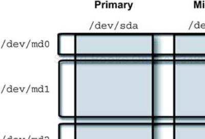
An example of a RAID 1 (mirrored) configuration is shown in Figure 9-6. The Red Hat installation tool, anaconda, allows configuration of RAID 1 devices through the manual disk-partitioning tool: disk druid. This means that you may configure the RAID 1 devices and install the operating system as part of the initial system installation process.
If you haven't configured RAID 1 devices as the system disk before, it is not as straight-forward as it might be. Not that the process is difficult, but determining the correct sequence to keep the partitioning tool happy is potentially frustrating. If you do things in the wrong sequence, the order of your partitions gets “rearranged” for you for no apparent reason. The correct sequence is the following.
Locate the hardware disk devices that you want to use for RAID 1 (
/dev/sdaand/dev/sdbfor SCSI,/dev/hdaand/dev/hdbfor IDE disks). There may be more than one mirror in the RAID 1 set, but this example uses one primary and one mirror.Create a software RAID partition on the first drive (deselect the other potential drives from the list) for
/boot, around 100 MB.Create another software RAID partition on the second drive (deselect the first drive as a potential device from the list) that is the same size as the first (check the displayed size).
Now create a RAID 1 device using the two software RAID partitions. This will become
/dev/md0.Use the same steps to create (at least) the remaining two required RAID 1 devices for the required Linux partitions The minimal configuration requires two partitions: “/” and swap. There are other recommended configurations, such as creating a
/bootpartition, and a separate/varpartition to keep log files from filling the root file system. Your choices will depend on your situation.
Once the partitioning and RAID creation operations are completed, the system installation will follow its normal course. When the system is booted, you can examine the current disk partition configuration to see your handiwork:
# fdisk -l /dev/hda

Disk /dev/hda: 80.0 GB, 80026361856 bytes
240 heads, 63 sectors/track, 10337 cylinders
Units = cylinders of 15120 * 512 = 7741440 bytes

   Device Boot    Start       End    Blocks   Id  System
/dev/hda1   *         1        14    105808+  fd  Linux raid
autodetect
/dev/hda2            15     10268  77520240   fd  Linux raid
autodetect
/dev/hda3         10269     10337    521640   fd  Linux raid
autodetect
Besides the fdisk command, you can also examine (or change, or completely destroy it— always exercise great caution when using partitioning tools like these!) the partition information with parted:
# parted /dev/hda print
Disk geometry for /dev/hda: 0.000-76319.085 megabytes
Disk label type: msdos
Minor    Start       End     Type      Filesystem  Flags
1          0.031    103.359  primary   ext3        boot, raid
2        103.359  75806.718  primary   ext3        raid
3      75806.719  76316.132  primary   linux-swap  raid
Information: Don't forget to update /etc/fstab, if necessary.
Notice the difference in information format between the two commands. Which tool you use is a matter of personal preference, but to avoid confusion it is a good idea to be consistent. Here is an example /proc/mdstat file for a system with RAID 1 system partitions (we will use this particular layout in several examples):
# cat /proc/mdstat
Personalities : [raid1]
read_ahead 1024 sectors
md2 : active raid1 hda3[0] hdc3[1]
      521024 blocks [2/2] [UU]
md1 : active raid1 hda2[0] hdc2[1]
      77517632 blocks [2/2] [UU]
md0 : active raid1 hda1[0] hdc1[1]
      105216 blocks [2/2] [UU]
unused devices: <none>
The last md device in the listing, /dev/md0, is the partition used for the /boot file system. On an Itanium system, the first partition would be the EFI system partition, which should be mirrored like all other partitions. Next in the listing comes the partition used by the root file system, and then finally the swap partition.
The swap partition needs to be mirrored, just like any other essential system partition. In the event of a disk failure, if there is space in use in the failed swap partition, you want the operating system to be able to find the same data in the failed swap partition's mirror. If the swap partition data is not mirrored, this will cause kernel panics. This, of course, invalidates the whole use for mirroring the system disks in the first place: to avoid crashes resulting from disk failures. The /etc/raidtab for this configuration is
raiddev      /dev/md1
raid-level               1
nr-raid-disks            2
persistent-superblock    1
nr-spare-disks           0
    device               /dev/hda2
    raid-disk            0
    device               /dev/hdc2
    raid-disk            1
raiddev                  /dev/md0
raid-level               1
nr-raid-disks            2
persistent-superblock    1
nr-spare-disks           0
    device               /dev/hda1
    raid-disk            0
    device               /dev/hdc1
    raid-disk            1
raiddev                  /dev/md2
raid-level               1
nr-raid-disks            2
persistent-superblock    1
nr-spare-disks           0
    device               /dev/hda3
    raid-disk            0
    device               /dev/hdc3
    raid-disk            1
I have omitted the chunksize definitions that get put into the file by the configuration process. The RAID 1 personality module complains about not needing that information. Looking into the linuxrc file in the initrd for this system, we see
#!/bin/nash
echo "Loading raid1.o module"
insmod /lib/raid1.o
echo "Loading jbd.o module"
insmod /lib/jbd.o
echo "Loading ext3.o module"
insmod /lib/ext3.o
echo Mounting /proc filesystem
mount -t proc /proc /proc
raidautorun /dev/md0
raidautorun /dev/md1
raidautorun /dev/md2
echo Creating block devices
mkdevices /dev
echo Creating root device
mkrootdev /dev/root
echo 0x0100 > /proc/sys/kernel/real-root-dev
echo Mounting root filesystem
mount -o defaults --ro -t ext3 /dev/root /sysroot
pivot_root /sysroot /sysroot/initrd
umount /initrd/proc
Because the RAID 1 devices have their configuration stored in the superblock on the RAID disk members, the system is able to autodetect their presence and start them. This functionality is built into the nash shell that is run at start-up by the kernel. The proper md device files exist in the /dev directory inside the initrd file, and were created when the initrd was built.
The multipath feature in software RAID is relatively new, and appears to be barely documented. In a situation when a hardware RAID array with dual independent controllers is connected via two SCSI or Fibre-Channel interfaces, there are multiple (two) paths to the same storage inside the array. The array is configured to present one or more logical units (LUNs) from within the array to the system, as if they were individual disks. Each LUN, however, is a RAID (0, 1, 0+1, or 5) grouping of physical disk storage within the array, where the RAID behavior is handled internally by the array's hardware.
With multiple controllers, each RAID LUN may be presented to the system twice: once for the primary controller and once for the secondary controller. If one controller fails, there is an alternate path to the same device through another controller and another host interface card. This eliminates single points of failure in the path to the array hardware and its storage. Software RAID allows you to define a multipath device in /etc/raidtab:
raiddev /dev/md4
raid-level           multipath
nr-raid-disks        1
nr-spare-disks       1
chunk-size           32
device               /dev/sda1
raid-disk            0
device               /dev/sdb1
spare-disk           1
This configuration defines a software RAID device in such a way as to allow fail-over in the event that the primary “disk” device (really a LUN from the array) fails. Figure 9-7 shows a hardware RAID array with two controllers and two Fibre-Channel connections to a host system.
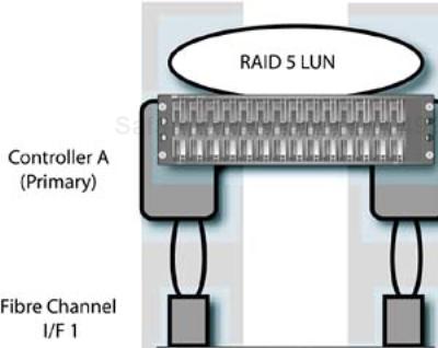
How the single RAID 5 LUN is presented to the system varies, based on the drivers and attachment method (and whether it is a built-in hardware RAID controller), but in this case two SCSI “disk” devices are presented.
The disk devices may be mounted, formatted with a file system (only once, and only with the primary path, please), and treated as if they were actually two separate disks. Both devices, however, point to the same LUN within the hardware array. The level of support and documentation for this feature varies, but is bound to increase as time passes and the functionality matures.
Both the Linux software RAID 5 and RAID 1 configurations can recover from disk failures by activating a spare or switching to a good mirror and allowing you to replace a faulty disk within the software array. If a disk failure is detected in a RAID 1 device, the process of recovery automatically involves copying a RAID 1 disk that is still operational to a spare disk in the RAID set. If the failure is on a RAID 5 device, then recovery automatically recreates the failed RAID 5 disk's data onto a spare using parity information on the operational disks.
In the event that there are no spare disks, the RAID device will continue operating with one less mirror for RAID 1 or in degraded mode (recreating data on the fly) for RAID 5. Without watching for device failures within the software RAID array, a system administrator may not realize that such a failure has occurred. (I will talk about solutions to this further on in the discussion, but the degraded performance may or may not cause user complaints, triggering the necessary investigation, discovery, and repair process.) The RAID driver will regulate the amount of system resources used for a copy or rebuild operation. If no activity is occurring on the system, then the rebuild or copy will proceed at the data rate set by /proc/sys/dev/raid/speed_limit_max per device (the default is 100,000). If activity is present on the system, the activity will proceed at /proc/sys/dev/raid/speed_limit_min (the default is 100).
The raidtools package includes mkraid, lsraid, raidstart, raidstop, raidhotadd, and raidhotremove commands. The mkraid command uses /etc/raidtab to initialize and start the md devices specified to it on the command line. Once the data structures on the md device are initialized, the system can locate and start the RAID arrays without the /etc/raidtab information, as we saw in the previous initrd example in page 185.
The raidhotremove and raidhotadd tools can remove a drive from a software array “slot” and replace it, respectively. This can be used to manipulate spares or failed drives. The basic process to replace a failed drive is to shut down the system, replace the drive, boot the system, and execute raidhotadd /dev/md<N> /dev/<dev>. The software RAID system will begin to rebuild the disk once it is detected. These tools may or may not still be included in your distribution.
Another tool for creating, managing, and monitoring RAID devices is the /sbin/mdadm command, which may partially replace the raidtools on your distribution. The mdadm tool provides similar functionality to some of the raidtools commands, but is a single program that stores its configuration in /etc/mdadm.conf. The mdadm tool does not use the /etc/raidtab information to create the md devices; instead, the device and configuration information is specified on the mdadm command line.
The mdadm command may run in the background as a daemon, monitoring the specified software RAID arrays at set polling intervals (the default interval is 60 seconds). If a failure is detected, mdadm can select a spare disk from a shared pool and automatically rebuild the array for you. The command in general is very flexible, and has Assemble, Build, Create, Manage, Misc, and Monitor or Follow modes. We will look at some examples of its use as we progress, but you should check for its existence (and man page) on your distribution. (You should also go locate a copy of the Software-RAID-HOWTO on http://www.tldp.org/howto. This is a great source of details that I can't include here because of space constraints.)
Most of the Linux partitioning tools allow interactive configuration of partition parameters. It is also possible, however, to feed scripted partition definitions to the tools to recreate complex partitioning schemes automatically with a minimum of typing. Several of the automated system “cloning” or network installation tools use this method to reproduce a disk partition configuration.
One example of a tool that allows flexible partitioning operations is /sbin/sfdisk. The sfdisk tool can list partition sizes, list partitions on a device, check the partition table consistency, or apply commands from stdout to a specified device.
You should not underestimate the power and potential impact of this type of tool. As stated in the man page for sfdisk: “BE EXTREMELY CAREFUL, ONE TYPING MISTAKE AND ALL YOUR DATA IS LOST.” Notice the use of the phrase “is lost”—as opposed to “may be lost.”
As mentioned in a previous section, the partition table for a disk, if it involves extended partitions, will actually be a linked list that is spread across the disk. The sfdisk tool can handle this and will dump the partition information for the specified device:
# sfdisk -l /dev/hda
Disk /dev/hda: 10337 cylinders, 240 heads, 63 sectors/track
Units = cylinders of 7741440 bytes, blocks of 1024 bytes, counting from 0

   Device Boot Start     End   #cyls    #blocks   Id  System
/dev/hda1   *      0+     13      14-    105808+  fd  Linux
       raid autodetect
/dev/hda2         14   10267   10254   77520240   fd  Linux
       raid autodetect
/dev/hda3      10268   10336      69     521640   fd  Linux
       raid autodetect
/dev/hda4          0       -       0          0    0  Empty
This example mirrors (no pun intended) our RAID 1 example configuration. The “+” and “-” characters indicate that a number has been rounded up or down respectively. To avoid this possibility, you can specify that the size is given in sectors and in a format that may be fed back into sfdisk:
# sfdisk -d /dev/hda
# partition table of /dev/hda
unit: sectors
/dev/hda1 : start=       63, size=   211617, Id=fd, bootable
/dev/hda2 : start=   211680, size=155040480, Id=fd
/dev/hda3 : start=155252160, size=  1043280, Id=fd
/dev/hda4 : start=        0, size=        0, Id= 0
In addition to looking at partition information for the existing devices, sfdisk has a built-in list of the possible partition types (numerical labels in hexidecimal) that may be applied to disk partition table entries for Linux and other systems that use the BIOS partitioning scheme. To see that list, use
# sfdisk -T
As you will see, the list is quite long, so I will not reproduce it here. You can manually create quite complex partitioning schemes for multiple operating systems with a little knowledge and a lot of time.
You may be asking, Why would I want to save my partition information? It's on the disk, isn't it? This is a logical question. There are two very logical answers: first to be able to recover from catastrophic failures, and second to be able to use a configuration that works on multiple systems without recreating it by hand. When we begin installing systems with tools like Red Hat's kickstart or the SystemImager tool, reproducing a disk configuration becomes important.
You don't really want to type all the partition information in by hand every time you need it, do you? Having both graphical and text-based tools can be a huge advantage. Being able to use script to recreate disk configurations is extremely powerful and useful.
If you suspect, for some reason, that you have had a disk failure in one of your software RAID arrays, you can use either the lsraid command or the mdadm command to check the status of the raid array. The /proc/mdstat file provides software RAID information on running arrays, but the two software tools provide a lot more options and detailed data, including on devices that may not be part of an active software array. It appears that lsraid is present, even if the raidtools package has been mostly replaced by mdadm on a distribution.
The lsraid command is very useful, because it can also be used to extract a raidtab format output from a functional array. If you are moving things around, or have misplaced the definition for your RAID array, this can be very helpful. An example of extracting the “raidtab” information for our example RAID 5 software array is
# lsraid -R -a /dev/md1
# This raidtab was generated by lsraid version 0.7.0.
# It was created from a query on the following devices:
#     /dev/md1
# md device [dev 9, 1] /dev/md1 queried online
raiddev /dev/md1
      raid-level  5
      nr-raid-disks  4
      nr-spare-disks  0
      persistent-superblock 1
      chunk-size  64
      device  /dev/sda
      raid-disk  0
      device  /dev/sdb
      raid-disk  1
      device  /dev/sdc
      raid-disk  2
      device  /dev/sdd
      raid-disk  3
You can also locate the devices in a RAID array by querying one of the member disks. This will read the superblock information written at the end of the device:
# lsraid -d /dev/sda
[dev 9, 1] /dev/md1 D0E77459.AD65F0FB.7D58622E.74703722 online
[dev 8, 0] /dev/sda D0E77459.AD65F0FB.7D58622E.74703722 good
[dev 8,16] /dev/sdb D0E77459.AD65F0FB.7D58622E.74703722 good
[dev 8,32] /dev/sdc D0E77459.AD65F0FB.7D58622E.74703722 good
[dev 8,48] /dev/sdd D0E77459.AD65F0FB.7D58622E.74703722 good
It is also possible to list failed and good disks and to perform operations on both on-line and off-line devices. Another way to locate information for the arrays is to scan all disk devices that the command can find in the /proc file system. This can also be used to generate the raidtab information:
# lsraid -R -p
# This raidtab was generated by lsraid version 0.7.0.
# It was created from a query on the following devices:
#     /dev/md1 /dev/sda /dev/sdb /dev/sdc
#     /dev/sdd /dev/hda /dev/hda1 /dev/hda2
#     /dev/hda3
# md device [dev 9, 1] /dev/md1 queried online
raiddev /dev/md1
      raid-level  5
      nr-raid-disks  4
      nr-spare-disks  0
      persistent-superblock 1
      chunk-size  64
      device  /dev/sda
      raid-disk  0
      device  /dev/sdb
      raid-disk  1
      device  /dev/sdc
      raid-disk  2
      device  /dev/sdd
      raid-disk  3
If you are fortunate, your Linux version will have both the raidtools and the mdadm command available so that you can make a choice as to which one you will use in a given situation. The raidtools are the traditional way to create and manage software RAID arrays, but there now is another option, the md administration tool (the command previously known as mdctl). The mdadm command can let you know the current operational state of your md device in addition to lots of other nifty operations. Now let's take a look at the capabilities of mdadm.
Remember that creating an array involves initializing the information in the RAID superblocks stored on the devices that are members of the RAID array, including the UUID that uniquely identifies the array. Let's take a look at some of the more common uses for mdadm for similar operations to the raidtools. To create the example RAID 5 array with the mdadm command (and without the information in an /etc/raidtab file), we would use
# mdadm --create /dev/md1 --chunk=64 --level=5
      --parity=leftsymmetric --raid-devices=4
      /dev/sda /dev/sdb /dev/sdc /dev/sdd
The mdadm command is a consistent interface to the software RAID facility, instead of multiple tools, and is well documented. You can list the current status of an md device:
# mdadm --detail /dev/md1
/dev/md1:
        Version : 00.90.00
  Creation Time : Thu May  8 16:48:20 2003
     Raid Level : raid5
     Array Size : 215061888 (205.09 GiB 220.22 GB)
    Device Size : 71687296 (68.36 GiB 73.40 GB)
   Raid Devices : 4
  Total Devices : 4
Preferred Minor : 1
    Persistence : Superblock is persistent
Update Time : Thu Mar  4 00:26:09 2004
          State : dirty, no-errors
 Active Devices : 4
Working Devices : 4
 Failed Devices : 0
  Spare Devices : 0
Layout : left-symmetric
Chunk Size : 64K
Number Major Minor RaidDevice State
0       8    0    0      active sync   /dev/scsi/sdh0-0c0i0l0
1       8   16    1      active sync   /dev/scsi/sdh0-0c0i2l0
2       8   32    2      active sync   /dev/scsi/sdh0-0c0i4l0
3       8   48    3      active sync   /dev/scsi/sdh0-0c0i6l0
UUID : d0e77459:ad65f0fb:7d58622e:74703722
This output shows the UUID that identifies the array members along with the current state and configuration of the array. This is also one source of formatted information, besides /proc/scsi/scsi, from which you can get the full SCSI address information (host, channel, ID, LUN) for each component SCSI device in the array (if your devices are indeed SCSI).
Let's say that a friend handed you a bunch of disks in a box and told you that his system had failed, but he had managed to salvage the still-functional SCSI (or IEEE-1394) disks from a software RAID array on the system. He doesn't remember how he configured the array, and yet he wants to access the devices and retrieve their data. There are several months of work on the array that has not been backed up.
You realize that once you connect the disks to a system, you can use mdadm to query the devices, reverse engineer the array configuration, assemble the array, activate it, and mount it. You power off your system, add the four devices to your SCSI bus, power the system back on, and notice that they are assigned to /dev/sde, /dev/sdf, /dev/sdg, and /dev/sdh by the Linux boot process.
There is a conflict between the definition in the device superblocks (preferred minor number) and an existing md array that prevents the system from autostarting the new array. You perform the following command on the first disk, /dev/sde:
# mdadm --examine /dev/sde

/dev/sde:
          Magic : a92b4efc
        Version : 00.90.00
           UUID : d0e77459:ad65f0fb:7d58622e:74703722
  Creation Time : Thu May  8 16:48:20 2003
     Raid Level : raid5
    Device Size : 71687296 (68.36 GiB 73.40 GB)
   Raid Devices : 5
  Total Devices : 0
Preferred Minor : 1
[... output deleted ...]
Each device is queried in turn, and you suddenly realize that there is one disk missing from a total RAID set of five—and your friend has gone off to a three-martini lunch. You can start the array on an unused md device, /dev/md4, with
# mdadm --assemble /dev/md4 --run
       /dev/sde /dev/sdf /dev/sdg /dev/sdh
This command will assemble the partial array (a RAID 5 array can operate with one disk missing) from only the devices on the command line and attempt to start it. You may also specify information about UUID values or “preferred minor number” (meaning the array was built as /dev/md1) for the devices you want to include.
I hope this contrived example has shown you and your (still invisible) friend the value of using mdadm in performing recovery actions with software RAID devices. To do similar things with the raidtools, you would need to manipulate the /etc/raidtab contents as well as use multiple commands. The recovery would be possible, just not as easy or straightforward.
This example used external disks that were not previously configured on the system that was accessing them. It is possible to specify configuration information about both array component devices and arrays themselves in the /etc/mdadm.conf file for the current system. The mdadm command will search this configuration information to satisfy device lists if you also specify the --scan command-line option.
You can also place UUID or other device or array identification information on the command line to narrow the devices used in the request. For example:
# mdadm --assemble --scan --run
       --uuid=572f9e45:22a34d0f:b6784479:9b2f25d0
This command will scan the device definitions in the /etc/mdadm.conf file and try to build an array out of the devices with UUIDs matching the value specified on the command line.
One last piece of useful functionality from mdadm that we will cover is the ability to monitor and manage software RAID devices automatically. One problem with software RAID devices is that they can have disk members fail, and that fact may not become readily apparent until you look at the proper log file or notice degraded performance. It is more likely that your users will notice before you do.
For basic software RAID array-monitoring activity, when failure information is mailed to root on the local system, we can modify the /etc/mdadm.conf file to add the following lines for our example RAID 5 array:
MAILADDR root
ARRAY /dev/md1 devices=/dev/sda,/dev/sdb,/dev/sdc,/dev/sdd
Next we can enable and start the service:
# chkconfig mdmonitor on
# service mdmonitor start
The monitor mode will report the following events: DeviceDisappeared, RebuildStarted, RebuildNN (percent completed), Fail, FailSpare, SpareActive, NewArray, and MoveSpare. If you read between the lines, you will see that the monitor mode of mdadm is capable of managing spares for a software array. More than that, it can manage a “spare group” that is shared by multiple software RAID arrays.
If a software RAID array with a failed device and no available spares is detected, mdadm will look for another array, belonging to the same “spare group” that has available spare disks. A spare disk will only be moved from an array that has no failed disks. To configure this option, we can add the two ARRAY entries in the /etc/mdadm.conf file and define the same spare group in each entry. The complete format for the configuration file is found in the man page for madm.conf, but a short example is
#PROGRAM /usr/bin/log-madm-events
MAILADDR root
ARRAY /dev/md1 uuid=dae86f86:e8eb4a17:94a5dc17:c232b7c6
      sparegroup=group1
ARRAY /dev/md2 uuid=eaaba077:680d430e:8bb87ddb:c7bac047
      sparegroup=group1
When a spare is moved, an event is generated and is either e-mailed, as in our example, passed to a program that is specified in the configuration file (maybe the logger command to pass the event message to a remote logging server).
Although the program specified in the configuration file for madm might be a preexisting monitor from a system administration package, it might also be a simple script:
#!/bin/sh
# Called with up to three parameters: Event, md device,
# and component device by mdadm when something happens.
#
    EVENT="${1)"
  MDDEVICE="${2)"
REALDEVICE="${3}"
if [ -z "${REALDEVICE}" ]; then
      REALDEVICE="not specified"
fi
/usr/bin/logger -i -p daemon.err -t MDADM --
      "Detected event ${EVENT} on md array
      ${MDDEVICE} component device ${3}."
###
###
For complete information on configuration of the many possible mdadm options for monitoring, see both man mdadm.conf and man madm.
Linux has a wide variety of available file systems, that may be categorized into several general classes. The wide variety of file systems includes many experimental or partially supported versions of file systems that are available on other operating systems. For example, there is an implementation of NT file system (NTFS) from Microsoft Windows, that is available as an experimental (read-only) implementation. The complete list of supported physical file systems may be had by examining the man fs output, but there are many more possibilities beyond that list.
We need to make the distinction between a “physical” file system, which dictates a specific data format on physical disk devices, and a “networked” file system. A networked file system enables remote access to physical storage, usually through some form of network RPC mechanism between clients and the file server. Somewhere in between the physical file system and a networked file system is a “cluster” file system that allows parallel access to physical storage by multiple physical machines.
At least two implementations of popular networked file systems are available on Linux, including the network file system (NFS) originated by Sun Microsystems and the SMB, also known as the CIFS, originated by Microsoft. Cluster file systems, like Lustre, GPFS from IBM, CFS from Oracle, and others, are available as add-on open-source packages or “for-dollars” products. The network and cluster varieties of file systems are covered elsewhere in this book.
Physical file systems may be built into the kernel at compile time or provided as dynamically loaded modules. Even with dynamically loaded modules, however, some modifications to code resident in the kernel may be necessary to support the file system's behavior. These modifications may require special versions of the kernel, or patches, or both. This is an activity that is best left to software experts. Try to find distributions that contain “ready-to-go” versions of these file systems if you need them.
Some of the more common physical file systems for Linux are the ext2, ext3, Reiser, vfat, iso9660 (High Sierra and Rockridge), XFS (from Silicon Graphics Inc.), DOS, and MSDOS file systems. Whew, that's a lot of choices, but variety is the spice of life—so it's said.
Because it is relatively easy to encapsulate the software that implements a file system in a loadable module, it is also relatively easy to load the behavior when you need it, and unload it when you are finished. The “standard” UNIX (and Linux) commands to manipulate file systems, like mkfs and fsck, are front-end interfaces to the file system-specific commands on Linux:
# ls /sbin/mk*fs*
/sbin/mkdosfs /sbin/mkfs /sbin/mkfs.ext2 /sbin/mkfs.jfs
/sbin/mkfs.msdos /sbin/mkfs.vfat /sbin/mke2fs /sbin/mkfs.bfs
/sbin/mkfs.ext3 /sbin/mkfs.minix /sbin/mkfs.reiserfs
/sbin/mkreiserfs
This arrangement provides the same level of flexibility in the available commands as is found in the modules. Use it only when you need it.
Part of what we need to do with the design of our cluster's infrastructure nodes, administrative nodes, and file servers, is choose the proper physical storage device configuration (hardware or software RAID, individual disks, and so forth), build a physical file system configuration “on top of” the storage, and then consider how to use the file system to store and share data efficiently. This section addresses the local aspects of Linux file systems and their use by local processes and the operating system. I defer the potential to “export” them to other clients in the cluster until later.
Another type of file system, the pseudo file system, is also used in the Linux environment, alongside physical and networked file system types. The primary example of this type of file system is the file system hierarchy underneath the /proc directory, which provides access to kernel and driver-related data for the system. The /proc hierarchy is at once “there” and “not there” in terms of a physical existence.
Access to the “files” in this file system actually activates underlying handlers in kernel code that receive, collect, format, and return data to the requestor through the standard file system interfaces (read, write, open, close, and so on). If you were to look for data structures for the /proc file system on a physical disk somewhere, you would have a hard time finding them. If you go back to the file system contents of an example initrd (see page 185), you will see the /proc file system listed and see it being mounted by the linuxrc script. It is an important fixture of even memory-based Linux systems.
Many of the “user space” status-reporting commands that you use daily on the system merely read information from files in /proc, format it, and print it to stdout. The /proc information is central to device debugging, system monitoring, and to tuning the kernel's behavior while it is running. Quite a few of the interfaces in /proc are two way—that is, both readable and writable. We will be using /proc a lot in our activities with Linux.
Another pseudo file system that you may encounter on some Linux distributions (but not Red Hat-derived ones at this point in time) is the device file system, devfs. If you go to the “normal” /dev directory, you will find a lot of files that represent devices, both present and not present, on your system. As a matter of fact, on my system, counting the separate files yields
# cd /dev
# ls -1 | wc -l
   7521
Now, although not all of these are device files, most of them are. I only have, at most, 100 real devices on this system, even counting “invisible” things like PCI bus bridges. Do we really need to create all these files, manage the permissions, and search among them to find the real device when we plug in a USB or Firewire (IEEE-1394) device? With devfs, the answer is a resounding no. What is really being created with the mknod command is an inode that links the device file name and information like major and minor number to a specific device driver or “kernel space” handler that implements its behavior. Strictly speaking, there are no “real” files behind the device files in /dev.
As the kernel discovers devices and initializes their drivers, the driver can register the names of the physical devices it manages under /dev. As dynamic modules are loaded and unloaded in response to new devices, the devices may be registered and unregistered with devfs by the driver. Essentially, what is located in the new pseudo file system hierarchy created under /dev is the current set of available devices, with a reasonable naming convention.
The issue, of course, with changes like this is that of backward compatibility. This is why part of the functionality provided with devfs is the ability to create symbolic links, with the expected names, in the /dev directory. These links point to the appropriate device in the new hierarchy under the /dev directory. The links are created and managed by a daemon, devfsd, that may be configured to create the proper links as part of its behavior.
As an example of the new device names, you might expect the “old”-style disk devices, /dev/hda and /dev/hdb, to be located at /dev/ide/hd/c0b0t0u0 and /dev/ide/hd/c0b0t1u0 respectively. These represent controller 0, bus 0, target 0, unit 0, and controller 0, bus 0, target 1, unit 0. Before you panic (or think, Is he crazy?), these are the device names. There are “convenience names,” which are links created for them /dev/discs/disk0 and /dev/disks/disk1. These links point to directories for the disks that contain disc for the whole disk, and part<N> for the disk's partitions. The old /dev/hda2 would become /dev/discs/disk0/part2 under this scheme.
There is, therefore, a good mapping between being able to use reasonable human names for the devices and being able to find the actual physical hardware devices being used. The devfsd allows multiple schemes for mapping between old names and new names, or for the location of the devfs information (in other words, you can mount it under devfs and use hard links between the old names and the new names). If you want to experiment with devfs in your spare time, you can experiment with installing it. (Its creator, Richard Gooch, has his home page at http://www.atnf.csiro.au/people/rgooch/linux/docs/devfs.html.) It is a great example of a pseudo file system, but I do not delve into it any further here.
The second extended file system for Linux, ext2, replaces the first ext file system, which was an extension of the older Minix file system used under the Minix operating system. The ext3 file system is a journaled version of the ext2 file system.
The ext3 file system is the default file system for Red Hat and derivative distributions. There is still a considerable amount of confusion in some documentation (and commands) between the ext2 and ext3 file system. Just remember that the major difference is the presence (ext3) or absence (ext2) of a journal.
An example of this ext2/ext3 confusion is that you use the mke2fs command to create an ext2 or an ext3 file system. There is no mke3fs command. Likewise, you use e2fsadm to shrink or grow an ext2/ext3 file system within a partition (especially if it is located on a logical volume manager [LVM] partition[2], tune2fs performs performance tuning functions on either file system, and e2label changes the file system label that can be used by mount and /etc/fstab instead of a Linux device name. It's just one of those things. C'est la vie et c'est le Linux.
One of the first things we should do is learn to look at the parameters currently in use by an existing ext file system (from now on, we will be referring to ext3 unless explicitly stated otherwise). We can dump the current file system information:
# dumpe2fs -h -ob /dev/md1
dumpe2fs 1.27 (8-Mar-2002)
Filesystem volume name:   BIGDATA
Last mounted on:          <not available>
Filesystem UUID:          2f191424-ffb8-4449-a6ad-6045606bff71
Filesystem magic number:  0xEF53
Filesystem revision #:    1 (dynamic)
Filesystem features:      has_journal needs_recovery sparse_super large_file
Filesystem state:         clean
Errors behavior:          Continue
Filesystem OS type:       Linux
Inode count:              210048
Block count:              53765472
Reserved block count:     2688273
Free blocks:              24026463
Free inodes:              174825
First block:              0
Block size:               4096
Fragment size:            4096
Blocks per group:         32768
Fragments per group:      32768
Inodes per group:         128
Inode blocks per group:   4
Last mount time:          Thu Mar  4 00:26:10 2004
Last write time:          Thu Mar  4 00:26:10 2004
Mount count:              3
Maximum mount count:      23
Last checked:             Sun Feb  1 10:23:53 2004
Check interval:           15552000 (6 months)
Next check after:         Fri Jul 30 11:23:53 2004
Reserved blocks uid:      0 (user root)
Reserved blocks gid:      0 (group root)
First inode:              11
Inode size:    128
Journal UUID:             <none>
Journal inode:            8
Journal device:           0x0000
First orphan inode:       0
This is the information kept in the file system superblock, which normally is cached in memory if the file system is mounted (it can fall out of the cache). Notice the following from the information:
The file system has a volume name (label) associated with it:
BIGDATA.The file system is described by a UUID like some other objects we have encountered in Linux.
We see that the file system has a journal (it is therefore
ext3), needs recovery (has been written to), and has attributes associated with it calledsparse_superandlarge_file.There is information listed about the current free inode count and other disk data structures.
The block and fragment sizes are both 4,096 bytes (4 KB).
Information is listed about the mount times and the next file system check to be performed.
Finally, we see listings for journal information, such as the inode and the journal device (which can be an external disk device).
Discussing some of these points will lead us to some salient features of the Linux ext file systems and their operating parameters.
As was mentioned in an earlier section, the Linux device file assignment scheme can result in physical devices migrating from one device file to another, say from /dev/sda to /dev/sdb, if a new device is discovered ahead of it in the chain. This spells disaster if the device contains essential system partitions, like the root file system. Let's look at /etc/fstab for guidance in the file system mounting parameters:
# cat /etc/fstab
LABEL=/         /        ext3   defaults   1 1
LABEL=/boot     /boot    ext3   defaults   1 2
LABEL=BIGDATA   /bigdata ext3   defaults   1 3
Notice that instead of a device like /dev/hda or /dev/md1 in the first field, there is a label definition. The system will scan the superblocks on all disks to find labeled file systems to which to apply the mount commands. This can make the system immune to “device migration” issues.
The file system labels are created in the superblock with the e2label command. To change the label from BIGDATA to DATABASE, we would execute
# e2label /dev/md0 DATABASE
The label field can be at most 16 characters, or it will be truncated. The label may also be set with
# tune2fs -L DATABASE /dev/md0
and at the time of the file system's creation by the mke2fs command.
The command that would create the example file system and set most of the parameters that are visible in the superblock is
# mke2fs -b 4096
                    -j -J size=400
                    -L BIGDATA
                    -O sparse_super
                    -T largefile
/dev/md1
This command sets the block size to the maximum 4 KB, creates a journal that is 400 MB in size (the maximum), sets the volume label to BIGDATA, creates the file system with fewer superblock backup copies to save space, and sets the inode-to-file ratio to one inode per 1 MB of file system space.
The file system block size is very important to overall performance. For fast I/O channels and disks, the system must be able to move enough data per I/O request to keep the channel and the disk busy transferring data, or performance will suffer. The 4 KB maximum block size for ext file systems appears to be tied more to the Intel IA-32 physical page size in memory, rather than the need for performance. Other UNIX systems allow file system blocks and transfers up to 64 KB at a time, which can keep the hardware busier transferring data. I keep hoping for larger block sizes with ext file systems, but for now we have to go to other file systems, like XFS (not to be confused with the X Windows font server: xfs), to get bigger file system blocks.
I defer the journal parameter discussion until the next section. The file system label is being set at creation time in our example, along with two other options that affect the quantity of superblock and inode data structures on the disk. Those options are sparse_super and largefile.
The sparse_super option affects how many copies of the superblock are spread over the file system. Copies of the superblock are kept in known locations, based on the block size of the file system. The first copy is found at block 8193 (1-KB file system blocks), block 16384 (2-KB file system blocks), and block 32768 (4-KB file system blocks). The alternate superblock may be specified to e2fsck if the primary is corrupted for some reason (like an aberrant dd command to the wrong location on the wrong device). The location of the superblock copies is printed when the file system is created with mke2fs, if the -n option is specified.
Specifying largefile uses a precalculated inode-to-file data ratio of one inode per 1 MB of file data. The largefile4 value specifies one inode to 4 MB of data. Using news creates one inode for every 4 KB of file data. Care must be exercised to create enough inodes, otherwise the file system will report “full,” with what appears to be plenty of data space remaining. Which value is correct depends on the type of data stored in the file system. On the other hand, creating too many inodes will waste file system space that could be used for data storage rather than meta-data.
The size of the disk-based journal is important, especially if you are using the file system for heavy I/O traffic on systems like a file server. If the journal fills with data being updated to the file system, the I/O to the file system will stop until the journal is emptied. How you mount the file system will determine how the journal is used. There is a kernel process, called kjournald, that is responsible for “playing the journal” to the file system. You can watch its behavior with performance tools like top to see what is happening.
There are three options for the journal behavior that may be set in the /etc/fstab file entry for mounting the file system, in place of the defaults token. You can check the man page for the mount command to see all the file system-specific mount options for Linux file systems, including ext3. A lot of behavior may be determined by the mount options for the file systems.
Before I discuss the ext3 journal options, we need to differentiate between two types of data that are written to the file system: file block data and meta-data. The file block data is pretty straightforward: It is the actual data that makes up the user-visible file contents. The meta-data is the information about the file, such as the directory information and the inode data that is not resident inside the file, but still gets written to the file system. Both sets of data must be consistent, or corruption and errors result.
The journal (or on some systems, “log”) exists to ensure that if a program or the operating system is interrupted in the process of updating data in the file system, the actions are being tracked and any mismatch in state between file data and meta-data can be corrected. The level of consistency may be controlled by the journal options at mount time. The ext3 journal options are
data=journal, which writes all data destined for the file system to the journal firstdata=ordered, which forces all file data to the main file system before its meta-data is written to the journaldata=writeback, which can write the file data and meta-data without preserving the order in which it is written
These options specify the behavior for file data; meta-data is always journaled. The default behavior, if none is specified, is data=ordered. You should carefully evaluate the options and their effect on the performance of your systems and the integrity of your data.
To disable journaling and drop back to ext2 file system behavior, you can execute
# tune2fs -O ^has_journal
Other options may be cleared as well, such as sparse_super, but this will force changes to the file system data structures that must be performed by running e2fsck after the operation.
The behavior and performance of a physical file system is tied to the underlying storage geometry on which is written. The ext file systems acknowledge the need to manage stripe sizes on underlying RAID 5 devices by providing an optional value for the “stride” of the underlying RAID array in terms of file system blocks per software RAID chunk. Figure 9-8 shows an example RAID stride configuration.
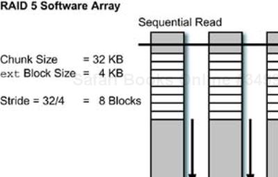
The special RAID behavior is enabled with the -R stride=<N> option to mke2fs at file system creation time. In this case the value to specify for the stride is the number of file system blocks per underlying RAID stripe. If, for example, the underlying RAID array has a 32-KB stripe size and a 4-KB block size, the stride would be set to 32 KB divided by 4 KB, which equals a value of 8 blocks.
Benchmarks with tools like iozone (available from http://www.iozone.org) show that there is an increase in performance based on using this option. How large the performance gain is will depend on factors including the RAID chunk size, physical disk speed, the I/O channel type (SCSI, IDE, and so on), and the system's I/O capabilities. Before settling on a particular configuration, you should run benchmarks to determine the optimum settings for both your RAID devices and the file system. (At the very least you should consult the software RAID HOWTO at The Linux Documentation Project [http://tldp.org/howto/software-raid-howto-5.html] and carefully read the performance information. There are some other underlying data structure alignment issues of which to be aware.)
The defaults token in the /etc/fstab file will cause an ext file system to be mounted with the options listed in Table 9-2. Yet another default that is important to the performance of frequently accessed file systems is the atime option, which causes the inode information to be updated each time the file is accessed. Mounting a file system with noatime specified in the options will disable this behavior and potentially save inode updates to the disk.
Table 9-2. Default Options for the mount Command
Other file system mounting options affect the way that files or directories inherit the group ID on creation. The default behavior, signified by either nogrpid or sysvgroups, causes a file or directory being created to take the group ID (GID) information from the creating process, unless the setgid bit is set on the target directory. In this case, a file being created will take the GID of the parent directory, and a directory being created will also inherit the setgid bit from the parent directory.
The opposite behavior, indicated by either grpid or bsdgroups, will cause a file or directory being created to inherit the GID of the enclosing parent directory. The options, then, may be set file system wide, or controlled on a per-directory basis. The most flexible way to allow the BSD inheritance is to maintain the default (SYSV) inheritance behavior, and use the setgid bit on directories that you wish to have the BSD behavior.
One file system that is useful if your systems have plenty of memory and require the equivalent of a RAM disk is tempfs. This file system, as you might guess, has no protection against data loss in the event of system failure or power loss. It can be used to accelerate operations that create lots of small temporary files.
The possible mount options for the temporary file system are size=<Nbytes>, nr_blocks=<N>, and nr_inodes=<N>. Each of the numerical values may have the suffixes k, m, or g for kilobytes, megabytes, or gigabytes respectively. To create and mount a 100-MB tempfs file system, you can use the following mount command:
# mount -t tempfs -o size=100m /dev/ram /mnt/scratch
There are multiple devices that match the pattern /dev/ram*, so there may be multiple instances of the tempfs active. The default size, by the way, is 50% of RAM, so be careful to specify the real amount you want.
One file system that is readily available on Red Hat and derivative distributions is the Reiser file system. Some of the commands are: mkreiserfs, reiserfsck, resize_reiser, and reiserfstune. I have to admit that I have limited experience with implementing the Reiser file system compared with the ext and XFS file systems. Rather than appear more foolish than I already am, I will leave Reiser for my next book.
The XFS file system proved to be the highest performing file system I tested in one large cluster project. The difficulty with XFS for most situations is that it requires you to patch and rebuild the kernel to add functionality. Although the effort is well worth it, we do not have space to cover the skills needed to patch, rebuild, and test the Linux kernel.
If you are fortunate enough to have a handy kernel programmer, she can do the work in a reasonably short time, so you should not take my avoiding the subject as a negative recommendation, only an attempt at being realistic. In tests that I ran, XFS was 31% faster than ext3 for a six-disk software RAID device built with ultra320 SCSI drives. (I attribute this to in-memory block caches, larger block sizes, and other XFS features. We benchmarked these configurations to death, so please just accept my numbers and don't send fan mail for your favorite file system.)
We do not have space to examine the finer aspects of file system tuning here. It involves lots of single changes to parameters, followed by tedious benchmarking. So, I thought it best to mention several “pointers” that can lead you to some advanced aspects of I/O tuning at the device driver level.
At the individual hard disk level, it is possible to tune the system I/O queue latency to the device driver. At this level, you are working with the I/O “elevator,” which is the Linux I/O scheduler. See the
manpage for theelvtunecommand for more (but sketchy) details.Investigate tagged queuing for the various disk drivers (SCSI) that may be active on your system. For heavy I/O traffic on file servers, it may be beneficial to increase the size of the request queues. Some of this tuning may be done through files in the
/procfile system.It is also possible to tune the drivers that provide the disk interface support. You can get a list of a module's parameters with the
modinfocommand. Start with anlsmodcommand to list the active modules, then usemodinfoto look for tuning opportunities.
Always remember that this level of tuning (very low level) has inherent risks. The driver may not actually work as advertised. Changes you make may damage hardware. You should never perform tuning on a production system without adequate testing. The word adequate is defined differently in different environments.
SMART is an acronym that stands for self-monitoring analysis and reporting technology. This technology is built into late-model SCSI, IDE, and ATA disk drives, and collects information produced internally by the disk hardware and firmware. The software package is capable of being used to report errors, monitor temperature parameters, and examine other useful information. The SMART daemon may also have the drives run self-tests at regular intervals.
The SMART software consists of a daemon and its configuration file /etc/smartd.conf, along with a control program smartctl. The behavior of the software differs from release to release. Red Hat 8.0 had only a bare-bones daemon and the control program, but no configuration file for the daemon. The Fedora Core distributions have better documentation on the components than earlier Red Hat-derived distributions, and appears to support a lot more monitoring functionality and control over the daemon's behavior.
To determine whether your drives are supported, you can run the control program on them, as in this example on an older ATA disk drive on an IDE controller:
# smartctl -a /dev/hda smartctl version 5.21 Copyright (C) 2002-3 Bruce Allen Home page is http://smartmontools.sourceforge.net/ === START OF INFORMATION SECTION === Device Model: IBM-DAQA-33240 Serial Number: 1Y55Y0J4714 Firmware Version: R6ORA52A Device is: Not in smartctl database [for details use: -P showall] ATA Version is: 3 ATA Standard is: ATA-3 X3T10 2008D revision 1 Local Time is: Sun Mar 14 00:17:02 2004 PST SMART is only available in ATA Version 3 Revision 3 or greater. We will try to proceed in spite of this. SMART support is: Ambiguous - ATA IDENTIFY DEVICE words 85-87 don't show if SMART is enabled. A mandatory SMART command failed: exiting. To continue, add one or more '-T permissive'options.
The daemon's ability to communicate with the drive depends on the command language version implemented in the drive itself. We may not be able to enable all the features fully, but let's try to enable SMART monitoring on the disk drive, despite the ambiguity noted in the previous messages:
# smartctl -s on  /dev/hda
smartctl version 5.21 Copyright (C) 2002-3 Bruce Allen
Home page is http://smartmontools.sourceforge.net/
=== START OF ENABLE/DISABLE COMMANDS SECTION ===
SMART Enabled.
Deciding to play it safe, because this system has disks on the borderline of compatibility, I only enabled the minimal checking in the /etc/smartd.conf configuration file. Logging goes to the syslog facility by default, but e-mail can also be added:
# A very silent check. Only report SMART health status if it
# fails. But send an email in this case
/dev/hda -H -m [email protected]
/dev/hdb -H -m [email protected]
/dev/hdc -H -m [email protected]
Starting up the daemon is the next step:
# chkconfig smartd on
# service smartd start
Messages logged in the /var/log/messages file indicate that, even though the disk types are not found in the database of disk models used by the smartd daemon, the disks are being monitored by the daemon:
Mar 14 00:24:29 ns1 smartd[28761]: Device: /dev/hda, is SMART
      capable. Adding to "monitor" list.
Mar 14 00:24:29 ns1 smartd[28761]: Device: /dev/hdb, opened
Mar 14 00:24:29 ns1 smartd[28761]: Device: /dev/hdb, not found
      in smartd database.
Mar 14 00:24:29 ns1 smartd[28761]: Device: /dev/hdb, is SMART
      capable. Adding to "monitor" list.
Mar 14 00:24:29 ns1 smartd[28761]: Device: /dev/hdc, opened
Mar 14 00:24:30 ns1 smartd[28761]: Device: /dev/hdc, not found
      in smartd database.
Mar 14 00:24:30 ns1 smartd[28761]: Device: /dev/hdc, is SMART
      capable. Adding to "monitor" list.
Mar 14 00:24:30 ns1 smartd[28761]: Monitoring 3 ATA and
      0 SCSI devices
Mar 14 00:24:30 ns1 smartd: smartd startup succeeded
Mar 14 00:24:30 ns1 smartd[28763]: smartd has fork()ed into
      background mode. New PID=28763.
The default polling interval for the smartd process to query the drives it monitors is 30 minutes, which may not be suitable for systems that are running compute-intensive jobs that should not be interrupted. Certainly on server systems like infrastructure, administrative, or file server nodes, this monitoring is potentially worth the system overhead. The ability to predict drive failures is certainly something that we should not turn down lightly, especially on systems that are central to the operation of the cluster.
For information on the many configuration options available, see the man pages for smartd, smartd.conf, and smartctl. Also, in case you missed the Web page for the software in the earlier messages, it is located at http://smartmontools.sourceforge.net.
The information contained in this chapter should help you get a good start toward configuring the local file systems on the administrative and infrastructure nodes in your cluster. Much of what we discuss here is also useful in configuring the compute slices (local scratch file systems or system disks), file servers, or any other cluster component that uses Linux software RAID or needs to provide a local file system.
Selecting the proper RAID configuration to protect data or to provide high availability for system disks is one skill that you should take away from reading the details we discuss. There is a lot of flexibility and functionality available not only as part of the standard distributions, but as “external” open-source packages as well. We are very fortunate to have a full tool kit when it comes to file systems and the underlying use of disk resources.
TIP
Software RAID on Linux is an inexpensive way to improve system reliability and data availability for infrastructure systems. For mirroring system disks, use RAID 1; for protecting data availability, use RAID 5. Order your hardware with the required multiple internal disk drives.
We did not cover some obvious disk-related features, like LVM, because there simply is not space to contain all the information on all the possible choices for file system and disk configurations in Linux. Rather than being a disadvantage, however, with a little exploring you will locate more possibilities for your Linux “bag of tricks.” Don't be afraid to explore further.
[1] This is true for devices created and managed with the raidtools commands, like mkraid, but there is now another option on some versions of Linux, the mdadm command which I discuss later.
[2] The original LVM technology was donated to the OSF by IBM, for inclusion in its OSF/1 operating system. Similar functionality is available on HP-UX, Linux, and several other operating systems. If you are familiar with LVM, you will probably be right at home with Linux's version. See man lvm for details and to expand your command repertoire by about 30 to 35 Linux commands.