
SME elicitation is the process by which we alleviate, at least temporarily, SMEs from the effects of their biases so that they can think more clearly and creatively about what the future might hold or what might veil their ability to possess certain knowledge. During the process, we facilitate an enumeration of causative factors that can affect the outcome of an uncertainty that was identified in the influence diagram, and then we assign—via the expert guidance—a measurement to the uncertain outcome as a range of probabilities that spans the range of the outcome.
The Good SME
Unlike the rest of us, SMEs are especially versed in the underlying causes and mechanisms, along with the nuances and fine distinctions, that affect events associated with their area of concern, study, or responsibility. SMEs are not just scientists or industry gurus, although they certainly can be. They are people who possess close at hand familiarity with an idea, a process, a program, or an activity. They could be a lead researcher in your R&D group, or they could be the director of sales, an account manager, or the lead supervisor for a given shift. The consideration for who is an SME is not based so much on their credentials as it is their experience and deep working knowledge.
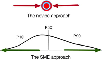
The thinking process of a novice leads to posturing cleverness that results in a much too narrow consideration of outcomes compared with the range of outcomes proposed by an SME
The novice essentially postures a level of precision that admits to requiring a higher quality of information than the current level of uncertainty about a situation reasonably permits. In this sense, they are producing an assumption, a statement about the state of nature in a given context that borders on axiomatic. SMEs, on the other hand, provide assessments; that is, conditional and contingent statements about the possibilities of outcomes that reflect their internal mental disposition that they just don’t know precisely what will occur. SMEs are skeptics.
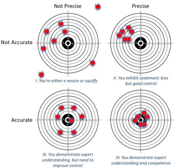
An example of accuracy versus precision
Conduct the Assessment
- 1.
Define the uncertain event.
- 2.
Identify sources of bias.
- 3.
Postulate and document the causes of extrema.
- 4.
Measure the range of events with probabilities.
Define the Uncertain Event
Defining the uncertain event simply means that you will produce a statement that allows you or others to determine, without contention, that an event occurred or that it occurred in a certain way pertinent to the analysis at hand when the facts of the event are examined a posteriori. Determine if the event will occur in discrete values (e.g., [True or False], or [A, B, C]) or along a continuous scale (e.g., costs, revenue, temperature, mass). Explore how the SME thinks about the event and in which units (if any).
The goal is to produce a definition that would pass the so-called clarity test. The clarity test requires that a clairvoyant, who has access to all possible information, be given the definition of the uncertain event. The definition should permit the clairvoyant to make a determination about the event without requiring the clairvoyant to make any special judgments to determine that his or her data satisfies the definition.
Identify the Sources of Bias
Common thinking traps or errors that often plague business people are entitlement bias and wishful thinking. Entitlement bias is related to thinking that just because one has been successful in the past with important business initiatives that future success is not only possible, but virtually certain. This behavior is also related to expert bias , a state of mind in which a person with extensive and often publicly recognized experience in a field of practice regards his or her predictions about future outcomes as incontrovertible. Wishful thinking occurs when people believe that their plans will work as designed simply because they planned them and visualized the outcome (“If we build it, they will come”), or because they have strong emotional investment in the outcome that they desire.
Some of the common cognitive illusions that show up in uncertainty assessments are availability bias and anchoring. Availability bias is the tendency to use recently observed, emotionally impactful, or easily accessible information to lend belief that a certain state of affairs is the case or that an eventual outcome will be the case. Availability bias has a close cousin in confirmation bias (sometimes called “cherry picking”), which is the selective observation of evidence used to justify or buttress preconceived notions or closely held beliefs. To make a playful inversion on the warning commonly printed on rearview mirrors, availability bias drives the perception that images in the mirror are actually closer than they really are. Anchoring is the tendency of the mind to work from the first value that it conceives as a reference point for all other variation around it. Both availability bias and anchoring drive a tendency to believe that initial impressions serve as best guesses for most likely future outcomes.
To begin addressing these biases, ask the SME to describe any recent events or memorable events that come to mind associated with the event in question. Has something related to the event in question appeared in the news? Has there been a recent exposure to the event with a given value associated with the outcome?
If it is not obvious, ask the SME if there is a desirable outcome associated with the event. Would the SME, or those he or she supports, desire a higher or lower outcome or a targeted outcome?
Finally, explore how the outcome might affect the SME personally. Are there preferences, motivations, or incentives that might be associated with the SME and the event? Is the SME compensated in any way for the event occurring at some degree or level of outcome?
This line of questioning should help to reveal confirmation and availability bias, motivational bias, and wishful thinking, among others, at work in the mind of the SME. As a friend of mine says, “Confirmation bias is the root of all evil. And wishful thinking is root fertilizer.” These must be rooted out and exposed.
Postulate and Document Causes of Extrema
Ask the SME to imagine the extreme case representing the opposite direction of the desired outcome. Explore what might have caused this outcome to occur. What had to occur for the future to be in the extreme outcome described? What are those factors? Repeat this process for the opposite extreme. Record the factors for each extreme in separate columns. When you finish tabulating the causative factors, place a quick rank of importance on the top three or four causes on the low and high side. Later, when you go back to consider risk mitigation on the uncertainty, if it’s required, you might want to consider these higher ranked factors first for risk management or risk transfer.
Be sure to emphasize that at this point you are not seeking a number or a value. Resist the tendency to get a value as a starting point because that introduces anchoring. The objective is to counteract anchoring and availability biases by getting the expert away from their preconceived notions or influenced inclinations.
Example of Construction Engineer Acting as SME
Rank | Reasons for Low | Reasons for High | Rank |
|---|---|---|---|
1 | Single source contractor. | Lack of market availability of steel. | 1 |
2 | Good weather permits favorable work conditions. | Inclement weather creates unfavorable work conditions. | 2 |
3 | Working with preferred supplier to use readily available steel shapes. | Multiple bidders. | 3 |
Use of assumed equipment loads for early design. | Coating used: galvanized and epoxy. |
Rationales for Outcomes
Reasons for Bid Loss | Reasons for Bid Win |
|---|---|
• We do not have good customer intimacy at multiple levels in the customer organization and have not directly vetted our solution with them. | • Our management and technical approach address the customer’s needs and has been indirectly vetted (e.g., via Q&A, through consultants, industry briefs/interchanges, through team members) with the customer. Initial feedback seems positive. |
• We have limited relationships with the customer and depend on open sources, public forums, and meetings to get information about their budget, underlying problems, tendencies, and needs. | • We have sufficient time to show the customer key elements of our solution and obtain direct feedback. |
• We understand some of the parameters of the opportunity but knowledge gaps cause some uncertainty in our offer or competitive position. | • We have most of the facilities required to execute this program. What is left to fully execute, we can obtain later as it will not be needed in the early stages. |
• We are missing an experienced and qualified program manager, technical leads, or appropriate SMEs, so we must rely on subcontractors to fill these positions . | • We will price this to win the business, even if it means a razor-thin margin, because it will provide an entry point for future business. |
• A single award is expected, and there are multiple bidders. The odds are against us just by the number of bidders. | • We know the competitor’s approach and have one that is significantly better with customer recognized discriminators. |
• We have experience with similar programs; however, added effort is needed to clearly demonstrate relevance to receive good customer ratings on the bid. | |
• We only have a rough idea of the customer’s budget based on open source information. | |
• This is new capability for a new customer. They might not have the full competency to assess the best offered solution. |
Measure the Range of Uncertain Events with Probabilities
Before proceeding with quantifying the uncertain event with the SME, assure the SME that the purpose of the interview is not to acquire a commitment or a firm projection about the outcome. You are merely trying to measure the overall uncertainty you face with the event. You should also assure the SME that you are not asking the SME to know the probabilities you are trying to assess as if probabilities are a thing or an intrinsic property of an event. Rather, you want to determine, by comparison to a defined lottery or game, the odds at which the SME is indifferent to choosing to play the lottery to win a prize or calling the outcome of the event in question to win a prize. The point of indifference for them is their subjective degree of belief—the probability—that the event will occur as defined.
There are generally two kinds of uncertain events that an SME will be called on to assess: discrete binary events and continuous events.
Discrete binary events are those that produce either a TRUE or FALSE state to describe the outcome of the event, that it either occurred or did not. Examples of this kind of event could be “win the deal,” or “Phase 1 succeeds,” or “Plaintiff claim is dismissed.” The SME will assess the probability of one of the states. The probability of the complementary state must be 1 - Pr(state) by definition of the laws of probability. Under no circumstances can an SME assess the probability of one state, say TRUE, to be Pr(TRUE) = 0.25, and then assert that Pr(FALSE) = 0.55 or Pr(FALSE) = 0.95 without revealing a mental incoherence about the definition of the event. If this does occur, explore what is missing from the definition that might have led the SME to such incoherence.
Continuous events are assessed across an effectively infinitely divisible range with several probabilities, often at the 10th, 50th, and 90th percentile intervals. Examples of these kinds of events might be “capital cost of the reactor,” or “duration of activity 25,” or “sales in quarter 1.” The p10 value is the value of the event at the 10th percentile for which the SME believes there is yet a 1/10 chance that the event outcome could still be lower. Conversely, the p90 value is the value of the event at the 90th percentile for which the SME believes there is yet a 1/10 chance that the event outcome could still be higher. The p50 value (or the median) is the value at which the SME considers that the outcome faces even odds or a 1/2 chance that the outcome could be either higher or lower.
Discrete Binary Uncertainties
Tell the SME he or she will have the hypothetical opportunity to win a prize by opting to play one of two games: Either the SME correctly calls the event occurring, or he or she can play a lottery by pulling a blue token from an urn or spinning an arrow on a wheel of fortune such that it lands on a blue sector for success. The choice to accept either the lottery or to call the outcome of the event is based on the odds presented for the lottery. If the SME thinks the odds of winning the lottery exceed the perceived odds of correctly calling the outcome of the uncertain event, then he or she should play the lottery. On the other hand, if the odds of winning the lottery are lower than the perceived odds of calling the event, then the SME should call the event. After a choice is made, the odds on the lottery are updated such that it should be more difficult to make a clear choice. This process is repeated until the SME is indifferent to choosing either game to win the prize.
- 1.
In the first iteration, produce a random number between 0 and 1, but never 0 or 1. Let Pr_1 be the initial probability of winning the lottery.
- 2.
If the SME prefers the lottery, the lottery probability is too high. Update the next probability to half of the previous probability: Pr_2 = Pr_1 / 2.
- 3.
If the SME prefers calling the event, the lottery probability is too low: Pr_2 = (1 + Pr_1) / 2.
- 4.
If the SME starts with the lottery and continues to choose the lottery, then Pr_i+1 = Pr_i / 2. If the SME starts with calling the outcome and continues to call the outcome, then Pr_i+1 = (1 + Pr_i) /2. However, as soon as the SME switches the game to pull back on overshoot in the last iteration, the probability updates as Pr_i+1 = (Pr_i* + Pr_i) / 2, where Pr_i* is the last highest probability before the SME switches from playing the lottery to calling the outcome, or Pr_i* is the last lowest probability before the SME switches from calling the outcome to playing the lottery. In this way, the bracket of probabilities narrows and converges on a value where the SME should be indifferent to switching again.
- 5.
Repeat Step 4 until the SME is indifferent to choosing either game to win a prize.
The following steps demonstrate the session with the previously described sales manager who assessed the discrete binary probability of winning a competitive bid for a government contract. Each step is illustrated by a result from this online tool 1 to facilitate the visualization of lottery probabilities on each iteration as the SME converges on an indifference point. Recall that the bid team initially expressed a high degree of confidence that their company would win the bid. After going through the rationale eliciting process, however, they realized that there might be more strong reasons for why they might lose the bid rather than win it; therefore, I switched the probability for them to assess to the probability of losing the bid to continue to counteract their initial overconfidence.
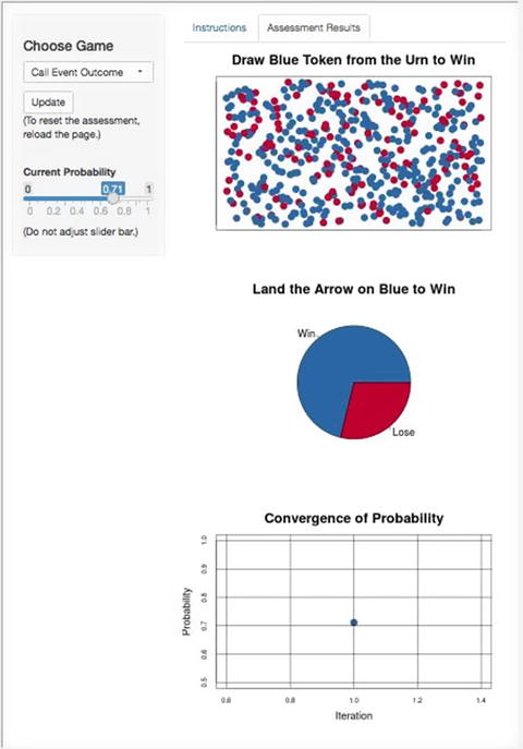
The first iteration, Pr_1 = 0.71, was drawn randomly

The SME chose to call the event so the probability was updated to Pr_2 = (1 + 0.71) / 2 = 0.86

Again the SME chose to call the event so the probability was updated to Pr_3 = (1 + 0.86) / 2 = 0.93

On the fourth iteration, the SME chose to play the lottery, so the probability was then updated to Pr_4 = (0.86 + 0.93) / 2 = 0.89. At this point, the SME was indifferent either to playing the lottery or calling the outcome of the event, so the process was stopped.
The Trouble with Sales Forecasts
Sales forecasts usually depend on the probability of winning a deal (i.e., Pr(win)). Think about the incentives most salespeople have, and ask yourself if the structure of incentives influences their ability to produce unbiased probabilities. Of course it does, but it does so according to the maturity of the salesperson. Younger salespeople tend to be overly optimistic. To correct for this optimism bias, I usually ask a salesperson to assess the probability of losing a deal. The probability of winning is Pr(win) = 1 – Pr(lose). More mature salespeople tend to sandbag their assessments of Pr(win). To correct for this, I ask the salesperson to describe how he or she usually produces a Pr(win) assessment and in what way he or she might adjust it before reporting it to the sales manager. In this case, I just assess the Pr(win). In my experience, however, most salespeople err on the side of optimism. Therefore, it’s usually a good idea to start by asking how the Pr(win) is assessed. If sandbagging is not described, default to assessing Pr(lose).
Sometimes you will need to assess discrete events of more than two possible outcomes. These are the [A, B, C, …] kinds of events. This is the general case of the binary discrete event, and it can be assessed in a similar manner as the binary one. Simply treat the A case as True, and assess its probability. The complementary probability is the residual probability that categories [B, C, …] could occur. Now, assess the probability of B occurring (excluding A from the list). When the SME prefers to call the outcome, use this formula:
instead of
Keep repeating this process until only one discrete category remains. The probability associated with this category will be 1 – (sum of all prior residual probabilities).
Continuous Uncertainties
As I have already alluded , the process of assessing the continuous uncertainty is very similar to that of assessing the discrete uncertainty, except that it usually includes three segments. However, instead of assessing a probability that an event will occur, the SME will be called on to provide an assessment for an 80th percentile prediction interval; that is, the range of values for which the SME posits an 80% degree of belief that will bracket the actual outcome.
- 1.
Start by assessing the P10 value. Tell the SME you are going to find the value for which he or she is indifferent to betting against a lottery with a 1/10 chance of winning or betting that the actual outcome will be less than his or her value. Ask the SME for a ballpark figure, order of magnitude starting point. Let this be P10_1.
- 2.
If the SME prefers the lottery with a 1/10 chance of winning, that means that the P10_1 is too low.
- 3.
Double this number : P10_2 = 2 * P10_1.
- 4.
If the SME prefers betting that the actual outcome will be lower than P10_1 compared to taking the 1/10 chance lottery, that means that the P10_1 is too high. Take half of that number: P10_2 = P10_1 / 2.
- 5.
Update the values on successive iterations such that the last high and last low values bracket the largest movement of the new value: P10_i+1 = (P10_i* + P10_i) / 2, where P10_i* is either the last high if the value needs to move up, or the last low if the probability needs to move down. In other words, you should never go back higher or lower than the last high or last low.
- 6.
Repeat Step 4 until the SME is indifferent to choosing either game to win a prize. This value is the P10 associated with the 10th percentile probability .
- 7.
Repeat Steps 1 through 5, but instead of betting on the actual value being less than the iterated value, the SME will bet on the actual value being greater than the iterated value. The indifference value is the P90 associated with the 90th percentile probability. The P90 should never be less than the P10.
- 8.
The P50 value can be found in much the same way as the P10 value is found in Steps 1 through 5, except here you will use the P10 and P90 values as brackets, and the goal is to find the P50 value such that the SME is indifferent to playing a lottery with a 50% chance of winning (the odds of a coin toss) versus betting that the outcome will be higher or lower than some value between the P10 and P90. Be sure that the SME does not merely evenly divide the difference between the two endpoints.
- 9.
To get an approximately full range (∼99.9%), use the following formulas to find a virtual P0 and P100. These are the endpoints used in the BrownJohnson distribution described in Chapter 3.
If the SME wants to adjust the shape, he or she can do so either by moving the P10, P50, or P90, or by truncating the P0 to a position closer to the P10 or the P100 to a position closer to the P90. Typically, I do not recommend adjusting the P0 or P100 unless there is a systematic reason to impose a constraint, such as the actual value cannot go below zero or it is restricted from going above some number by policy, physical, or logical constraint . Otherwise, let the symmetry in the relative positions of the P10, P50, P90 determine the P0 and P100.
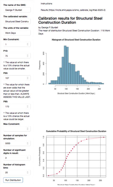
The online continuous uncertainty calibration widget allows you to visualize the range of uncertainty implied by the the 80th percentile prediction interval supplied by an SME. Constraints can be supplied to override the natural P0 and P100 values, if necessary.
It is absolutely imperative that you follow this sequence of events of assessing the outer values first and the interior value last, with no exceptions. The reason for this is that by assessing the outer values first, you will be helping SMEs think about events beyond their initial inclination to consider ; thus, you will be avoiding availability bias. By assessing the inner value last, you will be helping SMEs avoid anchoring. Unfortunately, the all too common practice for producing ranged estimates starts with a “best guess” that is then padded with a ±X% that the SME believes represents a reasonable range of variation without thinking about how probable this range might actually be (it could be either grossly overstated or understated). The best guess is usually anchored in a biased direction, and the padding is just an arbitrary rule of thumb. Biased and arbitrary thinking are not mental characteristics that lead to accuracy in measurements.
Remember, although you are seeking accuracy with the best information you have at hand, you should not try to achieve a false sense of confidence through unwarranted precision by coaxing the SME for narrower ranges rather than wider ones. In fact, the wider the range you assess, the more likely you will take into account events outside the original biased inclination. Furthermore, you should avoid unnecessarily overworking the assessments to get the numbers perfect. The goal is to set bookends to the potential range of outcomes given the quality and limits of the SME’s knowledge at the time of assessment.
Why Don’t We Assess Ranges for Binary Event Probabilities?
- 1.
Probabilities are not intrinsic properties of natural events. Instead, they are subjective expressions about our degree of belief that an event will occur given all the information we can bring to bear on our consideration. If we put a range around the probability that an event will occur or not, we are revealing our internal incoherence about our degree of belief. Then, if we are willing to place a degree of belief around a degree of belief, should we not also be willing to place a degree of belief around each of our bracketing degrees of belief, and so on, and so on? Ultimately, we fall into an infinite regress that prevents us from finding a certain point of indifference between betting on two alternate lotteries of equivalent value.
- 2.
When we assess the range of a continuous uncertainty, we can think of that range as a series of tiny little contiguous, nonoverlapping, mutually exclusive buckets of outcome. If any one of the little buckets occurs, that automatically excludes the other buckets from simultaneously occurring. The probabilities we assess for the three points (0.1, 0.5, 0.9) are actually cumulative probabilities that all the little buckets up to each point can occur. If we were to perform a reverse sum of the cumulative probabilities, the differences would be the probability that a particular bucket would occur or not. Any one little bucket we focus our attention on represents a binary event, which is the limiting case of assessing the probability of any binary event. In the continuous event, we are mapping the point of alignment of all our preassigned intangible degrees of belief on a range of unknown but tangible outcomes. In the singular binary event, we are assessing the unassigned intangible degree of belief that a specific preassigned tangible outcome will occur. In either case, a bucket gets only a single probability for us to maintain mental coherence about measurements we make on the world.
It’s Your Turn
What will the price be of IBM stock (or any other equity you prefer) on a specific date ?
What year did Attila the Hun die? (Answer: 453 CE)
What is the volume of Lake Erie? (Answer: 116 cubic miles; 480 km3)
What is the height of the tallest building in the world? (Answer: Burj Khalifa, Dubai, United Arab Emirates, 828 m, 2,717 ft., 163 floors)
What is the airspeed velocity of an unladen swallow?
Before you attempt to assess any of these, think about specific clarifications and distinctions that need to be made to satisfy the clarity test. Keep track of how often the real value falls between your P10s and P90s.
Document the SME Interview
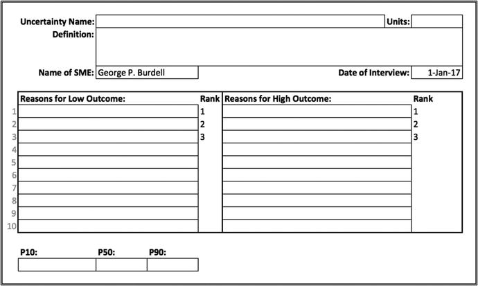
SME interview table
It’s Just an Opinion, Right?
- 1.
Objective : There’s no argument what the process requires, which effectively operates like a method of systematic variation, albeit as a virtual experiment in the mind of an expert.
- 2.
Reproducible : Sufficiently experienced facilitators can assess different SMEs on the same uncertainty and frequently produce highly coherent assessments (although you can sometimes elicit widely divergent measurements, which can indicate that the subject matter is still under contention, or one of the SMEs is not nearly as well calibrated as the other).
- 3.
Transparent : Rationales are clearly defined and documented for later inspection and auditing.
Even though we adhere to an objective process, the subjective nature of the information we elicit should not scare us away from using it. After all, even the best empirical data carry with them many subjective characteristics, namely, the methodological theory that was appealed to for systematically constructing the information, relaxations about the theoretical assumptions that the method specifies, and the subsequent choices that are made about which data are retained and which are discarded, to name a few. Of course, good empirical studies should find ways to eliminate systematic bias and document the ways in which they accomplish that goal or not. When we can use high-quality studies, we should. Unfortunately, though, empirical studies might not even be possible, as in the case of considering the opportunity costs between counterfactual or mutually exclusive hypothetical scenarios. The only way to get unbiased information in those cases (which represents most business case analyses) is to appeal to an omniscient, benevolent clairvoyant. So, in the absence of the best empirical data or omniscient reports from a benevolent clairvoyant, we must start somewhere. Expert judgment provides information that is reasonably constructed, and it is constructed in such a way that we can test the relative sensitivity of dependent figures of merit in our analysis to it. Ultimately, this points the way to the value of information analysis, which sets the research budget for updating our subjective SME prior with, possibly, improved empirical information.