
- 1.
Run the simulation for both decision strategies (or more as indicated) and calculate the mean NPV and NPV cumulative probability distributions. If one of the cumulative probability distributions does not exhibit strict dominance, then we know that sensitivity analysis might be helpful for identifying critical uncertainties.
- 2.
Test the sensitivity of the mean NPV of each decision to the underlying uncertainties using tornado analysis and identify which uncertainties might cause us to regret taking the best strategy (on the basis of expected value) in contrast to the next best strategy.
- 3.
Find the VOI as the difference between the improved NPV by exercising choice based on prior information and the best mean NPV from Step 1.
The Model Algorithms
- 1.
CalcBrownJohnson : Takes p10, p50, p90 assessments from an SME and generates a simulation of samples that spans beyond the p10 and p90 to include the virtual tails.
- 2.
CalcScurv : Models the saturation of uptake into a population using a sigmoid curve. For example, this can be used to model how long it takes to reach maximum saturation into a marketplace.
- 3.
CalcBizModel : The function that represents the business model reflected by the influence diagram.
- 4.
CalcModelSensitivity : Takes a list of uncertainty simulation values and calculates the sequential sensitivity of the NPV returned by the CalcBizModel to specified quantiles (e.g., the p10, p50, p90) for each uncertainty.
Name this file Functions.R, and populate it with the following code.
Note that the business model from the influence diagram is treated as the function CalcBizModel (). The reason I chose to do it this way is that I want to make sure that the logic is consistent among the decision pathways I consider, and I only want to pass relevant information (facts and uncertainties) to the model for the purpose of calculating VOI. If you want access to the intermediate results for other analytic uses and later financial analysis and planning, these values are returned as a list when the function runs. Be aware that because the model is a probabilistic simulation, the values in the returned list are simulation samples; use set.seed() if you want to ensure reproducibility in your results.
You might also notice that while reviewing the functions, and elsewhere in the tutorial, that I depend on for() loops for iteration blocks rather than the often prescribed apply() functions. Yes, the code runs more slowly than otherwise, but in the end I decided that goal of explaining the purpose of the algorithms was clearer using for() rather than apply(). If you are new to R and don’t know what the apply() family accomplishes as a replacement for for() loops, you should learn that quickly. The overall speed of your code will drastically improve.
Next, we need a file that contains our various assumptions and uncertainty assessments. You can name this file Assumptions.R.
Normally, I recommend keeping the parameter data for the uncertainties in CSV files, importing them through the read.csv() function as demonstrated in Chapter 2, and then assigning the uncertainty parameters to each uncertainty with the CalcBrownJohnson() function. In this case, however, the list of uncertainties is short for the purpose of demonstration, so to make things a little simpler and to focus more on the VOI calculation, I took a shortcut.
Now that we have the functional and data pieces in place to initialize and run our model, we can use the following code in, say, Business_Decision_Model.R , to accomplish Step 1 in our solution approach.
Running the prior code gives the following results1 based on our assumptions and logic.
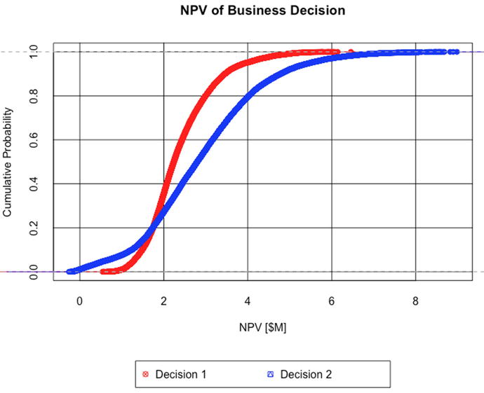
The overlapping cumulative distribution functions (CDFs) for Decisions 1 and 2 illustrate intervals of dominance of one decision compared to another
Decreasing dominance of one decision over another implies that we face increasing ambiguity about which decision to choose clearly. In such cases, we need to know which uncertainties need more attention for determining how to choose clearly. VOI analysis can tell us how much to spend on that attention.
The results in Figure 15-1 show that, given our current state of knowledge about our potential investment opportunity decision choices, we face a dilemma. This dilemma derives from classic finance theory, which tells that, if we are rational, we should prefer those investment opportunities with the highest average (or mean) return and those with the least variance. Here we face the situation in which the best decision based on average return (Decision 2) is inferior to Decision 1 based on its overall variance (Decision 2 is nearly twice as wide as Decision 1 in its full range of potential outcome). Furthermore, we observe that Decision 2 neither strictly dominates over Decision 1 nor stochastically dominates it.
Strict Dominance
There is no sample from the highest valued decision that is lower than any sample from a lower valued decision. Looking at both the probability density function (PDF) and cumulative distribution function (CDF) curves (Figure 15-2), the position of the lowest tail of the highest valued decision would at least be just separated from the highest tail of the lower valued decision.
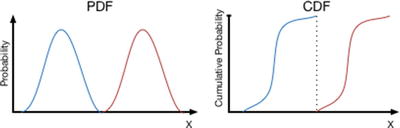
Strict dominance illustrated by the spatial relationship of probability distributions
Stochastic Dominance
The tails of the PDF curves overlap, but CDF curves do not cross over as the highest valued decision remains strictly offset from the lower valued decision across the full range of variation (Figure 15-3).
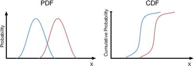
Stochastic dominance illustrated by the spatial relationship of probability distributions
In fact, we observe that the lower tail of Decision 2 crosses over and extends beyond the lower tail of Decision 1 to expose us potentially to a lower outcome than had we chosen Decision 1. The situation we face by our analysis is ambiguous, clearly implying that before we commit to a specific decision pathway, we might want to refine our current state of knowledge. Which of the pieces of information should we focus on? We can develop guidance on how to improve our current state of knowledge with a kind of two-way sensitivity analysis that I have alluded to previously, the tornado analysis.
The Sensitivity Analysis
What we need is a way to prioritize our attention on the uncertain variables based on our current quality of information about them and how strongly the likely range of their behavior might affect the average value of the objective function, NPV . Because we know that the NPV curves overlap, one or more of the uncertainties are causing this overlap as they are the only sources of variation in the model. So, before we go seeking higher quality information about our uncertainties, we first need to understand which of the probable range of outcomes for any of the uncertainties is significant enough to potentially make us regret choosing our initial inclination to accept Decision 2. To accomplish this, we use tornado sensitivity analysis.
Tornado sensitivity analysis works by sequentially observing how much the average NPV changes in response to the 80th percentile range of each uncertain variable. We choose a variable and set it to its p10 value, then we record the effect on average NPV. Next we set the same variable to its p90 and record the effect on average NPV. During both of these iterations, we can set the other uncertainties to their mean value or let them run according their defined variation. Whereas the former approach is generally faster, the latter approach is more accurate, especially if the business model represents a highly nonlinear transform of the inputs to the objective function. If the business model used exhibits strong nonlinearity, Jensens’s inequality 2 effects can manifest.3 The code that I provide here follows the more accurate latter approach. Repeating this process for each variable, we observe how much each variable influences the objective function both by its functional strength and across the range of its assessed likelihood of occurrence.
time -> the time index, year
peak units sold -> uncertainty
time to peak units sold -> uncertainty, years
price -> uncertainty, $/unit
sales, general, and admin -> uncertainty, % revenue
cost of goods sold -> uncertainty, $/unit
tax rate -> % profit
initial investment -> uncertainty, $
discount rate -> %/year
The following code (which I’ve named Sensitivity_Analysis.R) requires that the namespace and sample values of the variables that come from Business_Decision_Model.R be available for use in R’s workspace; therefore, make sure you run Business_Decision_Model.R before running this code.
The results of the sensitivity analysis look like the following tables.
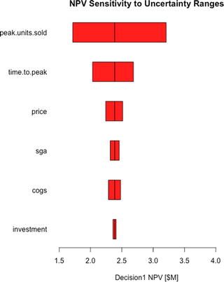
Note that the peak.units.sold variable for Decision 1 returns a value of $1.72 million under the 0.1 column. This is the average NPV of Decision 1 when peak.units.sold is set to its p10 value (e.g., 10,000) while all the other uncertain variables follow their natural variation. Likewise, it returns an average NPV = $3.21 million when it is set to its p90 value (e.g., 18,000) while all the other uncertain variables follow their natural variation. The rest of the table is read in a similar manner.
Please note that a random seed of 98 is used in the Assumptions. (set.seed(98)). Keeping this value set to any fixed value will ensure that you always get the same values between simulation runs of the model. If you change this value, you will observe slightly different values in the reported tables. If you remove the set.seed(98) statement altogether (or comment it out), you will see different values every time you run the model. Just how stable these values remain between runs indicates how sensitive your model is to the noisiness of simple Monte Carlo simulation. Therefore, it is often helpful to run a model several times to get a good feel for this stability (or lack of it), then select a seed value that does a good job of reflecting the ensemble of tests. Otherwise, when you report your values to others who aren’t familiar with the nuances of Monte Carlo simulation, you will face having to explain the nuances of Monte Carlo simulation. Guess how productive that conversation usually is.
Because we already know that Decision 2 has a higher average NPV than Decision 1, we need to know which uncertainties could potentially cause us regret for taking that higher average valued decision. We answer that question by observing which uncertainties cause overlap in the range of NPV between the decisions. If we look down the rows of uncertainties, we see that the two uncertainties that cause such an overlap of value are the peak.units.sold and time.to.peak, as the lowest value of Decision 2 for each of these variables overlaps the highest one for Decision 1.
We refer to these overlapping uncertainties as critical uncertainties because they pose the greatest potential for making us wish we had taken a different route once we commit to the execution of a decision. This is not to say that the other uncertainties are not important and will not need to be monitored once we do commit to a decision; rather, it simply means that for the purpose of making a clear decision now, these critical uncertainties are the greatest contributors to our current state of ambiguity.
Each bar represents the range of variation caused by an uncertainty around the mean value of a given decision .
The order of the uncertainties follows a declining order of importance as determined by the range between the p10 and p90 of each variable.
Overlaying both of these charts provides a better visual cue about which uncertainties should be deemed critical. Here is the code I use to produce the iconic tornado charts for each decision to obtain that visual insight. You can append this to the end of the Sensitivity_Analysis.R file.
Note that we use the rank ordering for Decision 2 as the basis for ordering the display of uncertainty effects across decisions. This will keep the uncertainties across decisions on the same row if it’s the case that the rank ordering differs between decisions. Notice also that we keep the colors consistent with the original CDF charts, and we set the xlimits (xlim = c(min(npv.sens1, npv.sens2), max(npv.sens1, npv.sens2))) for both graphs to comprehend the full range of sensitivity across all the decisions. This latter chart parameter setting ensures that both charts are scaled across the same relative range and that the relative width of the bars for each chart remains consistent.
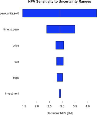
Tornado sensitivity charts for Decision 2 (left) vs. Decision 1 (right)
VOI Algorithms
Following the pattern that I established from the beginning of this discussion, we develop the code for VOI using a simple three-branch decision tree. The purpose is to reinforce our understanding of the method. However, because this method can mask over subtleties in the resultant distributions, we finish the discussion by developing the code that goes much further to preserve those details.
Coarse Focus First
Recall that the CDF curves for the decision values we produced when we first ran Business_Decision_Model.R demonstrated the effect of all the uncertainties acting on the NPV for each decision. Now that we know which uncertainties need our attention for VOI analysis, we need to isolate their effects from those of the other uncertainties. This is easy enough to do now because we already did this in Chapter 14 by computing the reversed decision tree with an analog matrix calculation. Effectively what we’re doing by this is acting as if we have prior knowledge about which outcome will occur more to our favor in many possible future states, and we take the best course of action on each iterated state. The mean value of this new distribution would be the value of having perfect information prior to making a decision. The difference between this value and the highest decision mean value without the prior information is the rational maximum we should be willing to pay for that prior knowledge, the VOI.
Again, run the following Value_of_Information_1.R code after the Business_Decision_Model.R and Sensitivity_Analysis.R to retain the R workspace values.
The final results for the VOI analysis produce the following report.
This implies that if we could buy perfect information about the outcome of peak.units.sold prior to making a decision, we should be willing to spend no more than approximately $300,000 to gain that insight. As we will soon discuss, this value is a coarse focus result. We might be able to improve this value some with a fine focus approach of including more granularity in our uncertainty branches.
We can also interpret VOI in a slightly different manner. Imagine that we are poised at just the point in time before we commit to a decision. In some sense two potential universes exist ahead of each of our decisions, and each universe evolves along multiple potential alternate routes depending on how each conditional uncertainty manifests itself. Suppose that each route has a coordinate pair associated with it indicating the decision and route such that the first possible route for Decision 1 would be (d, i) = (1, 1), and the first possible route for Decision 2 would be (d, i) = (2, 1). The next possible set of routes would be (d, i) = (1, 2) and (d, i) = (2, 2), and so forth for each iteration of our simulated universes. A clairvoyant’s crystal ball makes it possible for us to compare routes (1, i) and (2, i) simultaneously for free with the added benefit of observing only the variation on the NPV of each decision due to the peak.units.sold. Even though Decision 2 has a greater average NPV than Decision 1, there will be some future routes in which the NPV of Decision 1 exceeds that of Decision 2. Given that we prefer futures with higher values and that we are (hopefully) rational, we will always choose the future route (d, i) with the highest value. As a consequence, the resulting value distribution of chosen routes will manifest a higher average NPV than Decision 2. The average incremental improvement in value across those rationally chosen future routes would equal approximately $300,000.
The Finer Focus
The approach I have followed so far relies on the extended Swanson-Megill probability weights to approximate the probabilities of the outcomes of the p10, p50, p90 branches of the decision tree. As approximations, these weights do not strictly conform to the required probability weights of any arbitrary distribution such that its mean and variance are perfectly preserved. The extended Swanson-Megill weights are “rules of thumb” weights for estimating the mean of a distribution, not exact predictors of it.
Of course, the only way to have an exact predictor of an uncertain event’s expected value is to have all the possible samples associated with it (which could be impossible) or to have a symmetry or structure about the event that dictates the expected value, as in the case with fair coins, dice, or a deck of cards. However, we could improve the precision of our calculation simply by using more sensitivity points that represent discrete bins along the distribution of the critical uncertainty instead of predefined quantiles. The bins are analogs of decision tree pathways just as the quantile points were. Given that, we can replicate our matrix approach, but in a more general fashion.
Once our sensitivity analysis identifies a critical uncertainty (i.e., peak.units.sold), we can use it for the more granular analysis. We start by finding the histogram of the critical uncertainty for each decision. (If you do not want to plot the histograms, set the plot parameter to FALSE.)
From these histograms, we need appropriate values from the critical uncertainty to serve as test values to find the contingent NPV values. The plot of the histogram is based on the breakpoints in the domain of the uncertainty, but we don’t need the breakpoints. We need values that represent the bins that are demarcated by the breakpoints. Fortunately, R provides this information in the calculation of the histogram and stores it in the $mid list element.
The histogram returns the following values for the Decision 1 and 2 branch bins:
Note that the first set of bins is longer than the second set.
Next, we need to find a vector of the frequency of the bins in the histograms. We accomplish this by using the $counts values for each bin, then dividing them by the number of simulation samples.
We observe the following frequency values for each bin value.
Each element in the respective vector represents the probability that the given bin, a branch in the decision tree, will manifest; therefore, each of these vectors should sum to 1.
Now we can find the sensitivity of the decision expected NPV by iterating across the uncertainty bins, using each bin as a value for peak.units.sold in the CalcBizModel() function. Make sure to replace the peak.units.sold parameter with a vector of the current bin with a length equal to the sample size (i.e., dec1.uncs$peak.units.sold –> rep(dec1.branch.bins[b], samps)).
We observe the following results :
Now we follow the pattern in the simpler example. Create the MxN matrix of the Cartesian products of the uncertainty branch probabilities.
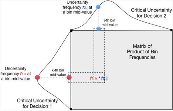
The matrix of the product of the bin frequencies of the critical uncertainty under current inspection is the Cartesian product of those bin frequencies
Next, create an MxN matrix of the values in the bdm1.sens and bdm2.sens vectors. Transpose the values in the second matrix.
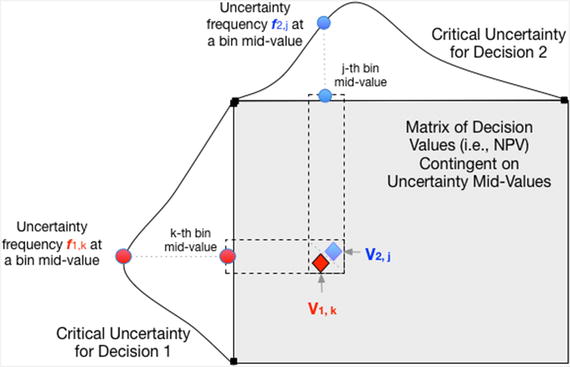
The matrix of the decision values of each possible branch combination that occurs on the outcome of the critical uncertainties’ midvalues
Figure 15-7 illustrates finding the parallel maximum value between these matrices. Recall that this represents knowing the maximum value given the prior information about the combinations of the outcomes of each uncertainty.
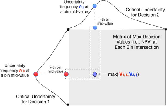
The decision value of each possible branch outcome is found by the pairwise (or parallel) max of each possible outcome combination
Find the expected value of the matrix that contains the decision values with prior information (Figure 15-8). This is the value of knowing the outcome before making a decision.

Find the maximum expected decison value without prior information.
The VOI is the net value of knowing the outcome beforehand compared to the decison with the highest value before the outcome is known (Figure 15-9).
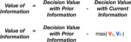
Finally, the VOI is the net of the decision value with prior information and the decision value with current information
This more granular analysis returns the following report:
As in the previous sections, I placed the raw script code for this section in a file called Value_of_Information_2.R. This file should also be run after the Sensitivity_Analysis.R script.
Notice that Prior Information and Value of Information values are a little higher than those obtained by using our coarse focus extended Swanson-Megill branches. Of course, this is due to the fact that our fine-focus use of more branches extends into the tails of the critical uncertainties (which might extend much farther than the truncated inner 80th percentile prediction interval), and we are using a finer distinction in the detail of the whole domain of the critical uncertainty than the ham-fisted discrete blocks of the extended Swanson-Megill.
As you might have inferred, I liken the VOI analysis process to that of using an optical microscope to focus attention on interesting details. Using the extended Swanson-Megill branches is perfectly fine for initially identifying the critical uncertainties as one would use the coarse focus knob. The final approach described here is like using the fine focus knob to gain insights from a more granular inspection of the distribution of probability.
Please note that the approach described in this tutorial applies to calculating VOI on continuous uncertainties by providing a means to discretize the uncertainty into a manageable and informative set of branches. If the critical uncertainty is discrete to begin with, there’s no need to go through the discretization process. One would just use the assessed probabilities for the specific discrete branches.
Is histogram() the Best Way to Find the Uncertainty Bins?
In this last section, I chose to use the histogram() function to discretize the critical uncertainty. This approach is not necessary. In fact, you could use your own defined set of breakpoints that span the full range of uncertain variable behavior, maybe with block sizes of your own choosing or block sizes determined by equally spaced probability. Then you would find the associated frequencies and midpoints within these blocks. Although that might give you a sense of accomplishment of going through the process of writing the code, let me suggest that although VOI is important, it is not a value that needs to be pursued to an extremely high degree of precision. Its purpose is to point us in the right direction to resolve decision ambiguity, to limit the unnecessary expenditure of resources to resolve that ambiguity, and to ensure that whatever resources we do apply, they are applied in a resource-efficient manner. The histogram() function finds an appropriate discretization well enough.
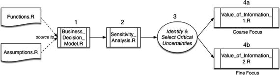
The steps outlined in this chapter to calculate value of information according to the source code files that are used
Concluding Comments
The world is full of uncertainties that frustrate our ability to choose clearly. If we think long enough about what those might be, it doesn’t take long to be overwhelmed. The problem is that we live in an economic universe, a place where there are an unlimited number of needs and desires, but only a limited amount of available resources to address those needs. Finding the right information of sufficient quality to clarify the impact of uncertainties is no less an economic concern than determining the right allocation of capital in a portfolio to achieve desired returns.
An interesting irony has arisen in the information age: We are swamped in data, yet we struggle to comprehend its information content. We might think that having access to all the data we now have would significantly reduce the anxiety of choosing clearly. To be sure, advances in data science and Big Data management have produced some great insights for some organizations that have invested in those capabilities, but whether investments in data science and Big Data programs are mostly economically productive remains an open question.4 The problem, it seems, is that data still need to be parsed, cleaned, and tested for their contextual relationship to the strategic questions at hand before systematic relationships between inputs and outputs are understood well enough to reduce uncertainty about which related decisions are valuable. Not only are we concerned about which uncertainties matter, we now have to ask which data matter, and it isn’t always clear from the beginning of such efforts that if we apply resources to understand which data matter that we will, in fact, arrive at valuable understandings. Regardless, the most important activity any kind of analyst can do to improve the quality of his or her efforts is to frame the analytic problem well before cleaning any data, getting more data, or settling on the best analysis and programming environment. Indeed, solving the right problem accurately is much more important than solving irrelevant problems with high precision or technical sophistication. The advent of the age of Big Data has, perhaps, compounded our original problem.
Every day, I enjoy three shots of espresso. I hope the summarizing shots that follow are just as enjoyable to you in your quest to improve your business case analysis skill set.
Espresso Shot 1
Evaluating VOI helps us address the issues of living in an economic universe. VOI focuses and concentrates our attention on the issues that matter, like an espresso of information. As you noticed in the tornado charts we developed, the width of the bars displays a type of Pareto distribution; that is, the amount of variation observed in the objective measure that is attributable to any uncertainty appears to decline in an exponential manner. The effect demonstrated here did not derive from cleverly chosen values to emphasize a point . This pattern repeats itself regularly. Personally, I’ve observed over dozens and dozens of decision analysis efforts that included anywhere from 10 to 100 uncertainties that the largest amount of uncertainty in the objective is attributable to between 10% and 20% of the uncertainties in question. So here’s an important understanding: Not all uncertainties we face are equally important to the level of worry we initially lend them. The twist of lemon peel is that what we were originally biased to focus on the most actually matters the least.
Espresso Shot 2
The tornado sensitivity analysis delivers a bonus feature. When we compare the charts between important decisions, we see that not all of the most significant uncertainties really matter either. For the purpose of choosing clearly, not every significant uncertainty is critical. Again, from my experience, of the 10% to 20% of uncertainties that are significant, generally no more than one or two are critical.
Espresso Shot 3
The first two shots of information espresso should significantly reduce our worry and anxiety about what can cause us harm and regret as well as reduce the amount of activity we spend trying to obtain better information about them. Now we have a third shot of espresso: When we have identified the critical uncertainties, we can know just how much we should rationally budget to get that higher quality information. VOI analysis, properly applied, should save us worry, time, and money, making us more economically efficient and competitive with the use of our limited resources. As my grandfather used to say, “Don’t spend all of that in one place.” When you are called to spend it, though, don’t spend more than you need to. VOI tells us what that no-more-than-you-need-to actually is.