
CHAPTER 8
Systems Thinking
The leadership we need next cannot try to escape the complexity of the world but has to develop a capacity for effectiveness that acknowledges that the fundamental reality is one of inherent unity. That’s why the primary revolution that we need is a spiritual revolution as opposed to a political or an economic one.
BASICS OF SYSTEMS THINKING
As discussed in Chapter 2, systems thinking is the application of systems theory in organizations. Peter Senge, author of The Fifth Discipline, describes it as “a framework for seeing interrelationships rather than things, for seeing patterns of change rather than static ‘snapshots.’ ” 1
In today’s business environment, the amount of information being created is far greater than at any time in history. And there appears to be no end in sight. The beauty of systems thinking is that it is ideal for managing dynamic organizations that are rich in information.
Mechanics of Systems Thinking
Reality is made up of circles but we see straight lines.
Most businesses have a plethora of sophisticated tools for forecasting and analysis, the results of which are fed into elegant strategic plans.
However, they often fall short in achieving business breakthroughs because they are designed to handle detail complexity. A more pervasive dynamic is one in which the effects are subtle and measured over time; it is called dynamic complexity.
Dynamic complexity takes on various forms. It is present when the short-run and long-run effects of an intervention are dramatically different. Or when an action has one effect on one part of a system and a different effect on another part of the system. Or when obvious actions or interventions produce nonobvious outcomes.
As Senge puts it, “The real leverage in most management situations lies in the understanding of dynamic complexity, not detail complexity.”2 Consider the dynamic interplay of forces in the U.S. economy. As witnessed in the financial collapse of 2008, a new type of investment that entered the system caused an eventual imbalance that wreaked havoc on many innocent parties.
Unfortunately, the typical approach to increasing complexity is increased analysis. Senge points out that “Simulations with thousands of variables and complex arrays of details can actually distract us from seeing patterns and major interrelationships.”3 Most people tend to battle complexity with more detailed solutions. However, this is the opposite of systems thinking.
Senge says “The essence of the discipline of systems thinking lies in a shift of mind. It requires seeing interrelationships rather than linear cause-effect chains, and seeing processes of change rather than snapshots.”4
Feedback Loops
One of the basic principles of systems thinking is feedback. Many Business Intelligence-centric organizations are built around information. The problems arise when information is seen as a static state. According to Meg Wheatley, first introduced in Chapter 2:
Information organizes matter into form, resulting in physical structures. The function of information is revealed in the word itself: in-formation. We haven’t noticed information as structure because all around us are physical forms that we can see and touch and that beguile us into confusing the system’s structure with its physical manifestation. Yet the real system, that which endures and evolves, is energy. Matter flows through it, assuming different forms as required. When the information changes (as when disturbances increase), a new structure materializes.5
The free flow of information is the very lifeblood of organizations. And the larger the company, the more critical it is to keep it flowing. As information moves, it becomes self-generative. As information is sent, received, and processed, new information is created. In this model, feedback loops take on a different meaning. Traditional feedback loops were designed to measure deviations from the norm. The goal was to detect problems or ensure compliance, thereby ensuring the stability of the system. However, to accommodate an adaptive system, positive feedback loops are necessary. These may create short-term disturbances, but they magnify information that creates the impetus to move a system forward.
SYSTEMS VIEW OF BUSINESS ANALYTICS
In the next contribution, Dave Wells, a consultant, mentor, and teacher in the field of Business Intelligence (BI), provides insights into applying systems thinking to BI.
Overview
Many of today’s BI programs focus intensely on analytics. The business wants scorecards, dashboards, and analytic applications, and the technology to deliver them is mature. Still, companies struggle to deliver high-impact analytics that are purposeful, insightful, and actionable. The key to high-impact analytics is a strong connection with cause and effect—the essence of understanding why and deciding what next. Systems thinking offers the cause-and-effect connection. It holds the key to real analytic value that is derived through insight, understanding, reasoning, forecasting, innovation, and learning.
Systems Theory
The key to understanding is to look beyond analytics and think about systems. Not specifically computer systems, although computer systems are one type to which systems theory can be applied. But systems theory applies just as readily to human, organizational, and business systems.
Fundamental truths for all systems regardless of their type include these assertions:
• A system is a collection of interacting parts.
• Behavior of any part is influenced by interaction with other parts.
• A system boundary defines the set of parts that comprise a system.
• A system may interact with things outside of its boundary.
• External interaction is less influential of system behavior than internal interaction.
• Behavior is understood by examining the entire system, not individual parts.
Systems Thinking: Applied Systems Theory
Systems thinking applies systems theory to create desired outcomes or change. It offers a unique approach to problem solving that views problems as part of an overall system. Traditional problem-solving approaches tend to focus on one or a few parts of a system, believing that changes to those parts offer a solution. The systems-thinking approach focuses less on the parts and more on interactions and influences among them as the core elements of problem solving.
Understanding of systems is achieved through identification, modeling, and analysis of relationships and interactions among the parts of a system—a distinctly different and more in-depth analysis than is possible with structural models of a system. Systems modeling is performed by representing the parts of a system and the interactions among those parts.
The most basic concept of systems theory is that a system is a collection of interacting things. The use of the word thing avoids the context-based connotations that might occur with terms such as entity, object, or component.
Things in a system are of many types. They may include (but are not limited to) entities that are familiar to data modelers, objects that are familiar to object-oriented systems analysts, and components as they are understood by software developers. Things in a business system encompass artifacts such as resources, capacities, limits, gaps, goals, desires, actions, results, plans, processes, rules, standards, and much more.
Influence is a behavioral characteristic of interaction. Interaction between two things in a system is directional—one thing has influence on another thing. System behavior is important to understand why things happen in a system and to predict what may happen in the future. Analysis of influences is the key to understanding system behavior.
Systems Thinking Models: Causal Loop Diagramming
Visually representing system behavior is widely practiced in systems thinking with a causal loop diagram (CLD). Causal loop diagramming is a form of cause-and-effect modeling. The diagrams represent systems and their behaviors as a collection of nodes and links. Nodes represent the things in a system, and links illustrate interactions and influences.
Influences are of two types—same direction and opposite direction. A same-direction influence means that the values of two things move in the same direction when change occurs: When employee morale increases, employee productivity goes up. An opposite direction influence means that the values move in opposite directions: When employee stress increases, employee productivity decreases. Exhibit 8.1 illustrates how these two examples are modeled. Note that a plus (+) indicates same direction and a minus (-) is used for opposite direction.
The diagramming technique is called causal loop diagramming because real understanding comes from understanding the system as a whole. Cause and effect is typically not linear; it is circular with a sequence of influences producing a feedback loop. Loops are closed structures that represent a sequence of system interactions without a beginning or an end. A loop may contain any number of interactions greater than one. Feedback is a characteristic of loops in systems.
EXHIBIT 8.1 INFLUENCE AND DIRECTION OF VALUES
Feedback is a process by which the results of an activity or action are returned to the actor in a way that influences the behavior of that actor. Positive feedback occurs when the cumulative effect of all interactions in the loop is one of growth, amplification, or acceleration. Positive feedback loops are often called reinforcing loops. Negative feedback occurs when the cumulative effect of all of the interactions is stabilization or equilibrium. Negative feedback loops are also known as balancing loops or goal-seeking loops.
Exhibit 8.2 illustrates both kinds of feedback loops. Note that the kind of feedback loop—positive or negative—is indicated using a polarity symbol at the center of the loop. Polarity describes the positive or negative feedback property of a loop. Determining loop polarity is relatively easy. Simply count the number of subtractive interactions in the loop. An odd number indicates negative polarity, and an even number, positive polarity.
Individual feedback loops are a step toward understanding cause and effect, but they only scratch the surface. Often the interactions among loops provide real insight into system behaviors by breaking down stovepipe views of the parts of a system. Exhibit 8.3 illustrates this principle with only one minor change to the diagrams shown in Exhibit 8.2. The new model shows a connection between the two feedback loops. Finding these kinds of connections is the first step to developing a holistic view of a system.
EXHIBIT 8.2 POSITIVE AND NEGATIVE FEEDBACK LOOPS
EXHIBIT 8.3 MODELING A SYSTEM
In reality, a system consists of many loops and many interactions among those loops. It is that total system view that helps to achieve depth of understanding and real insight into the behaviors of complex systems. The intersection nodes—those that participate in two or more loops—are the core of system complexity, and they provide the greatest opportunity to discover side effects, hidden influences, and unintended consequences.
Determining the boundaries of a system model can be challenging. Every system is a part of some larger system. Therefore, it is possible to continue modeling infinitely. The time to stop modeling is when enough knowledge and information has been acquired to satisfy the purpose of the model. Stopping too quickly, however, presents a risk that side effects and unintended consequences might be overlooked. Exhibit 8.4 illustrates the nature of this challenge.
EXHIBIT 8.4 SEEKING SYSTEM BOUNDARIES
Systems Thinking and Business Analytics
This section provides only a brief introduction to systems thinking, a subject that is deep, complex, and very much related to business analytics. Only by understanding systems dynamics can the most meaningful measures emerge to deliver analytics that are purposeful, insightful, and actionable. Sometimes business analytics means measuring things, but more often it means measuring interactions and influences.
The discipline of systems thinking includes several archetypes—generic models that represent recurrent patterns in systems. The names of the archetypes are fascinating in themselves: accidental-adversaries, fixes that fail, drifting-goals, tragedy of the commons, and so on. But even more interesting is the clear and certain relationship that exists between these archetypes and the patterns seen in time-series analysis.
Recurring Patterns in Systems
System archetypes—the recurring patterns that are found in systems—show a strong relationship to patterns found in time-series analysis. Virtually every business analytics system analyzes data over time and presents the analysis as time-series graphs. Creating the graphs is relatively easy. Finding meaning in them is frequently more challenging. This is where system archetypes are valuable.
System Archetypes Nine system archetypes are widely recognized in systems theory. Each archetype describes a generic structure that can be generalized across many different settings. The underlying relationships are fundamentally the same regardless of the system or setting in which the archetype is found. Each of the archetypes is described next using causal loop diagramming.
Accidental-Adversaries Localization with system-wide suboptimization typifies the accidental-adversaries archetype. Exhibit 8.5 illustrates the archetype as a causal loop model. It is characterized by:
• Two distinct local reinforcing loops exist, represented by localities X and Y.
• Each locality behaves locally to contribute its own success.
• X locality behaves cooperatively to contribute to the others’ success.
• The two cooperative links create a system global reinforcing loop.
• X’s local actions to contribute to X’s success have unintended consequences that inhibit Y’s success.
• Y’s local actions to contribute to Y’s success have unintended consequences that inhibit X’s success.
• Overall system potential is limited by the effects of unintended consequences of local optimization without global system awareness. The value of the global reinforcing loop is diminished.
EXHIBIT 8.5 ACCIDENTAL-ADVERSARIES CAUSAL LOOP DIAGRAM
As a sociocultural example, consider the conflicting goals and activities of national security versus workforce economics as they relate to U.S. immigration policies. In a more business-oriented scenario, consider an example where two people are managing separate but related software development projects. Cooperatively they have agreed to develop shared and reusable software components, where practical. Yet each of them, when faced with schedule pressures or conflicting needs, chooses to build local custom components.
In behavior-over-time analysis, accidental-adversaries graphs as two activities—X and Y—which both experience accelerating growth early in the time scale. As local optimization limits success potential of both activities, they each decline in the later stages of the time scale. Exhibit 8.6 shows the graphical pattern of accidental-adversaries.
EXHIBIT 8.6 ACCIDENTAL-ADVERSARIES GRAPH
Drifting-Goals Lowering the bar describes the common effect of the drifting-goals archetype. Exhibit 8.7 illustrates the archetype as a causal loop model. The characteristics are:
• Two separate balancing loops exist.
• The two loops intersect at a common gap.
• One loop contributes to the desired state, and another, the current state.
• The gap simultaneously influences action and causes pressure to adjust the desire—in essence to change the goal.
• As the desired state is distorted, the influence on action mutates.
• Ultimately the balance that is achieved has little relationship to the initial desired state.
Consider this scenario: A company is scheduled to negotiate its sales revenue budgets annually. In one year, actual revenue would significantly exceed the budget, creating pressure to increase budget in the following year. The higher budget in the second year caused actual revenue to fall short of budget, creating pressure to reduce the revenue budget in year three. What are the implications of this seesaw budgeting pattern continuing over several years?
In behavior-over-time analysis, drifting-goals graphs as mildly oscillating patterns of both the current state and the desired state. Current state increases slightly over time, as desired state experiences a slight decrease.
EXHIBIT 8.7 DRIFTING-GOALS CAUSAL LOOP DIAGRAM
Eventually equilibrium is reached and both states flatten at a level that is less than the original desired state. Exhibit 8.8 shows the graphical pattern of drifting-goals.
Escalation Competing for dominance best describes the nature of the escalation archetype. Exhibit 8.9 illustrates the archetype as a causal loop model. The characteristics are:
• Two separate balancing loops exist, identified here as X and Y.
• The two loops intersect at a common gap, which is defined as relative results.
• The results of action in each loop influence the desired state of the other.
• The results of action in each loop influence the drive for action in the other.
• The cycle repeats with no apparent end.
The cold war is an obvious sociocultural example of escalation. Competitive pricing is a common business-oriented example. It is common for retailers to advertise that they will match any competitors’ price. What would be the eventual outcome if two retailers each established a policy of beating the other’s best price by 5 percent?
EXHIBIT 8.8 DRIFTING-GOALS GRAPH
EXHIBIT 8.9 ESCALATION CAUSAL LOOP DIAGRAM
In behavior-over-time analysis, escalation graphs as two activities—X and Y—that each grow in a stair-step pattern, with each as the driving force for the next growth step of the other. Exhibit 8.10 shows the graphical pattern of escalation.
EXHIBIT 8.10 ESCALATION GRAPH
Fixes-that-Fail The high cost of the quick fix describes the consequences of fixes-that-fail. Exhibit 8.11 illustrates the archetype as a causal loop model that is characterized by:
• A balancing loop is applied to produce immediate positive results.
• The action of the balancing loop produces side effects in the form of undesirable and unintended consequences.
• A time delay exists between taking action and realizing the side effects.
• The side effects impede the current state from migrating toward the desired state.
Free phone promotions in the wireless telecom industry are a sociocultural example of fixes-that-fail. A business-focused example is a company that is losing customers due to long wait times at the customer service call center. To improve customer retention, the company decides to outsource call center operations. The early result is a visible reduction in wait times and a corresponding reduction of customer attrition due to call center waits. After several months, however, the customer retention rate flattens and begins to trend again toward attrition. What may be the cause, and what fundamental solution may resolve it?
In behavior-over-time analysis, fixes-that-fail exhibit an oscillating pattern of increase followed by decrease. Each of the increases coincides with the introduction of a symptomatic solution. Each decrease that follows is the result of unintended consequences of the fix that become visible only after some delay. It is common that the time intervals between cycles decrease over time and that the amplitude of each wave also shrinks. Exhibit 8.12 shows the graphical pattern of fixes-that-fail.
EXHIBIT 8.11 FIXES-THAT-FAIL CAUSAL LOOP DIAGRAM
EXHIBIT 8.12 FIXES-THAT-FAIL
Limits-to-Success A growth plateau describes the effect of the limits-to-success archetype. Exhibit 8.13 illustrates the archetype as a causal loop model in which:
• A reinforcing loop drives growth of a current state.
• As the current state increases, it interacts with some limiting state in a way that produces a slowing action.
• The slowing action interacts with the current state in a balancing loop that inhibits current state growth and limits the growth effects of the reinforcing loop.
• Rapid growth decelerates, flattens, and may ultimately decline.
One-hour photo developing is an example of limits-to-success where the limiting factor is the emergence of digital photography. Limiting factors may appear in many different forms, including capacity constraints, market saturation, aging product lines, emerging technologies, resource limits, and so on.
In behavior-over-time analysis, limits-to-success exhibit a growth curve that shows early acceleration, followed with deceleration and eventual flattening over time. Exhibit 8.14 shows the graphical pattern of limits-to-success.
EXHIBIT 8.13 LIMITS-TO-SUCCESS CAUSAL LOOP DIAGRAM
EXHIBIT 8.14 LIMITS-TO-SUCCESS GRAPH
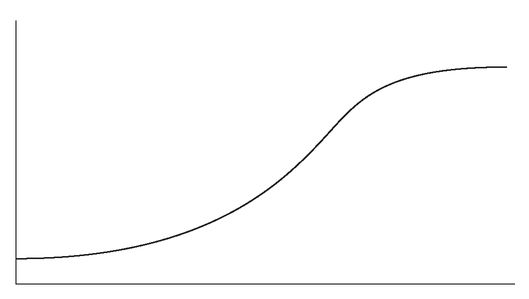
EXHIBIT 8.15 GROWTH-AND-UNDERINVESTMENT CAUSAL LOOP DIAGRAM
Growth-and-Underinvestment A common variation of limits-to-success is called growth-and-underinvestment. In this archetype, the limiting state is created by failure to invest, often due to short-term pressures such as limited capital. As growth stalls due to lack of resources, incentive to add capacity declines, which causes growth to slow even more. Exhibit 8.15 illustrates growth and underinvestment as a causal loop diagram. Note that a complete limits-to-success model is present. Growth-and-underinvestment have the same behavior over time patterns as limits to success.
Shifting-the-Burden The enduring bandage describes the effects of shifting-the-burden. Exhibit 8.16 illustrates the archetype as a causal loop model that is characterized by:
• A short-term solution is implemented that successfully resolves an ongoing problem.
• The short-term solution is implemented as a balancing loop within the system.
• As the short-term solution is used repeatedly, it diminishes the drive to implement a more fundamental solution.
• Over time, the ability to implement a fundamental solution decreases and reliance on the short-term, symptomatic solution increases.
• Ultimately, the short-term solution may produce other side effects that emerge as new problems.
EXHIBIT 8.16 SHIFTING-THE-BURDEN CAUSAL LOOP DIAGRAM
A common example here is overuse of temporary labor to balance workforce capacity with workload demands. Temporary labor satisfies the immediate need to increase capacity. But, when used repeatedly, the percentage of the workforce that is classified as temporary grows, and many “temporary” workers become a permanent part of the workforce. Ultimately issues of Fair Labor Standards Act compliance, benefits eligibility, and such emerge—sometimes resulting in legal action and financial penalties.
In behavior-over-time analysis, shifting-the-burden shows an oscillating pattern of erratic growth of a symptomatic solution. A corresponding (but not always graphed) pattern of oscillating decline in the viability of a fundamental solution occurs simultaneously. Exhibit 8.17 shows the graphical pattern of fixes-that-fail.
EXHIBIT 8.17 SHIFTING-THE-BURDEN GRAPH
Success-to-the-Successful Winners and losers describe the effects of success-to-the-successful, which makes win-win systems difficult to achieve. Exhibit 8.18 illustrates the archetype as a causal loop model that is characterized by:
• Two activities in a system (represented here as X and Y) compete for the same limited set of resources.
• Both activities are represented by reinforcing loops where resources influence success, which in turn influences resources.
• The early success of activity X creates incentive to allocate more resources to X.
• Allocation of resources to X instead of Y increases X’s ability to succeed.
• Allocation of resources to X instead of Y decreases Y’s ability for success.
• Continuation of the cycle reinforces positive results of X and negative results of Y.
• The combined effect of two reinforcing loops moving in opposite directions is a single reinforcing loop that enhances success of X and inhibits success of Y.
• Ultimately X is sustained while Y fails.
EXHIBIT 8.18 SUCCESS-TO-THE-SUCCESSFUL CAUSAL LOOP DIAGRAM
Consider the example of two departments in a company that are competing for priority of information technology (IT) projects. The marketing department needs data and technology to get a 360-degree view of customers and the marketplace and to manage effective marketing campaigns. The research department needs modeling and simulation technology to drive innovation of new products. Both projects are initiated at similar times. In a span of a few months, the marketing department illustrates success with campaign effectiveness metrics. In the same short time span, the research director has only anecdotal justification for the simulation project. The demonstrable success of marketing is reasoned to justify assigning more IT resources to marketing projects, which takes them away from research projects.
Success-to-the-successful graphs as two activities—X and Y—with divergent patterns. The activity to first demonstrate success (illustrated here as X) shows a growth curve, while the other shows a corresponding decline. Over time, the gap widens. Exhibit 8.19 shows the graphical pattern of fixes that fail.
Tragedy-of-the-Commons Shared resource overload is the nature of tragedy-of-the-commons. Exhibit 8.20 illustrates the archetype as a causal loop model where:
• Two activities in a system (represented here as X and Y) depend on a shared resource of limited capacity.
• Both X and Y grow through activity that produces individual gain, as illustrated by two reinforcing loops.
EXHIBIT 8.19 SUCCESS-TO-THE-SUCCESSFUL GRAPH
EXHIBIT 8.20 TRAGEDY-OF-THE-COMMONS CAUSAL LOOP DIAGRAM
• With growth over time, the total activity first approaches and then exceeds the limited capacity of the resource.
• Growth opportunities for both X and Y disappear when the capacity of the resource exceeded.
• Ultimately (especially for consumables) the resource is depleted, which stalls (or even reverses) growth of both X and Y.
Consider the example of a company that depends extensively on the subject and domain knowledge of one person. Initially that person provides valuable knowledge that fuels growth of programs, products, marketing, sales, and quality. As each area grows, demands on the expert increase to the point where he or she cannot keep pace with demand. Ultimately the demands become burdensome, the job becomes unrewarding, and the expert resigns.
In behavior-over-time analysis, tragedy-of-the-commons illustrates three variables. As seen in Exhibit 8.21, two activities—X and Y—exhibit early and steady incline followed by late and rapid decline. The common resource of limited capacity exhibits rapid growth of demand (coincidental with the growth peak of the two activities) followed by very rapid decline.
EXHIBIT 8.21 TRAGEDY-OF-THE-COMMONS GRAPH
Putting the Archetypes to Work The archetypes described in this section are an effective way to gain insight from analytics. It is useful to understand the relationships between archetypes shown as causal loop diagrams and the patterns found in time-series analysis. Whether one is looking at a behavior-over-time graph and asking “Why?” or at a system model and asking “What should I expect?” the archetypes offer a view into the dynamics of systems. Understanding cause-and-effect relationships really is the key to gaining insight through analytics.
Making Cause and Effect Measurable
This section examines stock-and-flow models—the systems thinking tool specifically designed to answer how much.
Stocks and Flows The causal loop techniques described in previous sections help to understand influences among the things in a system. But they make no distinction between the transient things and those things that accumulate. Yet things that accumulate are often the most important to examine when analyzing a system. They are quantifiable and provide the means by which influence can be measured. Understanding the dynamics of things that accumulate in a system is central to modeling and simulating system behaviors. Stock-and-flow models are designed to meet this need.
The things that accumulate in a system are called stocks. A stock is an accumulation of something in a system—either concrete and tangible things (i.e., dollars or widgets) or abstract and intangible things (i.e., knowledge or morale). Tangible stocks are accumulations of consumable resources. Intangible stocks are accumulations of catalytic resources.
A stock changes through the influences of flows. A flow is an action that influences a stock by increasing or decreasing the quantity of the stock. Flows are of two kinds: inflow, which increases the accumulated quantity, and outflow, which decreases the quantity.
The relationships of stocks and flows are graphically represented using stock-and-flow diagrams. Exhibit 8.22 shows a simple stock-and-flow diagram for the accumulation of workforce capacity.
The diagram notation is:
• The stock is illustrated as a rectangle—in this example, workforce capacity based on FTEs (full-time equivalents).
• The arrows indicate two flows: hiring and workload assignment. Inflow and outflow are designated by the directions of the arrows.
• The containers on the arrows illustrate how each flow is quantified—hiring becomes hiring rate and workload assignment becomes workload assignment rate.
• The “clouds” at each end of the diagram mark the boundaries of the problem space. They indicate that the flow hiring rate arrives from somewhere beyond the scope of the diagram and that the flow workload assignment rate travels to a place beyond the scope of the diagram.
The rest of this section builds on the simple example shown in the workforce capacity model. It is important to mention, however, that stock-and-flow models are not always as simple as one stock with two flows. Stock-and-flow sequences may involve more complex and interrelated stocks and flows, as shown in the materials to shipment sequence illustrated by Exhibit 8.23.
EXHIBIT 8.22 STOCK-AND-FLOWS DIAGRAM
EXHIBIT 8.23 COMPOUND STOCK-AND-FLOW SEQUENCE
Measurement of Stocks and Flows Measurement is a key concept of stock-and-flow modeling. Stocks are always measured as units—dollars, items, and so on. In this example, the measurement unit for workforce capacity is employee full time equivalents (FTEs). Flows are measured as rate of flow, which is expressed as units per time period. Flow measures for this example might be FTEs hired per week for hiring rate and FTEs assigned per week for workload assignment rate. Consistency of measurement within a stock-and-flow sequence is important. Measuring workforce capacity as FTEs and quantifying flows as headcounts would make little sense. It would be similarly nonsensical to measure the inflow on a weekly basis and the outflow as a monthly amount.
External influences often affect the rate of a flow. In stock-and-flow modeling, these influences are known as converters. (The term converter may seem odd for this concept right now. However, it is standard stock-and-flow terminology and will make sense later.) Connectors link converters to flows as shown in Exhibit 8.24.
• Labor budget is a converter that affects hiring rate.
• Outstanding orders is a converter that affects workload assignment rate.
EXHIBIT 8.24 CONVERTERS IN STOCK-AND-FLOW DIAGRAMMING
From Causal Loop to Stock and Flow Causal loop diagrams will likely be the initial method to analyze system dynamics, with stock-and-flow modeling used where quantification is needed. A stock-and-flow diagram typically examines a portion of a causal loop model to distinguish stocks from flows and to determine how each is measured. Exhibit 8.25 uses a causal loop model to illustrate how causal loop extends to become stock-and-flow diagrams.
A systematic process of working from a CLD to create stock-and-flow diagrams uses these seven steps:
1. Identify critical behaviors of the system—those that are problematic, under study of analysis, or central to the goals and strategies of the organization.
2. Identify the stocks that participate in critical behaviors of the system—those things that are accumulated in the system upon which critical behaviors are dependent.
3. Name each stock with a term that is quantitative but not comparative. The example in Exhibit 8.25 adds “FTE count” to the name “workforce capacity” to make it quantitative. But it does not say “more workforce capacity,” which is comparative language.
4. Examine every link to each stock to determine if it becomes a flow. If the influence is one that changes the accumulated quantity of the stock, then it is a flow.
5. Add each flow to the diagram expressing the influence as units over time or rate of flow. The example translates “hiring” CLD to “hiring rate” and “workload” to “workload assignment rate.”
EXHIBIT 8.25 FROM CASUAL LOOP TO STOCK AND FLOW
6. Examine each flow in context of the system-wide CLD to identify links that are converters—influences that regulate or otherwise affect the rate of flow. Labor budget and outstanding orders are converters in the example.
7. Mark the boundaries—start and end—of the model.
The act of creating stock-and-flow models from causal loop diagrams also serves to test the causal models and make them more complete. It is common, for example, to discover influences previously not modeled when analyzing rate of flow and identifying converters that affect the rate.
Multiple Stocks and Flows It is possible—even probable—to derive many stock-and-flow sequences from a single causal loop model. When this occurs, valuable insights can be derived by identifying the interconnections among stock-and-flow sequences. Interconnections occur when a flow in one sequence acts as a converter in another sequence. Exhibit 8.26 illustrates an example of interconnected stock-and-flow sequences.
EXHIBIT 8.26 MULTIPLE INTERCONNECTED STOCKS AND FLOWS
Labor budget is a stock whose inflow is labor cost allocation rate. The cost allocation rate is a converter that affects hiring rate, which is an inflow to workforce capacity. Similarly, outstanding orders is a stock with the inflow of order received rate. In both instances the converter link is a flow-to-flow connection. The stock itself is never used as a converter. The result of this analysis is greater insight that may add understanding and detail to the CLD.
Here is where the term converter begins to make sense. The units of measure vary among the three stock-and-flow sequences. Labor budget is measured in dollars. Workforce capacity is measured in FTEs. Outstanding orders is measured as days to complete. A conversion formula is needed to describe the influence of labor cost allocation dollars upon hiring rate FTEs—in other words: How do dollars convert to FTEs? Similarly, there is a need to determine how days to complete is converted to FTEs for the influence of outstanding orders upon workforce capacity.
Business Intelligence Connection
So what does all of this have to do with business analytics? The most obvious connection is the use of stock-and-flow models as the basis for predictive modeling and computer-based simulation. The quantitative nature of these models—stocks measured as units and flows as units per time period—make it practical to define simulation models and apply simulation and predictive analytics tools effectively.
But further consideration suggests that the BI connection is much deeper than simulation and prediction. The power of BI is in the ability to deliver insight, gain understanding, enable reasoning, support planning, and drive innovation.
• Insight is a clear and deep perception of a complex situation or condition—the ability to “see inside” the situation. Insightful analytics are those that create the ability to look inside deeply enough to understand the causes of a situation or condition. Stock-and-flow modeling provides a tool for greater insight through analysis of system behaviors.
• Understanding is the ability to perceive, discern, and distinguish. Distinguishing stocks from flows, units from rates, and causes from effects certainly enhances understanding of how a system behaves.
• Reasoning is the ability to identify root causes, to understand cause and effect, and to logically develop conclusions based on that understanding. Quantifying influences and thinking through questions such as how dollars convert to FTEs undoubtedly advances the capacity to reason about system behaviors.
• Planning is the ability to determine a course of action based on understanding and reasoning. The value of insight is limited unless analytics can help to determine what to do next. By extending understanding and reasoning, stock-and-flow modeling enhances planning capabilities.
• Innovation is the ability to create something new and different—a device or a process—through study and experimentation. Innovation often occurs by combining or connecting existing things in different ways. Stock-and-flow modeling provides a means to study a system in new and different ways. And simulation certainly has a role in experimentation.
The example shown in Exhibit 8.27 is identical to that of Exhibit 8.26 with only one exception. The model in Exhibit 8.26 does not link order received rate to labor cost allocation rate—the converter that is shown as a dotted line.
This example illustrates:
• Insight to see that labor cost budgeting is not currently influenced by the rate at which new orders are received.
• Understanding to recognize that this situation isolates labor budgets from the realities of workload dynamics, which is a fundamental cause of the gap between workload and workforce capacity.
• Reasoning to conclude that the gap will improve if order received rate becomes an influence to determine labor cost allocations.
• Planning that is required to define a course of action through which labor cost allocations are influenced by orders received.
• Innovation to establish a new process through which order received rate influences labor cost allocations, which in turn influences hiring rate and narrows the gap between workload and workforce capacity.
Final Thoughts
Systems thinking is a mature discipline with roots dating back to 1961.6 It is widely known and practiced in many areas where understanding of cause and effect really matters—areas such as manufacturing, process control, industrial systems, and organizational dynamics. Business Intelligence has the same critical need to understand cause-and-effect relationships. It does not make sense for BI practitioners to reinvent the wheel. The BI community needs to learn and adopt the practices of systems thinking. The time has come for systems thinking to become a central discipline of business analysis.7
EXHIBIT 8.27 INSIGHT AND UNDERSTANDING THROUGH STOCK-AND-FLOW MODELING
NOTES
1 Peter M. Senge, The Fifth Discipline (New York: Currency, 1990), 68.
2 Id., 72.
3 Id.
4 Id., 73.
5 Margaret J. Wheatley, Leadership and the New Science (San Francisco: Berrett-Koehler Publishers, Inc., 1992), 104.
6 Randy Urbance, “System Dynamics: Tackling the World’s Complexity.” Available at http://web.mit.edu/esd.83/www/notebook/SystemsDynamics.pdf.
7 For further reading, please see the following books: H.B. Asher, Causal Modeling, 2nd ed. (Beverly Hills, CA: SAGE Publications, 1983); Charles F. Haanel, Cause and Effect (Whitefish, MT: Kessinger Publishing, 2007); Jay W. Forrester, Industrial Dynamics (Cambridge, MA: MIT Press, 1961); David Luenberger, Introduction to Dynamic Systems: Theory, Models, and Applications (New York: John Wiley & Sons, 1974).
..................Content has been hidden....................
You can't read the all page of ebook, please click here login for view all page.