
CHAPTER 4
Full Integrated Risk Modelling: Decision-Support Benefits
In this chapter, we discuss the uses and benefits of full (integrated) risk models. We start with a discussion of their main characteristics, in particular highlighting their differences and benefits compared to risk register approaches, and then provide a detailed discussion of their benefits when compared to traditional static (non-risk) modelling approaches.
(We refer to traditional Excel modelling approaches as “static”. This is not intended to imply that the input values of such models cannot be changed; rather only to indicate that such approaches do not incorporate risk elements as a fundamental part of their conception”; some people prefer the term “deterministic”.)
4.1 Key Characteristics of Full Models
Full risk models are complete models that incorporate the effects of risks and uncertainties on all variables (e.g. prices, volume, revenues, costs, cash flow, tax, etc.); they are simply the counterpart (or extension) of traditional static models, but in which risk and uncertainty are incorporated.
Full risk models contrast with aggregate risk register approaches in several ways:
- The effect on all model variables and on multiple metrics is captured.
- The true nature of the risk is reflected, and time components and dependencies are incorporated.
These points are discussed in more detail below.
In many cases, knowledge of the effect of risks on a range of variables, metrics and performance indicators is fundamental in order to meet the needs of multiple stakeholders. For example:
- A project team may wish to better understand the effect of a delay on resource requirements and on subcontractor arrangements.
- A sales department may be mostly interested in revenue risk, but the manufacturing team may need to focus on the effect of potential breakdowns on volume (which also affects revenue).
- A treasury or finance department may need information on the cash flow, tax or financing profile, or aspects relating to discussion with potential lenders or sources of finance.
- The strategy or business development department may wish to know items that have implications for potential business partnerships.
- Senior management may wish to know about all of the above items (in an integrated, not piece-by-piece or fragmented, analysis), as well as about general project economics and value creation.
Full risk models can also support the development of more enhanced capabilities in areas such as optimisation (or optimised decision-making), as they allow the effect of multi-variable trade-offs to be established. Their use may also be the only way to accurately prioritise risk mitigation actions and general decisions. Similarly, they allow an exploration of issues concerning the structure of individual projects and of business or project portfolios, as in general there will be interactions between the items that need a full risk model in order to be captured.
The true nature of many items is too rich to be captured in risk register approaches, whereas doing so in full models is generally straightforward. For example:
- Items that are best described with simple uncertainty ranges do not fit into operational risk frameworks. For example, the variation in price or sales volume of a product, or the cost of a particular raw material, or a piece of machinery follows general uncertainty profiles (in continuous ranges), and does not usually fit well into a probability-impact framework.
- An explicit time axis is often required, for example:
- In order to calculate items such as net present value (NPV) and internal rate-of-return (IRR), to model cash flow and financial requirements, and to capture project schedules and resource planning issues.
- The time-series development of some items is fundamental to their nature; they may fluctuate around a long-term trend, or have mean-reversion properties, or be subject to multiple random shocks and impacts that are persistent. Some risks may materialise or be active at different points in time (e.g. have an earliest start date, or have a duration), such as for the breakdown of a facility, the entry of a new competitor into the market, a strike by the workforce, the introduction of new technologies, and so on.
- Without an explicit time axis, even basic issues, such as distinguishing between probability-of-occurrences within a period from those over the course of the project, are often overlooked (see Chapter 9 for more discussion of this).
- In general, the use of a single figure to estimate the aggregate time impact would often be inappropriate (as would be done in a risk register approach).
- Dependency relationships between items can be captured in a way that is not possible with risk register approaches. For example:
- A project delay drives investment, production volumes, revenues and some operating costs, with a knock-on effect on profit, taxes and cash flows, and so on.
- The fluctuation in sales prices may be driven by commodity prices, and hence also affect variable costs, with a knock-on effect on margin and subsequent model variables.
- Generally, in models with multiple variables or line items, some are impacted directly by risks whereas others are calculated from other items, which themselves depend on risk impacts. In a standard risk register, impacts are treated as independent, which can lead to incorrect calculations, such as when risks that impact price, volume and launch date aggregate (independently) to result in a negative figure for revenues (in a risk register that aggregates the revenue impact of each risk, for example).
Full models may generally be integrated with a base case model, if one exists (in some cases, only a risk model has been built and no base case has been defined). Often, it is possible to build a switch that governs whether the model's inputs are set to the base values or to the risk values (examples are shown in Chapter 7). Models that are integrated in this way are more likely to be accurate and updated appropriately as the general risk assessment process proceeds.
Risk registers are generally “overlays” that are held separately to a base model, and may be discussed by different groups of people. This separation can lead to base models not being updated even as risk mitigation measures are planned for, and as a project structure changes. For example, plans may be made that require a different product mix, a delayed start time, extra risk-mitigation costs or a different manufacturing location or technology, but these may simply not be reflected in the base model. As a result, it may not reflect the true final structure of a project, and be an inappropriate basis to make decisions; indeed, when used as a reference point for final project authorisation, budget allocations and business planning, the model would be inadequate.
Clearly, the activities associated with building full models are more demanding than those associated with risk register approaches, due to the richness, potential complexity and flexibility requirements that are usually present.
4.2 Overview of the Benefits of Full Risk Modelling
The remainder of the chapter focuses on the benefits of using full risk modelling approaches compared to traditional static ones. The following provides an overview of the main points that are discussed in detail:
- It supports the creation of more accurate models:
- Reflects the uncertainty that is present in the real situation.
- Uses a structured and rigorous process to identify all key risk drivers.
- Allows event risks to be included explicitly and unambiguously.
- Allows for risk-response or mitigation measures, their costs and impacts to be embedded within the base case model.
- Captures the simultaneous occurrence of multiple risks or uncertainties.
- Allows one to assess the outcomes for models whose behaviour is non-linear as the inputs change, or where there is a complex interaction between items in a situation.
- Allows one to capture accurately the value that is inherent in flexibilities and embedded decisions.
- Allows the use of forms of dependency that do not exist in traditional static approaches.
- It enables the reflection of the possible range of outcomes in decision-making:
- Establishes where any planned (or base) case fits within the true possible range of outcomes, and hence the likelihood of such a case being achieved.
- Helps to overcome the structural bias of the “trap of the most likely” (in which static models populated with the mostly likely values of their inputs are often assumed to show the most likely outcome, whereas in fact they may show an output value that is quite different to this).
- Supports the understanding of the implications of other possible base case assumptions on model outputs, as well as the exploration of alternative, or more precise, modelling possibilities of the base case.
- Establishes metrics that are relevant in general decision-making processes, including the economic evaluation of projects and the reflection of risk tolerances, as well as providing a framework to compare projects with different risk profiles, and thus to support the development of business portfolios and strategy.
- Allows for a robust and transparent process to plan contingencies, to revise objectives or modify targets.
- It facilitates the use of more transparent assumptions and fewer biases:
- Allows the base case assumptions (on the value of inputs) to be held separately and to be explicitly compared with the range of their possible values, thus creating transparency and helping to reduce motivational or political biases.
- Supports the balancing and alignment of intuition and rationality in decision-making processes.
- Facilitates the creation of shared accountability for decision-making.
- It facilitates the processes of group work and communication:
- Provides a framework for more rigorous and precise group discussions.
- May allow (apparently) conflicting views on values for assumptions or likely outcomes to be reconciled.
4.3 Creating More Accurate and Realistic Models
This section discusses in detail how the use of risk modelling allows the creation of more accurate and realistic models, as summarized through the key points mentioned above.
4.3.1 Reality is Uncertain: Models Should Reflect This
It is probably fair to say that static models do potentially have a valid role to play in some circumstances, most especially in the earlier stage of considering a new project:
- It is a quick way to explore the basic aspects of a specific situation, and may lead to some valuable insights. For example, an estimate of the order of magnitude of the potential benefits and costs of a project can help to establish whether it needs to be changed in some major structural way, or fundamentally re-scoped, or cancelled.
- Initial attempts to build quantitative relationships between variables will help to drive a thought process about key factors, their interactions and hypotheses that need to be tested, and will generally help to identify whether further research and data gathering is required, and the nature of the information needed.
- It may support the testing of key sensitivities. (However, especially at the early stages of a project, one needs to be mindful of the potential for circular reasoning. The sensitivities shown by the model are a result of the assumptions used and logic of the model, so may be misleading if one concludes that a variable is unimportant in its contribution to risk simply because one has initially incorrectly assumed [due to lack of information at that point] that its possible range of variation is narrow.)
On the other hand, almost any future situation contains risks or uncertainties, and to conduct decision-support analysis that does not reflect this would not seem sensible. In particular, once a basic project concept is considered more seriously (and cannot be ruled out by simple calculations or “back of the envelope” analysis), then it would seem logical to include risks in the analysis: risk modelling “simply” aims to reflect the reality that uncertainties and risks are present, and that an appropriate basis for decision-making should capture their nature and effects, including the potential for their simultaneous occurrence.
4.3.2 Structured Process to Include All Relevant Factors
A formal risk assessment aimed at building a quantitative model has a number of benefits in terms of identifying all relevant factors and includes:
- A high level of rigour and precision in order to correctly identify risks, understand their nature and that of their impacts, avoid double-counting and capture dependencies.
- A focus on the drivers of risk (rather than sensitivity) that will often result in a more accurate and precise capturing of the variation than would a process that is focused only on sensitivity analysis.
4.3.3 Unambiguous Approach to Capturing Event Risks
Risk models can capture explicitly the presence of event risks in a way that is unambiguous. On the other hand, where event risks are present in a situation, the appropriate way to treat them within traditional (static) Excel models is not clear, and is therefore done in a variety of “proxy” ways, resulting in ambiguity, potential confusion or misleading conclusions. In some cases, event risks may not be included at all in a quantitative model: generally speaking, the most likely outcome for any individual risk is its non-occurrence (i.e. the probability of occurrence is less than 50%), so that populating a model with each of its inputs at the most likely value would be equivalent to the risk not happening, so it may as well be left out of the model. On the other hand, if a situation contains multiple such event risks, then from an aggregate perspective, the most likely outcome would be that one or more of them do occur; therefore an approach that ignores them is unrealistic and potentially misleading. Similarly, where a sequence of events is required to happen for an overall outcome to be achieved (such as each of various phases of a drug development needing to succeed for the drug to be brought to market), the most likely case (at each process step) could be for a successful outcome, but in aggregate the success may, in fact, be quite unlikely (see later in this section for an example). As a result of such issues, approaches that are sometimes used involve:
- Including event risks in the model at a fixed value equal to their average probability (or frequency) of occurrence. (This approximation to the average impact may be a reasonable starting point, but as discussed in Chapter 3 may be misleading or inappropriate in many cases, and of course still only provides a static figure. In addition, a model's formulae may require that an input assumption is either one or the other of the valid values, such as if it contains an IF function whose logic is activated one way or the other according to the outcome of the event risk.)
- From a set of possible events, assuming that some will occur and some will not.
- Excluding them from the base model (and the presentation of its results) but listing them separately (e.g. in an appendix of supporting documents), with a brief note under the “model assumptions” that the base case excludes these risks. Thus, in fact, the base case may be extremely unlikely to ever be observed, but this will be hard for decision-makers to assess, and so they are likely to anchor the base case in their minds as if it were a realistic case (which may be acceptable to proceed with as a project), whereas almost all realistic cases may, in fact, be unacceptable if the analysis were correctly conducted.
Thus, in general, when in reality there are event risks in a situation (which is very common), decision-makers are placed in a difficult position to be able to judge the true risks of that situation, unless they are explicitly modelled and their effects captured.
The file Ch4.PriceUpgradePaths.xlsx contains an illustration of an example of such a situation. The context is that a company is facing a rapidly changing market in which any particular product is under price pressure, with an annual reduction in market prices of 5% p.a. expected. However, there are a number of grades of the product that can be sold into the market, with the higher grades achieving higher market prices (at any point in time), but also suffering annual price reductions. The company currently produces only the base grade product, but has plans to invest in research and development in order to develop the (non-public) technology that is required in order to produce the higher grades.
Figure 4.1 shows the company's original plan (contained in the worksheet Original), in which the modelling analyst has not explicitly modelled every process step, but has tried (by using a price increase of 0.5% p.a.) to balance the pressure of the price reduction against the possibility to sell the higher price products; the modest annual increase may be presented as “conservative” if one considers that the higher graded products sell for at least 20% more than the base plan.
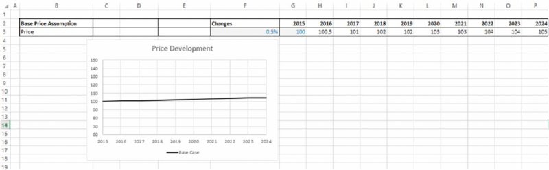
Figure 4.1 Original Model of Price Development
On the other hand, it may make sense to build a model in which one can test the effect of the success of each of the product upgrade processes. The worksheet named Sens (within the same file) contains the calculations in which the price development of each product is explicitly shown. The switches in cells D10:D12 can be used to set whether a particular product upgrade process is successful or not. If a particular upgrade process is successful, the company immediately produces the grade that sells for the higher price.
After consulting internal experts, the modeller is informed that the likelihood of success for the first upgrade is 90%. The second upgrade process can start only if the first one is successful, in which case its probability of success is estimated at 75%, and similarly the third process would have a probability of 60% of success, but can be engaged in only if the second is successful. Not having any risk-modelling tools at his or her disposition, the modeller judges that since the most likely case for each upgrade process is that it will (as an individual process) be successful, it would be inappropriate to assume that some of them are not successful. Indeed, a choice by the modeller to assume that a particular process step would fail will not endear him/her to the organisation or to the particular people responsible for that step, and may not be defensible (since the most likely outcome for that step is its success). Therefore, the revised base case is presented on the assumption that all product upgrade processes are successful, and is shown in Figure 4.2.
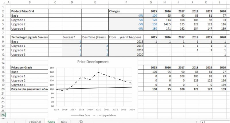
Figure 4.2 Revised Plan for Price Development Assuming Successful Upgrade at Each Step
Clearly, the revised (more detailed) base calculations seem to suggest that there is significant upside to the business case, compared to the original plan in which prices were increasing only 0.5% p.a. However, of course, the issue here is that the uncertainty in the upgrade processes has not been taken into account. The worksheet Risk (in the same file) has the upgraded processes represented as risk events, which are either successful or not (with the given probability, and using the RAND() function to capture this), and captures that a future upgrade process can only be engaged in if the prior one has succeeded. Figure 4.3 shows the results of running a simulation of this in which many scenarios are captured. The graph shows the average price development over these scenarios, as well as the development in the worst 10% of cases.
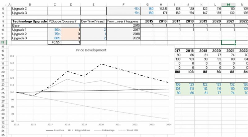
Figure 4.3 Revised Plan for Price Development Assuming Uncertainty of the Success of the Upgrade at Each Step
With respect to the issue of event risks, this model aims to demonstrate the ambiguity that can be present if one does not engage in explicit risk modelling, and the different, possibly misleading, results that can arise in such cases.
4.3.4 Inclusion of Risk Mitigation and Response Factors
The process of risk assessment clearly results in adapting plans in order to respond to or mitigate potential uncertainties and risks. By explicitly including these risk-response measures (including their costs and their impact on the risk items, such as a reduction in uncertainty), one achieves a more accurate model of the reality of the project structure.
Without a formal risk modelling process, it is surprising how often project activity plans are adapted by project teams to respond to risk, but without the base static model being adapted to reflect the cost and effect of these activities. Such a situation is particularly likely to occur due to:
- Lack of awareness. The modeller may be in a different part of the organisation (such as finance), and is not part of the day-to-day workings of the project team.
- Inappropriate base model structure. If the base static model has not been designed to reflect the risk structure of a project (which it almost certainly will not have been without a formal process), then there will simply not be a specific or explicit line item to capture the risk or the effect of the response measures. Thus, the mechanism required to update the model to include the effect of risks and the mitigation measures is not present.
A formal risk assessment process will help to ensure sufficient shared awareness, and support the correct design of a model, so that the effect of response measures can be reflected efficiently.
4.3.5 Simultaneous Occurrence of Uncertainties and Risks
Risk-based simulation captures the effect of the simultaneous variation in all uncertain variables and risks, and in a way that is consistent with their true behaviour. This contrasts with sensitivity and scenario analysis, in which only a limited number of cases are shown, and whose likelihood is not clearly defined or known, as discussed in detail in Chapter 6.
4.3.6 Assessing Outcomes in Non-Linear Situations
Where the output of a model varies in a non-linear way with its inputs, it can be particularly difficult to assess the true output behaviour by using traditional static models or sensitivity analysis. A simple example would be if one were assessing the power output of a wind turbine, which is determined by the wind speed, with (for example) a wind-to-power response curve as illustrated in Figure 4.4.
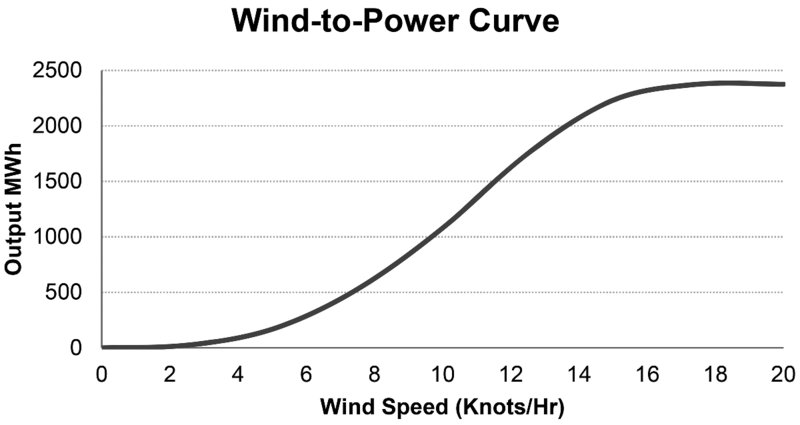
Figure 4.4 Translation of Wind Speed into Power Output
As this is a non-linear curve, if the wind speed is uncertain, it would be challenging to assess the true power output (such as the average) unless many scenarios were run (and their probabilities known). For this reason, simulation techniques are suited to calculate the distribution of possible power output, with each sampled wind speed translating into a particular power output during the simulation.
Figure 4.5 shows the assumed distribution of wind speed in Knots/Hr (a Weibull (2,8) distribution is often used here; see Chapter 9 for details of this distribution), and Figure 4.6 shows the distribution of possible power outputs. (In practice, such a calculation would need to be done for many specific time intervals within the day, e.g. for intervals of 15 minutes, with the Weibull process representing the average wind speed within that interval.)
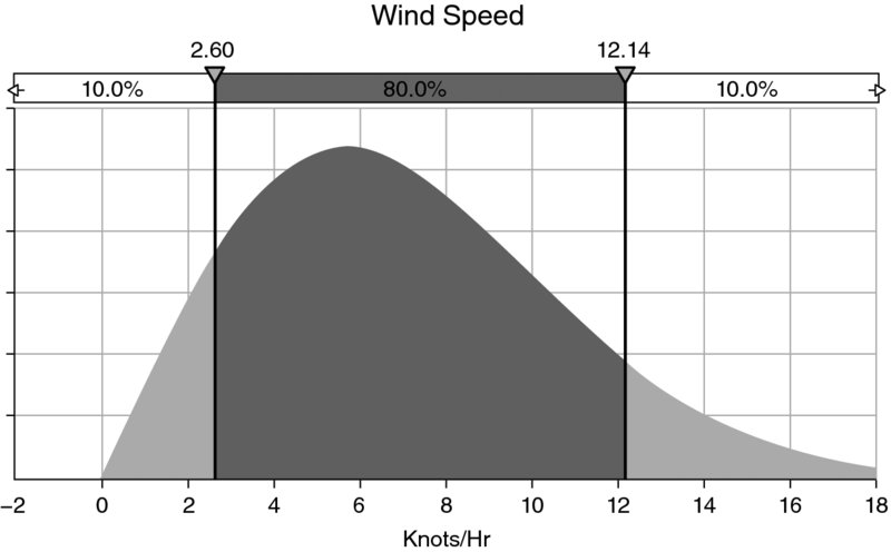
Figure 4.5 Assumed Distribution of Wind Speed
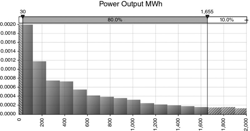
Figure 4.6 Simulated Distribution of Power Output
4.3.7 Reflecting Operational Flexibility and Real Options
Some modelling situations require an explicit consideration of variability for them to be sufficiently accurate or even meaningful. This is especially the case in situations in which there are embedded flexibilities (or decisions that may be taken), but where the particular actions that would be taken depend on the scenario. In general, this is a special case of the non-linear behaviour of models discussed above, in which the uncertainty profile causes a decision to switch results from an interaction of uncertain factors. In such cases, a static model may have very limited relevance, as the values shown in a single case (or in a small set of cases using sensitivity or scenario analysis) will not provide a sufficient basis to accurately evaluate the situation. The general application areas are those that involve contingent claims, liabilities or penalties, as well as real options (i.e. the valuation of flexibility and contingent benefits), such as:
- Government guarantees. A government wishing to encourage private sector investment in a particular industry might provide a guaranteed floor to the minimum prices that the private sector would receive or be able to charge (or a ceiling to the costs that the private sector may face). An example was announced on 21 October 2013 by the UK government, which offered some long-term price guarantees to potential French and Chinese investors in the nuclear energy production sector. In general, in such cases:
- If market prices were always above the guaranteed price level, then the guarantee would turn out not to have any direct value, whereas if market prices were below the guaranteed level, then the government's liability could be large.
- In reality, market prices (or other relevant factors) will develop in an uncertain fashion over a multi-year timeframe, so that they may be below the guarantee level in some periods and above it in others.
- Therefore, the consideration of any single scenario (or even a few selected ones) will not reflect the reality of the situation, and would likely underestimate the benefit to one party and overestimate the costs to the other, or vice versa. To assess the value embedded in such guarantees it would be necessary to capture the payoffs and costs to each party under a wide range of scenarios, as well as to take the likelihood of each scenario into account. For a multi-period situation, and with additional complexities (such as the guaranteed level inflating over time), such a calculation would only be practical with a full risk model.
- Comparing the value in building a mixed-use facility with a dedicated-use one:
- It would generally be more expensive to design, build and operate a production facility that can use a variety of inputs (according to the one that is cheapest) than to do so for a facility that is required to use a single type of input. For example, it would be more expensive to implement the ability to switch to the cheapest in a range of chemical feedstocks (or to different energy types, such as oil, gas or electricity). However, the flexible facility will have lower overall production costs, due to being able to always use the cheapest input. Just as in the above example, the valuation of the benefit achieved by (potentially frequently) switching to the currently cheapest input (and hence to compare this to the operating costs saved) would require the consideration of the full range of scenarios that may happen. In particular, the value of this flexibility will be more in a situation of high variability (volatility) in input prices (especially so if correlations between the price development paths are lower), and the longer the timeframe of consideration. (This “real option” has many analogies to financial market options in terms of the drivers of its value.)
- Similar arguments apply to situations where the end product can be adapted (or optimised) according to market conditions, such as the flexibility to produce different end products for sale (such as a range of chemicals, or a range of vehicles if one has the ability to retool a car manufacturing plant).
- These concepts hold for other types of payoff that depend on the level of an uncertain process or processes, such as profit share agreements, and contracts relating to insurance, reinsurance and general penalty clauses (for example, in service-level agreements).
The file Ch4.OpFlexRealOptions.TripleFuel.xlsx contains an example in which, when designing a manufacturing facility, one has the choice as to which fuel source should be planned to be used: oil, gas or electricity. (To keep the example focused for the purposes of the text at this point, the numbers are only illustrative and are not intended to represent a genuine forecast; we have not considered total expenditure based on volume forecasts, nor do we concern ourselves here with any discounting issues.)
In principle, one could construct a multi-year forecast that calculates the total energy consumption according to each choice, compare the three cases and choose the one for which the costs are lowest. The worksheet Static contains a model in which there are three fuel types whose price development is forecast over a 10-year period. Figure 4.7 shows the calculations, and in particular that the lowest cost choice over the 10-year period would be to use oil (resulting in a total expenditure of $1249 per unit of fuel used, shown in cell C5). In this specific context, we assume that this choice is permanently fixed once it has been evaluated at the beginning of the 10-year period.
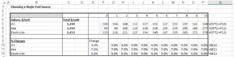
Figure 4.7 Ten-year Forecast of Total Expenditure for Each Fuel Type, Using Static Growth Assumptions
On the other hand, one may have the possibility to build a (more expensive) facility that can be run on any fuel source, so that the fuel used would change each period to that which is cheapest. The worksheet RStaticWSwitch in the same file contains the calculations in which an extra line is added, showing the value of the minimum fuel source in each period, which would correspond to the expenditure in the case that one can switch to that source. This is shown in Figure 4.8. One can see that the best course of action would be to select to use gas for three periods before switching to oil at the beginning of the fourth period and then to always use oil thereafter. In this case, the expenditure over 10 years would be $1234 per unit, or a saving of $15 compared to having no switching possibility (cell C8).
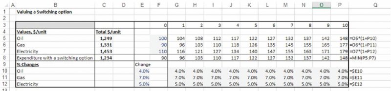
Figure 4.8 Ten-year Forecast of Total Expenditure for each Fuel Type, Using Static Growth Assumptions and Including a Switching Option
However, the model does not yet fully capture the effect of uncertainty, because the number of switching possibilities is limited to at most two (as the price change assumptions apply for the full model timeframe); if price changes are uncertain within each period, then there are many more switching scenarios. The worksheet RiskWSwitch includes a forecast in which the uncertain development of each is taken into account (this uses a normal distribution, discussed in detail in Chapters 8, 9 and 10). By pressing F9 to recalculate the model, one sees many different scenarios: in some cases, the source that is initially cheapest may remain so, whereas in others, there may be frequent switching, so that the savings would be higher. A simulation can be run to capture the average saving over many scenarios. Figure 4.9 shows the results of having done so. The results suggest an average expenditure of approximately $850 per unit (cell D8), or a saving of approximately $400 per unit compared to the original case in which there was no switching possibility; cell R8 contains the calculation of the savings made by the use of the switching approach compared to the next best possibility.
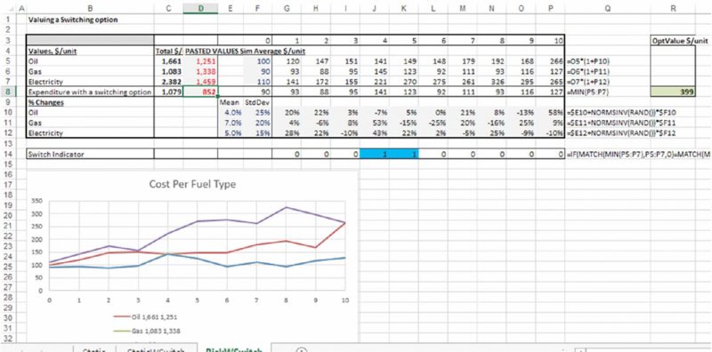
Figure 4.9 Ten-year Forecast of Total Expenditure for each Fuel Type, Using Uncertain Growth Assumptions and Including A Switching Option
The example shows once again that (although the core aspect of the model design is the creation of the extra line item to incorporate the switching possibility) it is the presence of uncertainty that creates most of the value in the real-world situation. On the other hand, without any consideration of the uncertainty, both the possibility to consider the switching option and the utility of pursuing this as an option to be analysed could have been overlooked, with the result that the potential benefits of the operational flexibility would not have been considered or exploited.
4.3.8 Assessing Outcomes with Other Complex Dependencies
In general, when a model's logic is not simple (even the presence of IF or MAX functions, or other non-linear behaviours is sufficient), and especially when certain calculation paths are only activated by a change in the value of multiple items, it can be challenging to use intuitive methods to assess the sensitivity of output to input values. In such contexts, the use of uncertainty modelling can be extremely valuable. Examples include:
- Where there are operational flexibilities that need to be captured in the evaluation of a project (as shown above).
- Where only the joint occurrence of a number of items would cause a product to fall below a safety limit, one would need to capture this by checking this condition in the model. In a simple sensitivity approach, in which only one or two factors would be altered (e.g. switch variables to turn a risk on or off), such scenarios may never materialise, potentially resulting in a modeller overlooking the need to check whether failure can occur at all.
- In project schedule analysis, an increase in the length of a task that is not on the critical path may have no effect on the project's duration, whereas an increase in the duration of activities that are on the critical path would increase the project's duration. For some tasks, an increase in its duration may have only a partial effect (for example, if the path on which the task lies becomes the critical one only after the task length has increased by a certain amount). Additionally, when there are multiple variables (or items that affect task durations) that may change at the same time, establishing the overall effect of these on the project's duration is difficult, unless an uncertainty modelling approach is used.
For fairly simple situations, schedule models can be built in Excel. In particular, where a project consists of a simple series of tasks (in which each always has the same predecessor and successor), and where task series occur in parallel with no interaction between them, then Excel can be used to determine project schedules: the duration of a series of tasks is the sum of their durations (including the duration of planned stoppages and other non-working time), and the duration of task series conducted in parallel is the maximum of such series. One advantage of using the Excel platform in such cases is that cost estimation can be linked to the schedule.
The file Ch4.ProjectSchedule.xlsx contains an example; Figure 4.10 shows a screen clip. There are three main task series, each consisting of three tasks. Within each series, the tasks are performed in sequence, so that the series duration is the sum of the duration of its tasks (e.g. cell J4), but the task series are in parallel, so that the total project duration is the maximum of these sums (cell J17). There is also a switch cell to choose between the risk case and the static case; in the case shown, the model is shown at its base values (in column J). Column G shows the probabilities for the third task series, which consists of event risks, whose occurrence is captured in column I (since the model is shown at the base case, these event risks are not active within the calculations in column J).
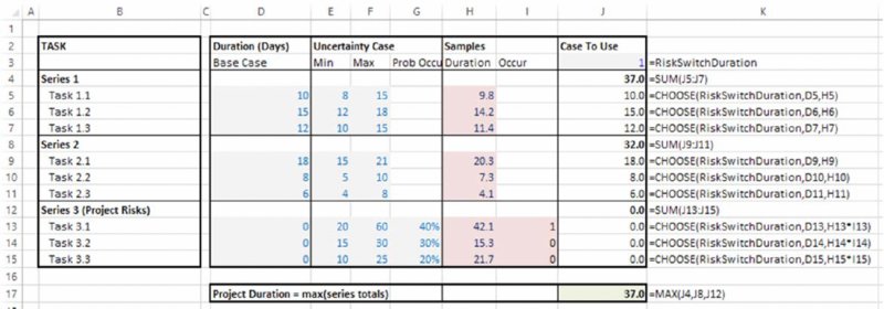
Figure 4.10 Model of Project Duration (Base Case View)
Note that since the model is built in Excel, it is relatively straightforward to add a cost component, in which costs are determined from durations, as well as having their own variability. Figure 4.11 shows the cost component of the model, in which total costs for each activity are calculated as the product of the duration (in days) and the cost per day. The cost per day also has a switch to be able to use either fixed values or base case static values.
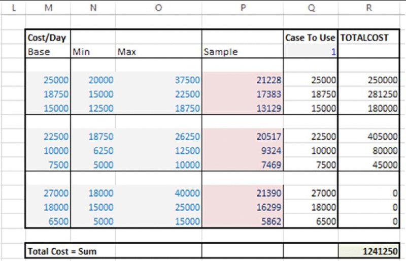
Figure 4.11 Model of Project Cost (Base Case View)
A simulation can be run to calculate the distribution of the duration, and of the costs, of the project; see Figures 4.12 and 4.13, respectively (once again the simulation is run using @RISK in order to use its graphics features, but the reader may use the tools of Chapter 12 instead in order to do so purely in Excel/VBA).
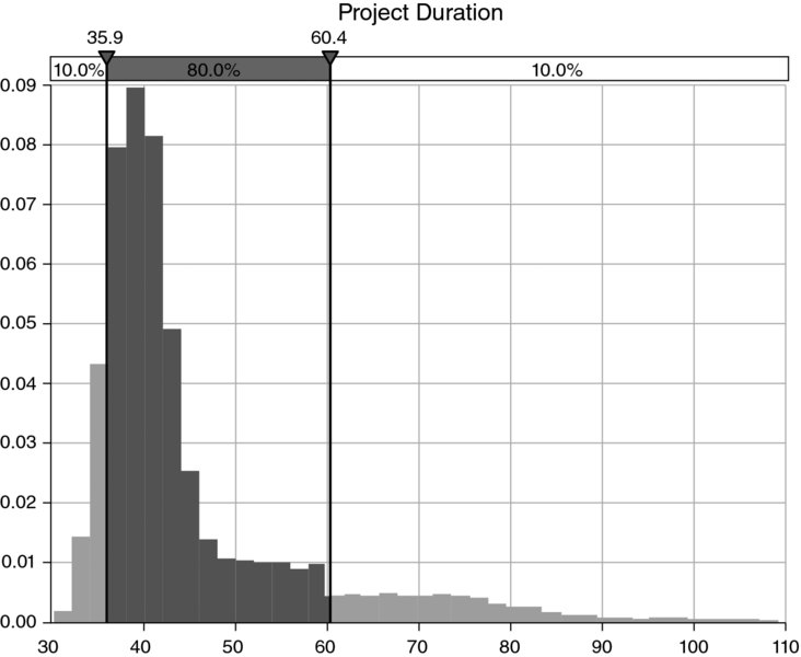
Figure 4.12 Simulated Distribution of Project Duration
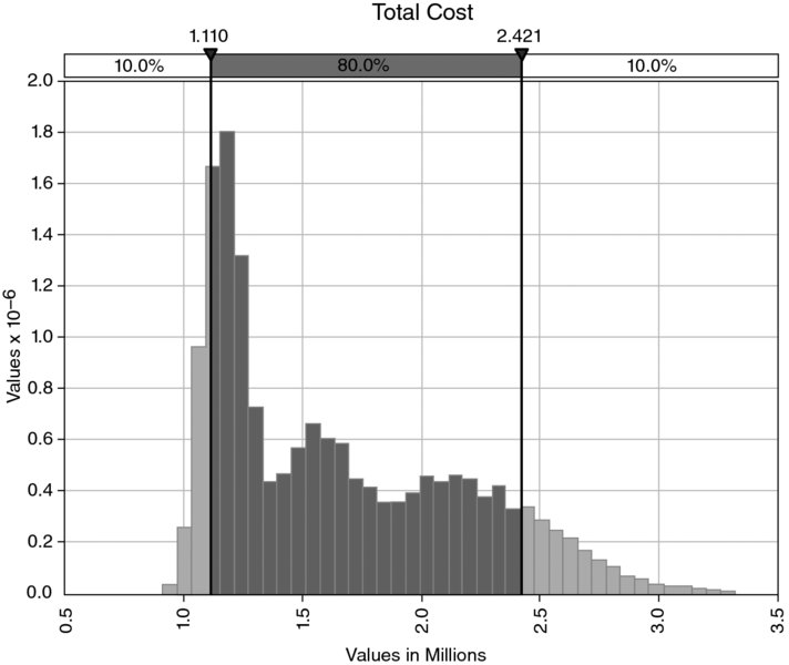
Figure 4.13 Simulated Distribution of Project Cost
Finally, a scatter plot can be produced showing the cost range for each possible duration; see Figure 4.14.
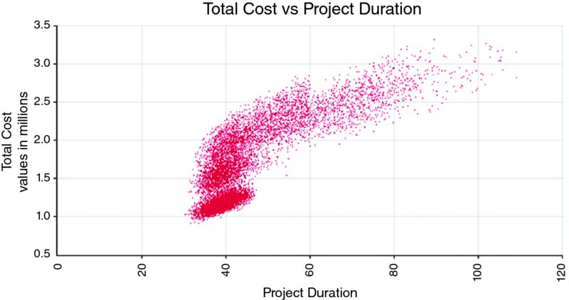
Figure 4.14 Simulated Distribution of Project Duration Against Cost
As a final note with respect to this area of application, the more general challenge in such project schedule analysis is where the critical path changes in more complex ways as task durations vary, so that the formula that defines its duration is too complex to capture in Excel. This is one of the reasons for using the MSProject tool within @RISK (see Chapter 13).
4.3.9 Capturing Correlations, Partial Dependencies and Common Causalities
Risk models can capture relationships between input variables that are not possible in traditional models:
- In a traditional model, as soon as one input is made to depend on another – such as volume decreasing as price increases – then this second variable (volume) is no longer a true input: it becomes a calculated quantity, with the inputs becoming price and the scaling factors that are required to calculate volume from any given price.
- In a simulation model, there can be relationships between input variables (distributions), such as conditional probabilities, partial dependencies, correlations (correlated sampling), copulas and others. This provides for a richer set of possible relationships that generally enable one to more accurately capture the reality of a situation (see Chapter 11).
- In addition, the risk assessment process will also help to identify common dependencies that are often overlooked if one uses a sensitivity analysis approach (see Chapter 7).
4.4 Using the Range of Possible Outcomes to Enhance Decision-Making
The use of risk modelling (including the simultaneous variation of multiple risks) provides one with an estimation of the distribution of possible outcomes. From this, one can find the likelihood that any particular case could be achieved (for example, that costs will be within budget, or revenues less than expected, and so on). In addition, the variability of the outcome is also relevant for real-life decision-making since risk tolerances (preferences or aversion) need to be able to be reflected; we may not, in reality, wish to continue with a project that has only a 50% chance of success, or that will go over budget in 50% of cases.
Generally, of course, one implicitly assumes that if a static model uses “reasonable” assumptions for input values then the output will also show reasonable values. Indeed, the phrase “garbage in, garbage out” is often used to express the importance of using reasonable estimates of input values, and of course it is important to pay attention to the selection of base case values (e.g. perhaps using “best estimates”). On the other hand, statements such as the following are either assumed or implicitly believed:
- “There is essentially a 50/50 chance of deviating either side of the base case.”
- “If a model's inputs are at their most likely values, then the model's output is also its most likely value.”
- “If a model's inputs are set to be their average (or mean) values, then the model's output also shows its average (or mean) value.”
- “As long as the inputs are not too optimistic/pessimistic, then the output will be a reasonable representation of reality.”
- “Any optimism and pessimism in the input assumptions will more or less offset each other.”
In reality, none of these statements is generally true, although they may each be true in specific circumstances, depending on both the nature of the uncertainty and the logic contained within the model. In general, the output case shown by a model will not be aligned with the input case definitions (in terms of definitions or the placement of each value within its own range). This potential non-alignment is driven by:
- Non-symmetry of uncertainty. The driving forces that can cause random processes to be non-symmetric in practice are discussed later in the text.
- Non-linear model logic. Once models contain even relatively simple non-linear behaviours, such as IF statements, then it becomes very difficult to make any general assertion about the position of a single scenario with the full range of outcomes.
- Event risks. For some individual event risks, the most likely outcome may be that they do not occur (for probabilities less than 50%), whereas when there are several such risks within a model, the most likely outcome is generally that at least one would occur.
(Thus, alignment is to be found in special cases, such as models that are linear and additive. In such a model, the average or mean values for the inputs translate into the output's average, and absolute best and worst cases are also each aligned.)
Whilst it may be intuitively clear that if base case values are slightly biased or imperfect, then the output will be so, what is much less clear is the strength of the effect, which can be very significant in the presence of multiple uncertain variables. In effect, these are structural issues (or biases) that are often overlooked, and provide a compelling argument to use risk modelling techniques and conduction simulation: Einstein's comment that “a problem cannot be solved within the framework that created it” is pertinent here.
These issues are examined further in this section.
4.4.1 Avoiding “The Trap of the Most Likely” or Structural Biases
Where each input value of a traditional (static) Excel model is chosen to be the most likely value of its underlying distribution (a “best guess”), it is often believed that the base case is “non-biased”; when required to select only a single figure as a fixed estimate of the outcome of an uncertain process, this figure would seem appropriate (as any other figure is less likely to occur). However, in such cases, the output that is displayed in the base case may, in fact, be quite different to its true most likely value; indeed, the likelihood of its being achieved could be very low (or very high).
As a simple example, assume that one regularly takes a journey which, based on experience, takes 25 minutes in 70% of cases (the most likely case), but which is sometimes longer (35 minutes in 20% of cases), and sometimes shorter (20 minutes in 10% of cases). If one is planning how much time will be spent travelling over the next 10 days (perhaps one reads during the journey and wishes to plan one's reading schedule), then one could add up 10 sets of 25 minutes, giving 250 minutes. This corresponds to building an Excel model, with a row for each of the 10 days, and populating each row (day) with its most likely value. However, it is intuitively clear that the average (and perhaps the most likely) total time will be more than the base figure of 250 minutes, since the journey lasts 10 minutes longer in 20% of cases, but only 5 minutes less in 10% of cases; these do not offset each other. Figure 4.15 shows the results of running a simulation model using @RISK to generate many scenarios, from which one sees that the base case of 250 minutes is exceeded with a frequency of approximately 80%; indeed, in around 25% of cases, the total journey time is more than 275 minutes (so that over the course of 10 days, one has used the equivalent of an extra 25-minute journey). Moreover, over the course of 100 days (shown in the graphic on the right), there is essentially no realistic chance that the total journey time would be 2500 minutes or less, and that the most likely journey time is approximately 2650 minutes, not 2500.
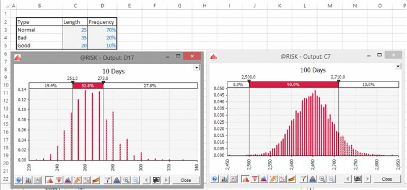
Figure 4.15 Simulated Total Travel Time for 10 Days and 100 Days
Of course, the same principle would hold when applied to other situations that are logically similar, such as estimating the costs for a project by adding up the individual components; if each component is uncertain and with a balance of risk to the upside, for example, then the likelihood of the final outcome being below or at the sum of the base values is low.
Thus, the “trap (or fallacy) of the most likely” refers to the fact that models calculated using the most likely values of the inputs will often not show the most likely value of the output (although it is often implicitly believed that they do). Thus, it is clear that decision-makers may often be given misleading information; the base cases referred to for decision-making purposes may, in fact, represent scenarios that are quite unlikely.
(The issue as to whether the most likely case of the output is a relevant decision-making metric is discussed in Chapter 8.)
4.4.2 Finding the Likelihood of Achieving a Base Case
In a sense, it is perhaps unsurprising that decision-makers have often grown sceptical as to how much weight to give to the numerical side of decision-making when based on the output of static models, and place a large amount of importance on intuitive, heuristic or judgemental processes: the process used to provide them with information is structurally flawed. On the other hand, if these biases and misleading results could be overcome, then numerical calculations should be able to have more credibility within decision-making processes.
In many cases, the inputs used in a base case model may be biased in several ways:
- Structural biases, meaning that it may show base case output values (or scenarios) that are highly unlikely, even as project teams have worked hard and made genuine “best efforts” to populate the assumptions with “non-biased” inputs.
- Motivational or political biases, such as the desire to have the project authorised.
The cumulative effect of several “small biases” (or “white lies”) may be stronger than one's natural intuition would expect, so that establishing the likelihood of achieving a particular base case is perhaps the single most important benefit of quantitative risk modelling in many situations.
(Note that we are assuming that a static base case exists, which is generally the situation. In principle, one could argue that base cases should not be needed once inputs are represented by distributions. For example, after simulating a risk model, one may decide that the P75 of the output should be considered to be the base. However, in practice, input base values are required for line items that correspond to those against which plans are made, or resources or budgets committed to. For a given output figure, such as a P75, there is no one single input combination that will produce such a figure, and hence some form of base case is usually required.)
One can explore (using simulation) the issue of how a particular selection of base case affects the position of that case within the range of the true output. Figure 4.16 shows an example of a cost budget with 10 items, each of which has a possible range (for the sake of presentation only, we assume that their parameter values are all the same). For simplicity here, we assume that the ranges are symmetric, and that each range is described by a PERT distribution (relevant details are covered in Part II; here we are concerned only with the concept), as shown in Figure 4.17. Thus, if the base case for each input were assumed to be slightly optimistic (i.e. lower than average cost), for example its P40 value (9785), then the sum of these values shown in the base model would be 97,850 (as shown in Figure 4.16).
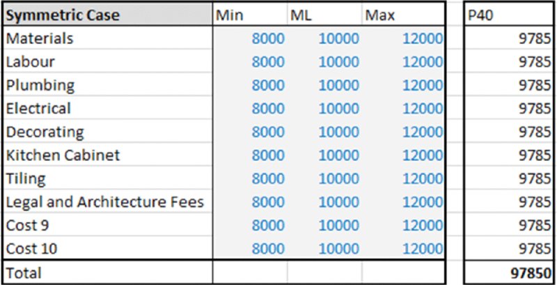
Figure 4.16 Cost Budget with Each Base Case Value Equal to the P40 of its Distribution
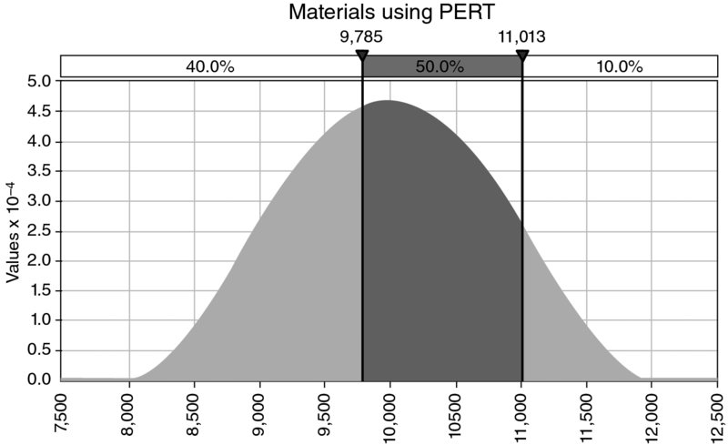
Figure 4.17 Assumed Cost Distribution for Each Item
On the other hand, Figure 4.18 shows the result of running a simulation to work out the distribution of total cost, from which one sees that the figure 97,850 is approximately equal to the P20 of the distribution, and hence is even more optimistic.
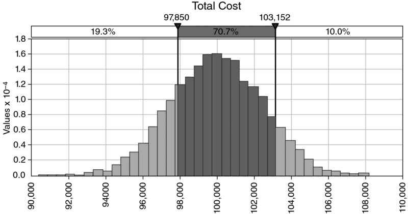
Figure 4.18 Simulated Distribution of Total Cost
More generally, one can compare cases for how various input assumptions would map to various outputs. Figure 4.19 shows how particular assumptions for base values (as percentiles of their distributions) would map to the percentile of the output. One can see that P50 inputs map to P50 outputs (as we have assumed symmetric distributions), but that optimistic input percentiles (below P50) map to lower percentiles of the output (and hence the output is even more optimistic than is the input), whereas pessimistic inputs (above the P50) create even more pessimistic cases in the output.
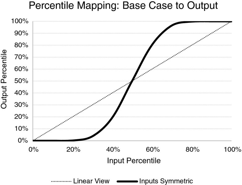
Figure 4.19 Mapping of Base Case Percentiles to Output Percentiles for 10 Symmetric Inputs
When the input distributions are non-symmetric, the same basic principles apply; however, the cut-off (or equilibrium) point (which is, in fact, the average) has a different percentile; for a positively skewed distribution, a P50 input would be optimistic (and lead to an even lower percentile for the output than in the symmetric case). This is shown in Figure 4.20, in the case where the maxima of the distributions in the examples were 15,000, rather than 12,000.
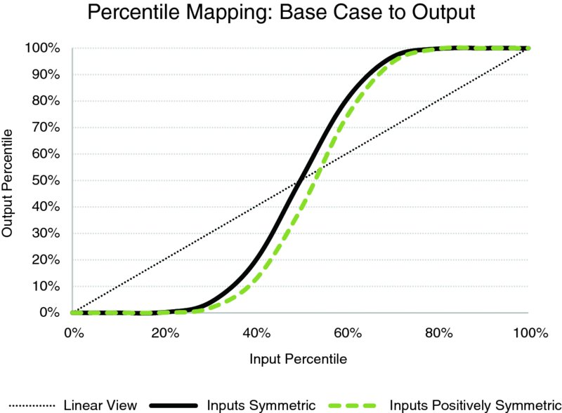
Figure 4.20 Mapping of Base Case Percentiles to Output Percentiles for 10 Symmetric and Non-symmetric Inputs
Clearly, the precise outputs shown in charts such as Figures 4.19 and 4.20 depend on the nature of the model and on that of the uncertainties. For example, the diagonal line effectively corresponds to a model with one variable, so that there is a direct correspondence between the input and output. Thus, the line becomes narrower and steeper if more cost elements are added to the model (all other things being equal). Figure 4.21 shows this as the number of items in the model changes (for one, two, five and 20 items). For models with more variables, since the curve is steeper, for base cases toward the middle of the range (i.e. ones that could be considered “reasonable” or not excessively biased), even a small change in the chosen case described by (all) the input values would have a significant effect on the percentile of the output.
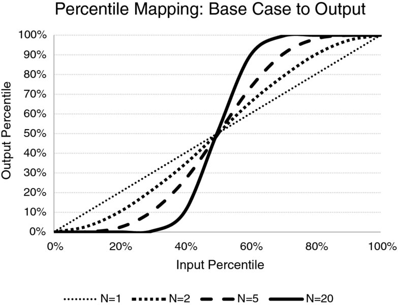
Figure 4.21 Mapping of Base Case Percentiles to Output Percentiles for Various Numbers of Symmetric Inputs
The basic principle at work in this situation is that of diversification. For example, with reference to the case in which there are only two uncertain items, and for which the base case for each input is defined as its P90 (so that it would be exceeded in 10% of cases), then for the sum of the two uncertain processes to exceed the sum of these two figures, at least one of the uncertain values has to be at least equal to its P90 value (which happens only 10% of the time); in the majority of such cases, the second variable will not be sufficiently high for the sum of the two to exceed the required figure (because in 90% of cases, the value of the second one will be below its own base figure). Roughly speaking, the base case (sum of the P90s) may be thought of as being the P99 of the sum; in fact the percentage would be lower (in Figure 4.21, it is approximately 97%) because there will be cases where one process is above its own P90 by a reasonable margin, whilst the other is only slightly below its own P90, so that the sum of the two is nevertheless above the sum of the individual P90 figures.
A number of other points are worthy of note here:
- The notions of optimism and pessimism mentioned above depend on whether a higher percentile is good or bad from one's perspective. For example, whereas in cost contexts, an assumption of low cost would be optimistic, in a profit context it would be pessimistic. Thus, in the case of the estimation of uncertainty of oil and gas reserves, where P50 estimates for individual assets may be used as a base, and where the distribution of reserves is often regarded as lognormal (and therefore skewed to the right; see later), the sum of a set of P50 values will be less than the true P50 of the sum. Thus, a simple aggregation of base figures would underestimate the true extent of reserves, and thus is a pessimistic estimate (so that on average, in reality, there will be more reserves than originally expected, even without further technical advances or new enhanced recovery procedures). Similarly, the summation of the P90s (or P10s) of the reserves estimated for different assets does not provide the P90 or P10 of the total reserves.
- In general, the set of values used in a base case will be some mixture of items: some may be the most likely values, some may be optimistic and some pessimistic. Simulation techniques can be used to assess the consequences of these various assumptions in terms of how the shown base case output relates to its position within the true output range. Indeed, such an assessment may help one to avoid undertaking activities that in fact have little chance of success, even where the “base case” seems to suggest a reasonable outcome.
4.4.3 Economic Evaluation and Reflecting Risk Tolerances
The knowledge of the distribution of outcomes can assist in many ways in project evaluation and associated activities:
- The average outcome is the core reference point for economic valuation (such as the average of the net discounted cash flow), as explained in detail in Chapter 8.
- In some practical cases, the average will not be so relevant, but other properties of the distribution of outcomes are required in order to reflect risk preferences (corporate and personal) in the decision. This applies, for example, to the economic evaluation of projects that are large and cannot be regarded as repetitive decisions, or where failure could result in bankruptcy of the business or a loss of status for the decision-maker. In addition, in non-financial contexts, such as schedule analysis, the average (e.g. time to delivery of a project) is often not as relevant as other aspects:
- Often, very senior management may be willing to take more risk to achieve corporate objectives, as long as this risk is well managed and the risk exposure understood.
- More junior management will typically be more risk averse, and may consider that the occurrence of a loss would not be acceptable to his or her career prospects, and hence would tend to reject the same project.
- These differences in risk preference may lead to apparently inconsistent decision-making according to which level of an organisation is involved, but this can partly be offset by a transparent approach to risk evaluation and the setting of more explicit risk tolerances that quantitative assessment allows.
- To compare projects with different risk profiles. A project with a more positive base case but also higher chance of a severe failure than another (i.e. higher risk reward) may be favoured (or not) depending on the context and its potential role within a portfolio of other (perhaps low risk) projects.
- To identify early on projects that may be unsuitable due to their risk profile. In particular, the early elimination of potential “zombie” projects is a key objective. These are projects that in reality have little prospect of success, but become embedded in the organisation if not stopped early; vested interests start to grow, including those of the original project sponsors who may find it difficult (and career limiting) to change their position on the benefits of a project. The pursuit of such projects can require much investment in organisational resources, time and money before (perhaps) being stopped at a very late stage and with great controversy (e.g. at the final authorisation gate or only when the main project sponsor leaves the company).
- Incorporate risk assessment into the consideration of the available project options, such as in the design of multi-use facilities and the evaluation of operational flexibilities, as discussed earlier.
4.4.4 Setting Contingencies, Targets and Objectives
The setting of contingencies, targets and objectives is closely linked to the consideration of the distribution of possible outcomes. Once the distribution is known, one could decide to base the budget (say) on the P75 of costs (or schedule), meaning that the plan should be achieved in 75% of cases (costs or time-to-delivery being less than or equal to the plan in such cases). This is essentially also the same as the setting of targets or revising objectives; for example, a “stretch” target for revenue may be set at (say) a P75 or P90 value of the possible revenue distribution.
In general, the choice of the appropriate target will depend on the risk tolerances of decision-makers, and be context dependent. For example:
- A company with many similar projects may generally set the contingency for each one to be less than would a company with fewer projects.
- Similarly, where the consequences of failure to deliver within the revised target are severe (e.g. company bankruptcy, serious environmental issues, etc.) then contingencies would generally be set higher.
The choice of the target is essentially the counterpart to the definition of contingency (or safety margin). Contingency can be broken into two components, which separate the risk tolerance from the underlying economic view. For example, if the project plan is based on a P75, then compared to the original base or static case:
- Contingency = P75 − Base = (P75 − Mean) + (Mean − Base), where the brackets are used for emphasis only.
- The first term (P75 − Mean) is directly related to risk tolerances, whereas the second (Mean − Base) is related to biases in the base case, whether they be structural, political or motivational.
In general, one wishes to find a balance between having too much or too little contingency:
- Excess contingency (excess pessimism) at the level of individual projects would generally result in a total contingency figure that is far in excess of what is truly needed when viewed from a portfolio perspective:
- In a resource (or capital) constrained environment, this “resource hoarding” can lead to a company not investing in other potential projects, in other words launching too few new projects, and not achieving its growth objectives.
- A simple day-to-day analogy would be if one were to plan a multi-stage journey so that there is extra time built into each stage, resulting in the actual journey time taking much less than the time that has been allowed for (even if one or two risks do materialise en route): this would not be desirable if the resulting free time could not be used, or if one had turned down other important commitments in order to undertake the journey.
- Insufficient contingency (excess optimism) would mean that insufficient consideration was given to the consequences of some of the unfavourable possible outcomes:
- In business contexts, this can have serious consequences, such as project or business failure, or delays to projects whilst new funds and resources are found, or to the forced sales of business units or other assets, to bankruptcy, or to forced debt/equity raises, and so on.
- A day-to-day example would be to go on vacation with not enough funds to cover emergencies.
With reference to the earlier example, Figure 4.21 showed that the correspondence between the values used for the input and the (true) case shown is not linear for multi-variable models. In other words, a small excess of contingency at the level of each individual item may lead to a significant excess at the project level, and vice versa. Thus, it can be very challenging to really know the implications at the aggregate level of the individual (and contingency) plans, unless one uses a risk quantification tool to do so.
Fortunately, basic yet value-added aggregation models are extremely easy to build (and more sophisticated extensions are possible in which one attempts to formally optimise the process), so that the implications of various contingency levels can be explored.
4.5 Supporting Transparent Assumptions and Reducing Biases
This section discusses that the use of risk modelling can help to ensure that the assumptions used are more transparent (than in traditional static modelling) and how this can support the reduction in biases.
4.5.1 Using Base Cases that are Separate to Risk Distributions
The highlighting of the true position of the base case within the possible range (both of inputs and of outputs) can help to reduce and expose biases:
- Many motivational, political and other potential biases (e.g. optimism/pessimism) will become clearer, simply by seeing where the base case is in relation to the true range.
- The potential for other structural biases may be important, such as the “trap of the most likely” discussed earlier.
In order to ensure that biases are not hidden by a risk assessment, in practical terms, the ranges used for the risk assessment should not be derived from the base case, but should be defined or estimated separately. For example, if one creates a “process standard” in which all participants must assume by default that the risk range for any variable is a fixed percentage variation around a base value (e.g. ±20%), then risk ranges are anchored to the base case; thus, any motivational bias in the base case assessment will also be present in the risk assessment. Whilst hard to achieve in some group processes, it is fundamental to estimate the range totally separately to the base case: ideally, one should estimate possible ranges before fixing a base, as part of the process to reduce anchoring. Tools to help to do so include: having separate people estimate the ranges (including external participants or third party consultants), as well as looking at comparative situations and considering worst and best case scenarios. The checklist of questions covered in Section 2.3 in Chapter 2 provides some additional tools in this respect.
4.5.2 General Reduction in Biases
Important general techniques to reduce biases include:
- Awareness that they might be occurring.
- Reflect on what their source and nature might be.
- Use of a robust risk identification process should also expose (and thus help to reduce) biases:
- The appropriate use of cross-functional input and expert resources will highlight many potential biases.
- The seeking and supporting of dissension or alternative opinions is part of the philosophy of formalised risk assessment methods.
- Look for data to support objective assumptions.
- Cross-check answers with questions that are phrased both positively and negatively.
4.5.3 Reinforcing Shared Accountability
The embedding of risk assessment approaches within management decision-making creates a measure of transfer of accountability for bad outcomes to decision-makers that would have been less clear when using static models.
The forecasts from static models will essentially never match the actual outcome, so that the potential will always exist for decision-makers to blame a poor outcome on a poor forecast. On the other hand, a risk model resulting from a robust risk assessment process will show a range in which the actual outcome will generally lie (unless truly unforeseeable events happen), and to the extent that a poor outcome was foreseen as a possibility, such an allocation of responsibility is less credible: it becomes more difficult to transfer responsibility when one has been provided with correct information than when one has been given incorrect information.
The potential creation of a higher level of shared accountability (between modellers, project teams and decision-makers) is a benefit in that it bridges the separation between analyst and decision-maker to some extent; at the same time, it is a challenge, as discussed in Chapter 5.
4.6 Facilitating Group Work and Communication
This section discusses how risk assessment processes can facilitate group work and communication and in some cases allow the reconciliation of apparently conflicting views.
4.6.1 A Framework for Rigorous and Precise Work
The risk assessment process, both in general and when considering the specific aspects associated with quantitative modelling, requires a more structured and rigorous discussion, and provides a set of tools and objectives to support this. This will create a better, and shared, understanding of a situation, its important driving factors and required actions.
4.6.2 Reconcile Some Conflicting Views
Risk assessment may, in some cases, allow views that are apparently conflicting to be reconciled:
- In particular, since static models are based on essentially arbitrary base cases (and are generally inherently biased), it is common for people to have different views on what a “base case” value should be.
- To a large extent, as long as the ranges used (distribution parameters) are correctly selected (and done so independently of the base case, as discussed earlier), then such differences become less relevant.