
CHAPTER 12
Using Excel/VBA for Simulation Modelling
In this chapter, we use a simple example model to show the basic elements required to create and run simulation models using Excel and VBA. We assume that the reader has no prior experience with VBA, and intend to provide a step-by-step description in sufficient detail for the beginner to be able to replicate.
Most of the chapter focuses on the mechanical aspects necessary to automate the process of repeatedly calculating a model and storing the results. The aim is to focus on such issues in a simple context, separate to the detailed discussions concerning the design of risk models, distribution selection and sampling, dependency relationships and other issues discussed earlier in the text. Indeed, this chapter aims to be accessible as an introduction to the pure simulation aspects if it were to be read on a stand-alone basis, i.e. without reference to the rest of the text.
In the latter part of the chapter, we describe how the specific techniques of risk modelling may be integrated with the simulation approach (especially the inclusion of the richer set of distributions discussed in Chapter 9 and Chapter 10, and the use of correlated sampling techniques, as covered in Chapter 11). We also mention some areas of further possible generalisation and sophistication that may be considered.
12.1 Description of Example Model and Uncertainty Ranges
The file Ch12.CostEstimation.Basic.Core.xlsx contains the simple model that we use as a starting point for the discussion. It aims to estimate the possible required budget for a family vacation. As shown in Figure 12.1, the initial model indicates a total estimated cost of $10,000.
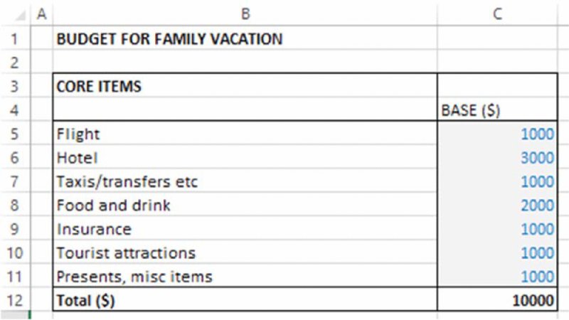
Figure 12.1 Base Cost Model
For the purposes here, we do not make any genuine attempt to capture the real nature of the uncertainty distribution for each item (as discussed in Chapter 9). We also make the (not-insignificant) assumption that the line items in the model correspond to the drivers of risk (see Chapter 7). This is in order to retain the focus on the core aspects relevant for this chapter.
In particular, we shall assume that:
- Each item can take any (random) value within a uniform range (of equally likely values).
- There are some event risks that may occur with a given probability, having an impact (in terms of additional costs) when they do so. In this example, these risks are assumed to be associated with changes in the availability of flights or of hotels compared to the base plan. The event risks are shown separately to the base model (in the form of a small risk register). For consistency of presentation, we have adapted the original model to include these event risks, with their value being zero in the base case. The range of additional costs when an event occurs is assumed to be uniform (and, for the hotel, includes the possibility that it may be possible to find a slightly cheaper one, as the lower end of the range extends to negative values).
The file Ch12.CostEstimation.Basic.RiskRanges.xlsx contains the values used for the probabilities and ranges, as shown in Figure 12.2.
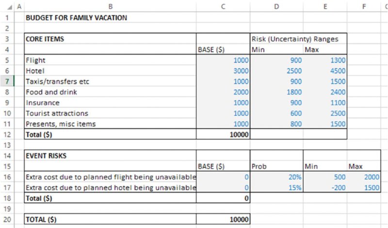
Figure 12.2 Cost Model with Values Defining the Uncertainty Ranges
12.2 Creating and Running a Simulation: Core Steps
This section describes the core steps required to create and run a simulation using Excel/VBA approaches, including the generation of basic random samples, the repeated calculation of the model and simple ways to store results. Later in the chapter, we discuss more general techniques that may be used in many real-life modelling situations in order to create more flexibility in some areas.
12.2.1 Using Random Values
The file Ch12.CostEstimationBasic.RiskRanges.WithRANDS.xlsx contains the next stage, in which the Excel RAND() function is used to generate uniformly distributed random numbers between zero and one; these are used to create random values within the uncertainty ranges:
-
For the uniform continuous ranges:

-
For the occurrence of the risk events:

The final impact of the event risks is calculated by multiplying the occurrence figure by the impact (so that the result will be a value of zero for the case of non-occurrence and equal to the impact in the case of occurrence), as shown in Figure 12.3.
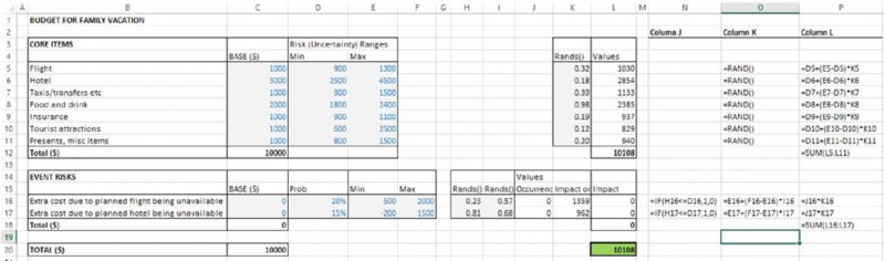
Figure 12.3 Cost Model with Uncertainty Distributions
This example is sufficiently simple that some important points about more general cases may be overlooked:
- For clarity of presentation of the core concept at this stage, the uncertain values generated are used as inputs to a repeated (parallel) model (i.e. that in column L, rather than in the original column C). Of course, most models are too complex to be built and maintained twice in this way: generally, the uncertain values would instead be integrated within the original model, for example by using an IF statement or a CHOOSE function to act as a switch that determines whether the input area to the original model (i.e. column C) would use the base values or uncertain values (so that the base values would need to be stored elsewhere and column C replaced with formulae).
- Where other distributions are required, as discussed in Chapter 10, the RAND() function would be used as an input into the calculation of the inverse cumulative distribution function.
12.2.2 Using a Macro to Perform Repeated Recalculations and Store the Results
With the model as built so far, the user can press the F9 key (which instructs Excel to recalculate), so that the RAND() functions will be resampled, and the model's values will update. In other words, each use of F9 will create a new scenario for the uncertain inputs and for the total cost. The automation of this step (so that it can be repeated many times) can be done using a looping procedure within a VBA macro.
The file Ch12.CostEstimation.Basic1.Macro.xlsm contains the VBA code (macros) for the simulation, so that the macros within it will need to be enabled.
(Alternatively, the file Ch12.CostEstimation.Basic.RiskRanges.xlsx may be used as a starting point for readers wishing to build the model from scratch by following the steps described below; in that case, the workbook would have to be resaved as a macro-enabled one, with the .xlsm extension, when using Excel 2007 onwards.)
12.2.3 Working with the VBE and Inserting a VBA Code Module
The Visual Basic Editor (VBE) can be accessed either using the Alt+F11 shortcut or (from Excel 2007 onwards) from the Developer tab. (The Developer tab is usually hidden by default and can be shown using the Excel Options, e.g. in Excel 2013 choosing Customize Ribbon under the [Excel] Options and checking the box for the Developer tab; the procedures for Excel 2007 and 2010 are similar but slightly different, but the reader should be able to find this without difficulty.)
Once in the VBE, one needs to insert a new module (Insert/Module) into the workbook (Project) that is being used (not into another workbook that also may be open); this operation is shown in Figure 12.4. A code window should also appear once the module is inserted; if not, View/Code can be used to display it.
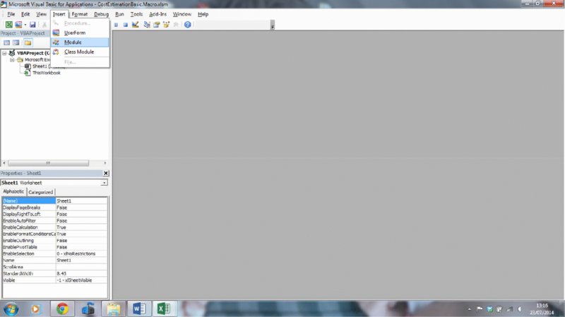
Figure 12.4 The Visual Basic Editor (VBE)
One can then start typing the macro (called a Sub, for subroutine) giving it an appropriate name, for example MRRunSim (spaces and words reserved by Excel/VBA are not allowed).
(The same basic procedure applies to user-defined functions, with the word Function used in place of Sub; functions also require a return statement. Section 12.5.3 provides more information.)
12.2.4 Automating Model Recalculation
The VBA statement Application.Calculate recalculates the model (Application refers to the Excel application). This is analogous to pressing F9 in Excel, and the required syntax could also be established by recording a macro during which one presses F9 (i.e. selecting Developer/Record Macro, pressing F9 and then using Developer/Stop Recording), and viewing the code that would have been inserted into a new module within the VBE.
At this stage the code would read:
Sub MRRunSim()
Application.Calculate
End Sub
It is often convenient to resize the VBE and Excel windows so that they are shown side by side, with each taking a half-screen. This will allow more transparent testing of the code by observing the worksheet updating as the code is run or tested.
Generally, rather than running the code all at once (see later), one may first run through it step by step using F8 repeatedly from within the VBE window (placing the cursor at the beginning of the Sub), as shown in Figure 12.5. The code line that is about to execute will be shaded yellow, and on execution those values that are affected by the RAND() functions will change.
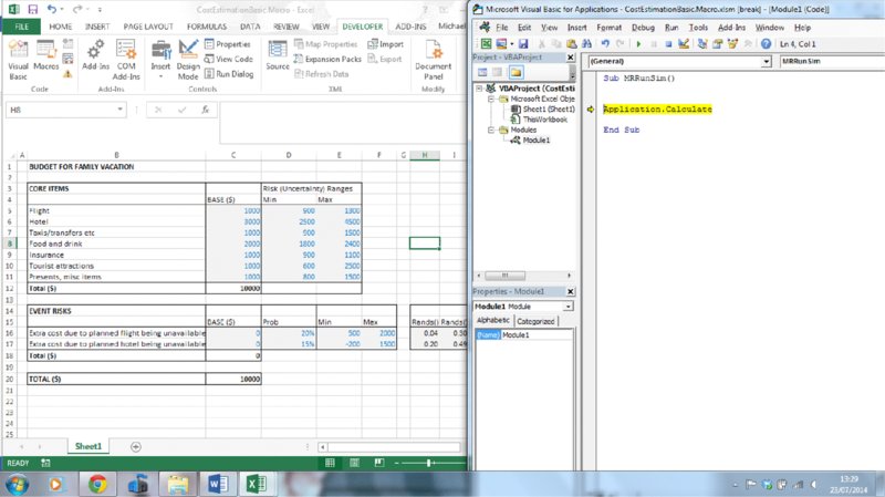
Figure 12.5 Split Screen of Uncertainty Model and VBE with Code Window
12.2.5 Creating a Loop to Recalculate Many Times
The next stage in the process would be to put the code within a loop, so that it could be run several times automatically. When initially developing and testing code, one would create a loop that would run only a few times (such as 10); once the code is working one would, of course, increase this (typically) to several thousand.
The core looping structure is a For loop (which is closed with the Next statement, so that the code knows to return to the beginning of the loop and increment the indexation number i by one):
Sub MRRunSim()
For i = 1 to 10
Application.Calculate
Next i
End Sub
Once again, one may step through the macro using F8 (one can escape from the step-through procedure using the Reset button [![]() ] in VBE, to avoid having to run all 10 loops if one feels that the code is working).
] in VBE, to avoid having to run all 10 loops if one feels that the code is working).
Of course, at this point, the model is recalculating new values at each pass through the loop, but the results are not yet being stored.
12.2.6 Adding Comments, Indentation and Line Breaks
As the code starts to become longer and a little more complex, one would ideally add comment lines to document what it is trying to achieve. A comment line is one that starts with an apostrophe and (automatically) appears in green text. It will not be executed when the code is run, but rather will be skipped over. For very simple code, comments may be regarded as unnecessary. However, it is usually preferable to create comments as the code is being written (and not afterwards), as it is otherwise easy to overlook the documentation of important items or the limitations of applicability of the code. Therefore, generally, comments should ideally be used even in simple situations, in order to avoid cases arising where code that has been gradually developed without comments becomes extremely complex to audit.
Another use of comment lines is to retain alternative functionality that can be flexibly used (i.e. turned on or off) without have to keep rewriting (and testing) the code: by simply adding or deleting an apostrophe before the relevant code, the line will be treated as a comment or as executable code respectively (this method is also useful when testing code).
Indenting the code lines can improve visual transparency. For example, the code within a For…Next loop can be indented. This can be done with the tab key (the tab width of indenting can be reduced from [the default of] four to one or two using VBE's Tools/Options menu); this is often preferable when multiple indentation is required (e.g. for loops within loops).
The use of “ _” (SPACE UNDERSCORE followed by pressing ENTER) continues the code on a new line, and will often help to make long lines of code easier to read.
(These techniques are used selectively in the files provided, although when showing code in the text we often delete the comments to aid the focus on the code lines.)
12.2.7 Defining Outputs, Storing Results, Named Ranges and Assignment Statements
Simulation outputs are simply those items that are to be recorded at each recalculation of the simulation so that they can be analysed later. As a minimum, this would include at least one traditional model output (i.e. the results of calculations) but generally may also include the values of some inputs or intermediate quantities, so that other forms of results analysis can be undertaken.
The most robust way to define outputs is to name the Excel cell containing that output. For example, the statement Range(“O20”) would always refer to cell O20, and thus may no longer refer to the desired output cell if a row were added in the Excel worksheet before the existing row 20 (which contains the output in the original model).
Similarly, if the results are to be stored directly into the model worksheet (as in our simple example), then it would also make sense to name not only the output cell(s) but also the beginning (or header) of the cell into which results are to be placed, so that this can act as a reference point for the storage operations, whose position would change by one row or column at each pass through the simulation loop.
Thus, generally, when using VBA, it is preferable to refer to Excel cells (or ranges) as named ranges, rather than cell references (using Formulas/NameManager). When doing so, it is often useful, more flexible and robust to ensure that the names have a workbook (not a sheet) scope, although some exceptions exist. This allows for the cell to be referred to in another worksheet (and from the VBA code) using its named range without having to change the code (for example, if part of the model were moved into another worksheet), and without requiring an explicit reference to a particular worksheet.
Of course, where named ranges are used in Excel, it is fundamental that they are spelt in the same way when used within the VBA code. In this respect, it can be helpful to use the F3 key in Excel to paste a list of the named ranges, and then to copy these into the VBA code when needed.
In our example:
- Cell L20 has been given the name SimOutput, which can be referred to within VBA as
Range(“SimOutput”).Value. - Cell O20 has been given the name NCalcs, so that
NCalcs=Range(“NCalcs”).Valuecan be used to define within Excel the number of recalculations, which is then read into VBA. Although the same name has been used for the Excel named range and the VBA code variable, their underlying definitions are different: one is a range in Excel and the other a VBA variable (one could give them different names if this were considered to be confusing).
There are also many options for where results data could be stored. Generally, it would normally be best to place them in a separate results worksheet, which will be done later in the chapter. For now, we use the simplest approach, which is to place them directly in the model worksheet, for example in some blank area underneath, or to the side of, the calculations. This is done:
- In Excel, by naming the cell L22 as SimResultsHeader.
- In VBA, by using the
offsetproperty of a range to ensure that the values of the simulation outputs are placed sequentially one row below the previous value when theForloop is executing (as theivalue is incrementing by 1 at each pass through the loop).
The code (excluding comments) at this point reads:
Sub MRRunSim()
NCalcs = Range(“NCalcs”).Value
For i = 1 To NCalcs
 Application.Calculate
 Range(“SimResultsHeader”).Offset(i, 0).Value = Range(“SimOutput”).
Value
Next i
End Sub
Note that the “=” sign is used to assign the value from the right-hand side to the left-hand side, i.e. it is an assignment operator, not a statement of equality. This can be confusing at first to some people, but in fact is the same as in Excel: one writes “=B2” in cell C2, in order to assign the value of cell B2 to the value in cell C2. Assignment statements will execute significantly more quickly than corresponding Copy/Paste operations (which initially may appear to be more intuitive); Copy/Paste procedures are not generally recommended, and are not used in this text.
12.2.8 Running the Simulation
One can step through the code (using F8 within VBE), and the results will start to appear in the model worksheet. Of course, in practice, one would generally wish to run the whole code once the testing phase is complete.
This can be done in several ways, although often the easiest route is to create a button (or other object in Excel) to which one assigns a macro. For example, one may insert a text box (Insert/Text/Text Box in Excel) and label it Run Simulation (for example) and then right click on the box to select Assign Macro from the drop-down menu; once the macro is assigned, clicking on the text box will run the macro. Alternatively, Form Controls can be inserted from the Developer tab using Insert/Form Controls, and the macro assigned to the inserted control (such as a button).
Other ways to run the code include:
- From within the VBE window, using F5 (the cursor can be placed anywhere in the subroutine when doing this).
- From Excel, using Alt+F8, or Macros/Run on the Developer tab.
As the code becomes larger, one may wish to run it to a certain point before stepping through line by line; this can be accomplished by using CTRL+F8 to run the code to the position of the cursor, from which point one can step through using F8. Alternatively, one can set a break point by clicking in the margin of the code and using F5 to run the code up until the break point, and step through using F8 afterward (one can click in the margin to remove the break point).
Figure 12.6 shows the results of running the simulation.
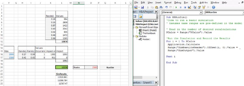
Figure 12.6 Basic Simulation Code and First Results
12.3 Basic Results Analysis
The file Ch12.CostEstimation.Basic1.Macro.xlsm contains the implementation up to this point in the text.
The file Ch12.CostEstimation.Basic2.Macro.xlsm contains the implementation of the additional features that will be discussed in the remainder of this section.
12.3.1 Building Key Statistical Measures and Graphs of the Results
In the simplest case, one may choose to build key statistical measures directly in the model worksheet. By using the value in the named cell NCalcs, the statistics functions can be given arguments that are dynamic and refer to the specific range in which the results data are contained (in this way, results of previous simulations do not need to be cleared). For example, one could find the average, the P90 and the frequency of simulated costs being lower than the base case with the formulae:
- =AVERAGE(OFFSET(SimResultsHeader,1,0,Ncalcs,1))
- =PERCENTILE.INC(OFFSET(SimResultsHeader,1,0,Ncalcs,1),9/10)
- =COUNTIFS(OFFSET(SimResultsHeader,1,0,Ncalcs,1),"<="&BaseCaseOutput)/Ncalcs)
(where, to create the last formula, the cell C20 was given the name BaseCaseOutput).
In this model, the average cost is around $12,000, the P90 is around $13,300 and the probability of costs being less than the original base figure is around 2%, as shown in Figure 12.7.
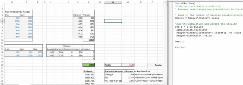
Figure 12.7 Basic Simulation Results and Statistics
One can also build graphs of distribution curves (although the Excel options to do so are generally significantly less flexible than those in @RISK, which are specifically designed for the purpose of displaying probabilistic data). To do so, one would need to define “bins” on the x-axis and count the number of outcomes within each one (using COUNTIFS or the FREQUENCY array function).
In the example file, we created 12 bins by dividing the x-axis into equally spaced regions between the lowest and highest values resulting during the simulation (calculated using the MIN and MAX functions). From these data, a line graph or a histogram is produced, as shown in Figure 12.8.

Figure 12.8 Basic Simulation Results, Statistics and Graph
Of course, in practice, one may wish to add more granularity (bins) to the x-axis, which can be done by adapting the bin range and formulae appropriately (this should be straightforward to implement for the interested reader). In addition, other preferred graph options can be applied to the generated data sets.
12.3.2 Clearing Previous Results
When running a new simulation it may be preferable to clear the previous results each time a new simulation is run (especially to cover the case where a new simulation has been run with fewer recalculations than the previous one, so that previous results do not get overwritten).
One can clear an Excel range (using VBA) by applying the ClearContents method. To automatically detect the range to be cleared, it is useful if the results range is not contiguous with any other range in the worksheet (apart from the title field SimResults); the CurrentRegion property of a range can be used to find the range consisting of all contiguous cells, which (once the header is excluded) defines the range to be cleared. The code would be:
With Range(“SimResultsHeader”)
NResRows = .CurrentRegion.Rows.Count
If NResRows > 1 Then
Range(.Offset(1, 0), .Offset(NResRows - 1, 0)).ClearContents
Else
'Do Nothing
End If
End With
Several points are worthy of note:
- The
With … End Withconstruct ensures that one uses the range SimResultsHeader as a reference point for all the operations contained within the construct. - The number of rows to be cleared depends on the number of data points in the current results range, not on the desired number of calculations (NCalcs) that is planned for the next run.
- The
If …Thenstatement ensures that the header text is not cleared: if there are no results currently stored then the number of rows in the current region of the header will be one (i.e. not greater than one) and so the code will move to theElseline (which results in no operations being performed). - If one were not aware of this syntax for the
CurrentRegionproperty of a range, one could record a macro whilst the Excel shortcut for the equivalent procedure was performed (i.e. CTRL+SHIFT+*). - As the code becomes more complex, one could think of dividing the current code for the
Subinto two separate subroutines: one to clear the contents and the other to run the simulation, and then to call each in turn from a master macro (this is done in some examples later in this chapter).
12.3.3 Modularising the Code
As code becomes larger, it is usually preferable to structure it in a modular fashion, in which tasks that are logically distinct are performed in separate subroutines, which are developed and tested separately. A master subroutine is then used to call individual procedures in the appropriate order. When doing so, one can use the Name box in the VBE Properties Window to name the modules to make it clear where modularised code is to be found, as shown in Figure 12.9. This is done in many of the examples later in the text.
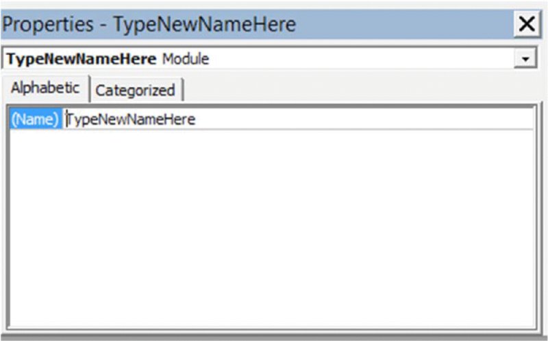
Figure 12.9 The VBE Properties Window
For some procedures contained in separate modules, one may wish to run them independently by creating a separate button in Excel for them. When the procedures are used from another procedure within the VBA code, one can use the Call statement to invoke this, as shown in the example file.
12.3.4 Timing and Progress Monitoring
The Timer function in VBA can be used in two places of the code in order to record the run time. For example, one could record the time using StartTime=Timer() toward the beginning of the code, and towards the end use EndTime=Timer(), so that the run time (in seconds) is the difference between these two. One can, of course, also use such techniques to measure the run time of only parts of the code. (These measures are, in fact, not very precise, in the sense that the simulation run time will depend on whether other applications are running in the background on the computer processor at the same time, but nevertheless often provide a useful general indication, especially if one is testing options that may have a major impact on the run time.)
At the completion of the simulation, one can display the total run time to Excel's StatusBar by inserting (toward the end of the code):
Application.StatusBar = “RunTime ” & Round(SimRunTime, 2) &
“Seconds ”
Similarly, the average number of recalculations per second could be calculated and displayed at the end of a simulation.
It can be useful to provide feedback during the course of a simulation as to the percentage completion, especially when using large numbers of recalculations (or where screen updating is switched off, as discussed below). This can be done by adding within the loop:
Application.StatusBar = Round((i / NCalcs) * 100) & “% Complete”12.4 Other Simple Features
Other simple features are possible to implement, and are briefly discussed in this section, although they are not implemented in the example files provided.
12.4.1 Taking Inputs from the User at Run Time
An alternative to using an Excel named cell to define the number of recalculations is to ask the user for this when the code is run. For example:
would create a variable NCalcs within the VBA code. The value of this would need to be placed in the model instead of any legacy value within the Excel range NCalcs, by using:
Range(NCalcs).Value = NCalcsThe latter feature of taking user input at run time is commented out in the example file, but may be implemented by deleting the apostrophes before the two appropriate code lines.
One may also allow the identification of the output cell to be set at run time (instead of having it as a predefined cell in Excel) by:
Set SimOutput = Application.InputBox(“Select Output Cell”, Type: = 8)The Set statement on the left-hand side is required to indicate that we are working with objects (cells) rather than simple values. The Type:=8 statement on the right-hand side defines that the nature of the input is a cell reference.
The taking of user input at run time may appear flexible, but has the disadvantage that often one wishes to be able to repeatedly run several simulations without changing any aspects of them (e.g. definitions of output cells, or number of recalculations); in such cases, it can be inconvenient to have to provide such input at each simulation run. Therefore, these approaches are not implemented in this text.
12.4.2 Storing Multiple Outputs
One may wish to analyse relationships between the values of variables in the model. For example, one may wish to create a scatter plot of the values and an input and an output, or of two outputs, or to calculate the correlation coefficient between an input and output or between an intermediate quantity and one of these, and so on. Of course, in such cases, one needs to store the data for each relevant variable, and then apply the required statistical or graphical process to these data.
In order to create the maximum flexibility in defining which items are to be stored during the simulation (which we shall refer to as outputs), it is often easiest to have a preset area designated as the output area (with the range given an appropriate name so that it can be referred to from VBA). In this way, the defining of a new output simply involves the creation of a formula reference from the cell in the output area to the cell in the model that contains the relevant calculation. Thus, if one needs to alter which output(s) are recorded, one can do this with a simple change of the cell being referred to, rather than having to rename the calculated cell.
This approach is used later in the chapter, and is combined with the placement of the output definition in a separate worksheet of the workbook.
12.5 Generalising the Core Capabilities
It is possible to generalise many of the aspects of the above approaches. The features discussed in this section are those that are implemented within the example files shown later, and so are not shown separately in their own files, despite their importance.
12.5.1 Using Selected VBA Best Practices
A number of other simple steps can be taken to enhance the transparency and robustness of the VBA code, especially as it becomes larger and contains more complex procedures or analyses.
- Requiring variable declaration. This can be done by placing the
Option Explicitstatement at the top of the code module, or under Tools/Options checking the Require Variable Declaration box. The main advantage of doing so is that one is alerted if a variable is used that has not been declared. In particular, typing errors in more complex code can be picked up (there may be many variables with fairly long but similar names, for example). In addition, it is computationally more efficient, as memory is allocated in advance of the variable being used. Declaration of a variable is done using theDimstatement, and key data types areInteger(values from − r15to 215 − 5, or to +32,767),Long(integers from − r63to 263 − 3) andDouble(any decimal values from approximately 10− 0pp to 10308).Rangemay also be required when a range variable is created. Examples of this are used in the subsequent models in this text. - Referring to ranges using full referencing, so that it is explicitly clear on which worksheet (and possibly which workbook) the ranges are to be found. This has not been implemented in the simple examples so far, but would be potentially important in more complex cases. In the examples in the text, the workbooks are all self-contained and generally use named ranges of workbook scope, and hence full referencing is generally not required in our particular examples.
12.5.2 Improving Speed
The issue of speed improvement in simulation models is generally complex and multifaceted. There are issues concerning individual process steps, such as the creation of samples of random numbers, the recalculation of the model, the processes to store results and processes to analyse results (such as sorting and binning processes, and statistical calculations), as well as issues of a more structural nature, such as the layout of the workbook.
Some core aspects of ensuring a reasonably efficient approach include:
- Using assignment statements, rather than Copy/Paste operations (as covered earlier).
- Declaring variables within the VBA code (as covered earlier).
-
Switching off the updating of the Excel screen when the simulation is running, and switching it back on at the end. To do this, one would place the following statements towards the beginning and end of the code (to ensure that, as a minimum, during the execution of the
Forloop, updating is switched off):Application.ScreenUpdating = False Application.ScreenUpdating = True - One could remove or switch off the use of the
Status Bardiscussed earlier to avoid any unnecessary calculations and communication overhead. - Separate the process of performing calculations on the results data from the simulation. For example, in the case of the model used so far, the results statistics functions are re-evaluated at each recalculation, whereas this is only needed once the simulation is complete. One could implement various approaches to ensure that such functions are not calculated at each recalculation of the simulation:
- Clear the formulae at the start of any simulation, and then reinstate them at the end (automatically). This is possible, but the syntax required to write formulae into Excel using VBA code can be complex (for example, within the COUNTIFS function, double quotation marks are required to avoid the single quotation mark around the “<=” from creating an error) and the array function for the frequency would be even more cumbersome.
- Place the results in a separate worksheet(s), which is referred to only when needed and whose recalculation is switched off during a simulation. This is the method that we shall use in the later examples.
- One may have to conduct a more thorough investigation of the time taken by different process stages and trying to find methods to improve the performance of each.
- In general, a major improvement in speed can be achieved by using VBA arrays to generate random numbers and store results as far as possible. Examples of this are given later in the chapter, but we do not pursue this here (despite its potential significance) in order to keep the focus on the main concepts, and to work first with simpler approaches that are initially easier to implement.
12.5.3 Creating User-Defined Functions
There is an important role for the use of user-defined functions when building simulation models in Excel/VBA. These include:
- To perform bespoke statistical calculations on a data set or on the output, such as calculating the semi-deviation of the output data (as described in Chapter 8).
- To calculate inverse (percentile) functions in order to sample from distributions (see Chapter 10).
- To create correlations between random samples (see Chapter 11).
As mentioned in Chapter 10, some readers may also wish to store their functions as a separate add-in, rather than in each individual workbook.
Examples of user-defined functions have been provided earlier in the text. For the purposes of completion of presentation, and for those using such functions for the first time, we note some core points:
- A function would be placed in a code module of the workbook, just like a subroutine.
- A function's name can be chosen from a wide set of possibilities, but there are some restricted words that are not allowed; largely the same principles apply as for subroutines.
- A function must have a return statement at the appropriate point (usually almost at the end), which defines its result to be shown to Excel.
- Functions can be entered in Excel either by direct typing or under the Insert/Function menu, where they are found within the user-defined function category.
- A function may need to be defined as
Volatileif it is required to be recalculated (at every Excel recalculation) even where its parameters are unchanged (as is the case with the Excel RAND() function, for example). Where necessary, this can be done by using theApplication.Volatilestatement at the beginning of a function; see elsewhere for examples. - Array functions can be created, and are entered as for other Excel array functions, i.e. by using CTRL+SHIFT+ENTER. The VBA code also generally needs to have an array to store these values; such arrays need to be declared (using the
Dimstatement), and are usually required to be resized at run time (usingReDim). An example that illustrates these points is the function to perform the Cholesky decomposition (Chapter 11).
12.6 Optimising Model Structure and Layout
Although there are many advantages to having most aspects of models in a single worksheet, there can be advantages to having multiple worksheets in some cases. In the context of a simulation model, it may be useful and most flexible to have specific functionality on separate worksheets:
- A “model” worksheet may contain (often ideally in a single worksheet) the main calculations (including inputs in many cases).
- A “simulation control” worksheet may contain a cell that defines the number of recalculations to run and a button to run the code, govern other user options, such as whether previous results are to be cleared or saved when a new simulation is run, and to aid navigation around the workbook, for example. (If such navigation tools are included, then it can be convenient for this worksheet to be automatically activated at the end of the simulation.)
- An “output links” worksheet that is used to link to the calculations in the model that are desired to be stored in a particular simulation run.
- A “results” worksheet that stores simulation results and may be either cleared out or overwritten as a new simulation is run, or new results may be inserted automatically at each run (with or without deletion of the older results).
- An “analysis” worksheet that links into the results sheets (as described later; this is done in such a way that the model becomes robust and flexible as results worksheets are deleted and added, by using indirect links rather than direct ones).
The file Ch12.CostEstimation.Basic3.Macro.xlsm uses this structure, and is described in more detail below.
12.6.1 Simulation Control Sheet
This contains the data on the number of recalculations that are desired to be run (the named range NCalcs was created having a global scope). It also contains buttons to run a simulation (which would automatically mean that a new results sheet is inserted), as well as a button to delete all existing results sheets. Note that we have given each worksheet a name using the Properties box within the VBE window, and these are the names that are used in the code.
There are also some buttons to aid navigation around the workbook, such as going to the model or analysis worksheets, for example:
Sub MRGoToModel()
With ThisWorkbook
 ModelSheet.Activate
End With
End Sub
Within the code modules, there is also a procedure to return one to this simulation control sheet; this is run automatically at the end of the simulation.
Sub MRGoToSimControl()
With ThisWorkbook
 SimControlSheet.Activate
End With
End Sub
12.6.2 Output Links Sheet
The use of a separate worksheet to link to the items calculated in the model creates a high degree of flexibility to change the outputs that are being stored during a simulation run. For example, one may wish to add new outputs, or decide that some previously captured outputs are no longer necessary.
In the example file, cell A1 of the corresponding worksheet has been given the Excel named range OutputHeaderStart. The user should type the name of the outputs along the first row (in a contiguous range), and place the cell links to the model in the second row, as shown in Figure 12.10.
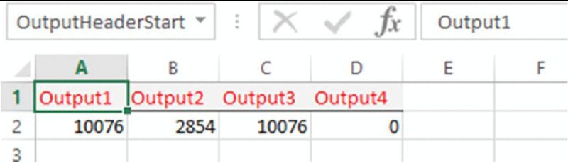
Figure 12.10 Use of Separate Worksheet to Reference Output Cells
Although only the first cell of the header range is defined, as the number of outputs may change, one can refer to the full header range (in this case A1:D1) using:
Set outrngHeader = Range(“OutputHeaderStart”).CurrentRegion.Rows(1)The right-hand side returns the first row of the current region of cell A1 (i.e. cells A1:D1 in this case) and assigns this to the variable outrngHeader. Therefore, if more outputs are added, this range will adjust automatically.
The Set statement is required as the variables concerned are both objects (i.e. ranges in this case) rather than values.
12.6.3 Results Sheets
In general, it would be most flexible and robust for the simulation results to be placed in a new worksheet, rather than in the model worksheet. Although one could work with a single predefined results worksheet, it is usually more convenient to have several possible ones, which are automatically inserted each time a simulation is run. Of course, after several simulation runs, one may wish to manually delete those that are not needed any more. However, in general, it can be convenient to have a mechanism to automatically delete them all on request.
The automatic insertion of results worksheets at each simulation run is easy to perform; the deletion of worksheets is also straightforward, providing one has a mechanism to distinguish those that are desired not to be deleted from those that are.
In the following code example, we automatically name the results worksheets as Results1, Results2, Results3, and so on. At the start of a simulation, the code counts the number of such worksheets in the workbook, and then adds a new one to the workbook, including the appropriate number in its name, i.e. if the workbook already contains Results1 and Results2, then the added worksheet will be Results3. (This part of the code would need to execute before the running of the simulation loop, so it can be placed either directly in the code or (as below) used as a separate subroutine that is called at that point.)
Note that the function loops through all worksheets (worksheet objects) in the workbook using the For Each … Next construct. The VBA Left function finds the first seven characters of the name, and these are converted to uppercase using the UCase function. If the resulting text equals “RESULTS” then the variable iCount is incremented by one, otherwise one moves to the next sheet.
Function MRCountResSheets()
Dim wksSheet As Worksheet
Dim iCount As Integer
iCount = 0
With ThisWorkbook
 For Each wksht In Worksheets
  If UCase(Left(wksht.Name, 7)) = “RESULTS” Then
  iCount = iCount + 1
  Else
  'Do nothing
  End If
 Next wksht
End With
MRCountResSheets = iCount
End Function
The code to add the sheet is then:
With ThisWorkbook
 isheetCount = MRCountResSheets  ' count number of results
sheets in model
 isheetNo = isheetCount + 1 'number of sheet to be inserted
 .Worksheets.Add.Name = "Results" & isheetNo ' insert sheet
End With
The code to run the simulation must, of course, write the data from row 2 of the output links worksheet into the newly created results worksheet (at each recalculation). The results data are written into the sequential rows of the results sheet (starting at row 2), and finally the output header names are placed in row 1 of the results sheet:
'Define output ranges and where results are to be written to
Set outrngHeader = Range(“OutputHeaderStart”).CurrentRegion.Rows(1)
icolcount = outrngHeader.Columns.Count
Set outrng = outrngHeader.Offset(1, 0) 'range of actual output
values
Set resrng1 = Worksheets(“Results” & isheetNo).Range(“A1”)
With resrng1
 Set resrng2 = Range(.Offset(0, 0), .Offset(0, icolcount - 1))
End With
'Run the Simulation and Record the Results to the new sheet
NCalcs = Range(“NCalcs”)
For i = 1 To NCalcs
 Application.Calculate
 resrng2.Offset(i, 0).Value = outrng.Value
Next i
'Place headers
resrng2.Value = outrngHeader.Value
One will generally wish to have code that deletes all the results worksheets at the click of a button. In a similar way to earlier, the following code uses a For Each … Next construct to loop through all worksheets in a workbook and delete those that start with the word “RESULTS” when converted to uppercase.
Note also that the use of Application.DisplayAlerts=False in the early part of the code ensures that code execution is not halted; Excel's default would be to ask (and wait) for user input before deleting a worksheet; the code switches back the defaults after it is run, using the Application.DisplayAlerts=True statement:
Sub MRDeleteResultsSheets()
Dim ResSheet As Worksheet
Application.DisplayAlerts = False
For Each ResSheet In ActiveWorkbook.Worksheets
 If UCase(Left(ResSheet.Name, 7)) = “RESULTS” Then
  ResSheet.Delete
 Else
 ' Do nothing
 End If
Next ResSheet
Application.DisplayAlerts = True
End Sub
12.6.4 Use of Analysis Sheets
There are several advantages to the structuring of the analysis of results in a separate worksheet(s) to those containing the results data:
- It allows (as above) the deletion of results worksheets without deleting any of the formula required for the analysis.
- A single analysis worksheet with standardised analysis can be created, with the formulae built so that the results data referred to can be chosen by the user in a flexible manner, and without having to rebuild formula links. This is done by using an INDIRECT function (rather than [say] a CHOOSE function), so that there are no direct formulae links to the results worksheets (which can be inserted or deleted independently of the analysis worksheet).
- To speed up the simulation, one can switch off the calculation of the analysis worksheet so that the analysis is only done after the simulation is complete (when the analysis worksheet's calculation is switched back on), rather than being performed at each recalculation of the simulation. (Note that this will only be fully effective if other workbooks are closed when the simulation is run, or their recalculation is also switched off.) To switch the recalculation in the specific analysis worksheet on and off, one would include code such as the following (at the beginning and at the end of the simulation, respectively):
Sub MRSwitchOffCalcAnalysis()
With AnalysisSheet
.EnableCalculation = False
End With
End Sub
Sub MRSwitchOnCalcAnalysis()
With AnalysisSheet
.EnableCalculation = True
End With
End Sub
Figure 12.11 shows the Analysis worksheet in the example file, after a simulation has been run, with some core output statistics built in. The linkages to the particular results worksheet that one wishes to consider are established by typing the name of the desired results worksheet in cell C2. The statistics immediately underneath are established using the regular Excel functions (as well as the semi-deviation function mentioned earlier), with the range that the function refers to be adapted automatically using the indirect reference provided by the name of the results worksheet. For example, the range used within each function:
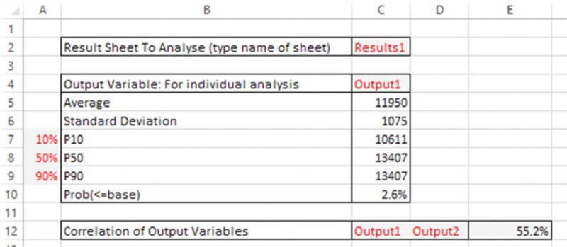
Figure 12.11 Use of Analysis Sheet that Links Indirectly to Results Sheets
This complex-looking formula simply states that the range is the one that is defined by referring to cell A1 of the worksheet specified in cell C2, and from that point, creating a range that starts one row below it (i.e. in row 2), but where the column position to start the range determined (using the MATCH function) as the column whose title (in row 1 of the results worksheet being referred to) matches the name of the output that one has entered in cell C4 of the analysis worksheet. From this starting point, a range of height NCalcs is created, and acts as the inputs to the functions.
(These formulae assume that each set of results has the same number of data points, equal to NCalcs; one could generalise the above, but the simulation code would also need to be adapted to record the value of NCalcs for each simulation within its own results worksheet.)
There are many further generalisations possible from this point:
- One could also generate a DataTable of results for a particular statistic. For example:
- One could create a one-way table that shows the average for all the outputs in a particular worksheet (this is done in a later example).
- One could create a one-way table that shows the correlation of each of many outputs with one single, particular output. If this latter output is a genuine model output (i.e. a calculated figure), whereas the others refer to the values of model input cells, then such figures can be used to produce basic correlation tables, as used in risk-tornado diagrams, for example.
- One could also generate graphs. However, chart data ranges in Excel do not permit the indirect form of reference used above (at the time of writing); therefore, chart data would generally have to refer directly to the results data. Alternatively, one could write a separate macro to retrieve the specific results data required and place this into a predefined column to which preset chart(s) may be linked.
Figure 12.12 shows a screen clip of the Analysis worksheet, showing two DataTables; the one shown in rows 14 to 18 is the correlation matrix between all outputs (calculated for the data from the Results1 worksheet defined in cell C2), and the one shown in rows 20 to 24 is the average value of several outputs for different simulation runs or results data sets.
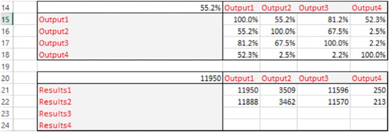
Figure 12.12 Additional Example of Output Analysis: Cross-Correlations of Outputs for a Selected Results Data Set, and Average Values for Each Output for Several Data Sets
12.6.5 Multiple Simulations
It can often be necessary to run a simulation if formulae in the model change, corrections are made, other outputs wish to be captured or if parameter values have been changed. In many such cases, there is no particular reason to need to compare the updated simulation results with those of prior simulations. However, in other circumstances, one may wish to be able to store and compare the results of one simulation run with those of another. For example, one may wish to see the effect of mitigation measures or of other decisions on a project, such as to judge whether to implement a risk-mitigation measure (at some cost) by comparing the results pre- and post-mitigation. More generally, the effect of other decisions may be captured in a model (such as the “decision risk” associated with whether internal management authorise a particular suggested technical solution, as discussed in Chapters 2 and 7), and one may wish to see the distribution of results depending on which decision is taken.
In principle, when using the above approach (in which a separate results worksheet is inserted automatically for each simulation), the running of multiple simulations poses no particular problem: one can simply change the model as required, rerun the simulation and compare the results, which will be recorded in separate worksheets.
One could also automate the process of changing the data in the model by embedding the basic simulation run within a second (outside) loop within the VBA code, so that a simulation is run at each pass through this outer loop. The index number of this loop (1 for the first simulation, 2 for the second, and so on) would then be assigned to the value of an Excel cell, and this cell would cause an Excel lookup function to return the required parameter values for that particular simulation run. For example, the outer simulation loop would be of the form For j = 1 to 5…Next j (where five simulations are to be run), and one would then name a cell in the Excel model (say) jIndex, so that, with the outer loop of the code, one includes a line such as:
Range(“jIndex”)=jso that the value of jIndex is changing for each simulation, and this value is used to determine the value of the model parameters for that simulation run (by using it as the argument of an Excel lookup function).
The file Ch12.CostEstimation.Basic4.Macro.xlsm contains an implementation of multiple simulations. The main adaptations to the previous example file are:
- Inclusion in the model worksheet of the data required for each simulation. In this case, we have assumed that we are testing the effect of the maximum values of all base items being different, using three possible values for each (of which the first is the original base case).
- Inclusion of a cell named jIndex in the model sheet, and the use of this cell to drive the CHOOSE function, which is then linked to the original values for the maximum of each variable.
- Inclusion of a cell named NSims in the simulation control worksheet.
- Addition of an outer loop to the VBA code.
Figure 12.13 shows the changes in the model worksheet, and the code shown below highlights the key changes to the VBA part.
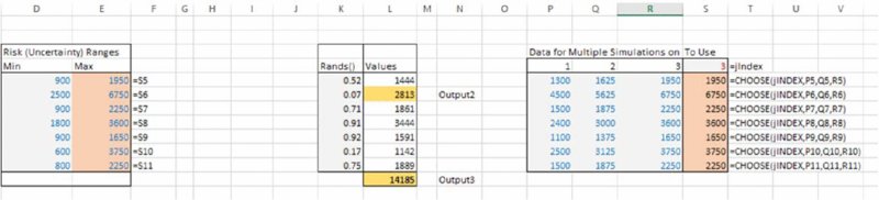
Figure 12.13 Adapted Model to Run Multiple Simulations in an Automated Sequence
Sub MRRunSim()
…
'Switch off calculation in analysis sheet
Call MRSwitchOffCalcAnalysis
NSims = Range(“NSims”)
For j = 1 To NSims
Range(“jIndex”) = j
  'Add a new results sheet
   AS PREVIOUS INCLUDING RUNNING SIMULATION AND WRITING RESULTS
TO RESULTS SHEET
Next j
'Switch on calculation in analysis sheet
Call MRSwitchOnCalcAnalysis
End Sub
In each of the above cases, one issue that may be of relevance (depending on the number of recalculations run and the accuracy requirements) is that one will not have control over the random numbers produced by the RAND() function; thus, some of the differences in the results of the various simulations will be driven by the different random numbers used in each, rather than by changes that occurred within the model. Overcoming this requires controlling the generation of random numbers, and is covered later in the chapter.
12.7 Bringing it All Together: Examples Using the Simulation Template
The mechanical techniques used so far in this chapter would, of course, in practice be combined with other tools discussed in this text, including the appropriate model design (Chapter 7), the use of distributions (Chapter 9), the creation of their samples (Chapter 10) and of correlations or dependencies between them (Chapter 11). This section presents some simple examples to show how this may be done in practice.
The file Ch12.TemplateExamplesMacro.xlsm contains various models that, for ease of presentation, are all contained in the single Models worksheet.
The template file has the following features:
- Its core structure and simulation component are based on the capability shown earlier in the chapter (except that we have not included the multiple simulation functionality).
- There are a number of distributions built in as user-defined functions:
- Bernoulli.
- Beta, beta general, PERT.
- Normal and lognormal (with both the natural and logarithmic parameters).
- Weibull, with both standard and percentile (alternative) parameter forms.
- The code to perform the Cholesky decomposition is included, as is the user-defined function mentioned in Chapter 11 (
MRMult), which performs the required matrix multiplication for both row and column vectors.
The five models that are included within the single Models worksheet (and whose outputs are captured in the OutputLinks worksheet) are each described below. Most of these issues should be self-explanatory for readers who have read the remainder of this text, so the descriptions are brief.
12.7.1 Model 1: Aggregation of a Risk Register using Bernoulli and PERT Distributions
Model 1 contains a typical risk register in which a risk occurrence is associated with an impact that is drawn from a PERT distribution, as shown in Figure 12.14.

Figure 12.14 Using the Simulation Template Model: Example 1
12.7.2 Model 2: Cost Estimation using Lognormal Distributions
Model 2 contains a cost estimation, in which the items are assumed to follow lognormal distributions, and is shown in Figure 12.15.
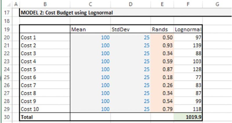
Figure 12.15 Using the Simulation Template Model: Example 2
12.7.3 Model 3: Cost Estimation using Weibull Percentile Parameters
Model 3 contains a cost estimation, in which the items are assumed to follow Weibull distributions, parameterised with their P10 and P90 values (as discussed in Chapter 9), and is shown in Figure 12.16.
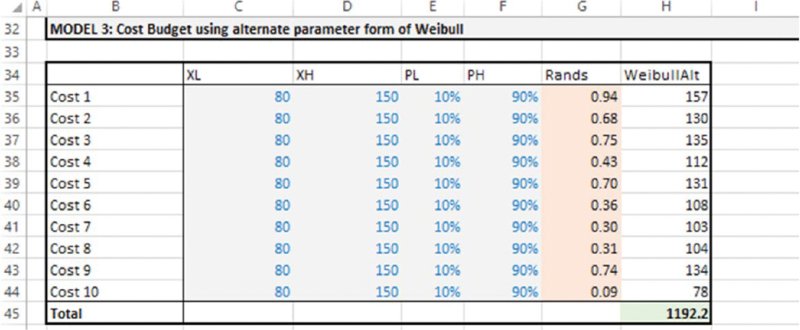
Figure 12.16 Using the Simulation Template Model: Example 3
12.7.4 Model 4: Cost Estimation using Correlated Distributions
Model 4 contains a cost estimation, in which the items are assumed to follow Weibull distributions parameterised with their P10 and P90 values (as in Model 3), in which these distributions are correlated using a correlation matrix that has been defined. The Cholesky matrix is produced using a user-defined function and multiplied by the array of random numbers (also the user-defined array function MRMULT that was discussed in Chapter 11) to create the final random samples, and is shown in Figure 12.17.
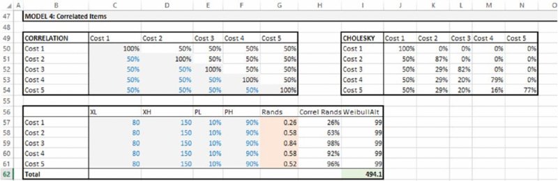
Figure 12.17 Using the Simulation Template Model: Example 4
12.7.5 Model 5: Valuing Operational Flexibility
Model 5 is similar to the model discussed in Chapter 4 to value operational flexibility (not in the presence of correlations). The price movement of each energy source is normally distributed. After the simulation is run, the relevant output results (in this case the average expenditure associated with each possibility using the values shown for Output5, Output6, Output7 and Output8 from the DataTable in the Analysis worksheet) are pasted into the appropriate area of the model (cells D68:D71) in order to calculate the value of the switching option. The model and option value (cell R71) are shown in Figure 12.18.
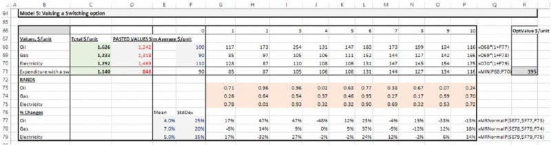
Figure 12.18 Using the Simulation Template Model: Example 5
12.8 Further Possible uses of VBA
The text so far within this chapter has focused on aspects of the use of Excel/VBA that are the easiest to implement within a simulation modelling context. Indeed – arguably with the exception of the Cholesky factorisation and the creation of correlated samples – all aspects covered so far have been relatively straightforward.
This section introduces some areas where one could develop the use of VBA further. Most of the topics relate to the use of the generation of random numbers within VBA, rather than directly in Excel. Once again, we aim to highlight those features of simulation modelling that can be fairly readily implemented in Excel/VBA without undue complexity, and without the requirement to have genuine application-programming skills.
12.8.1 Creating Percentile Parameters
In some cases it can be relatively straightforward to derive the parameters of a distribution given information about its percentiles; the Weibull distribution provides an example (as discussed in Chapter 9). However, in many cases, this is not easy or possible to do analytically (this applies both to distributions whose cumulative function has no closed-form solution, and to those where it has, but this function does not easily allow the derivation of the parameters in terms of percentiles, due to the specific nature of the formulae). In principle, one could always find the required parameters of a distribution from its percentiles by using iterative techniques. In particular, techniques such as Newton–Raphson iterations or Halley's method (see Chapter 11) could be implemented within many functions. These are usually highly effective as quantitative methods, as their precise implementation depends on the specific functions (so that few iterations are required to find the appropriate parameter values). On the other hand, such methods require a separate implementation within each function, which would be time-consuming to do for a wide set of functions.
12.8.2 Distribution Samples as User-Defined Functions
In the text so far, we generated random samples (for a probability value) in Excel using RAND(), and then used formulae for the inverse cumulative distribution to generate samples. One could consider an alternative in which the equivalent probability values are generated directly in VBA using the equivalent Rnd function. In such a case, the probability value would, of course, no longer be an input parameter to the function, for example code such as (where Prob is linked to the Excel cell containing the RAND() function):
Function MRWEIBULLP(alpha, beta, Prob)
MRWEIBULLP = beta * ((Log(1 / (1 - Prob))) ^ (1 / alpha))
End Function
would instead read:
Function MRWEIBULL(alpha, beta)
Application.Volatile
Prob=Rnd
MRWEIBULL = beta * ((Log(1 / (1 - Prob))) ^ (1 / alpha))
End Function
This approach would create a function that – when placed in an Excel cell – directly provided distribution samples (analogous to @RISK's distribution functions). However, it would not be a convenient approach if one desired to create a set of correlated random numbers (note that the correlation procedure we have implemented is one in which the probabilities are correlated, and so, by implication, the rank correlation of the samples has the same correlation coefficient, whereas in general the application of a Cholesky matrix after samples from the distributions have been created would not be a valid approach).
12.8.3 Probability Samples as User-Defined Array Functions
One possibility to be able to rapidly enter random numbers (to represent probability samples) in a multi-cell range is to use an array function.
The file Ch12.RandsinArray.VBA.xlsm contains the user-defined array function MRRandArray1(). The function has no arguments and can be used to simply select any (contiguous) range of cells in Excel and enter the function as an array function (i.e. using CTRL+SHIFT+ENTER). The function counts the number of rows and columns in the selected range and places a random number in each cell. Figure 12.19 shows an example of this being done in three cases: a column range, a row range and a range with multiple rows and columns:
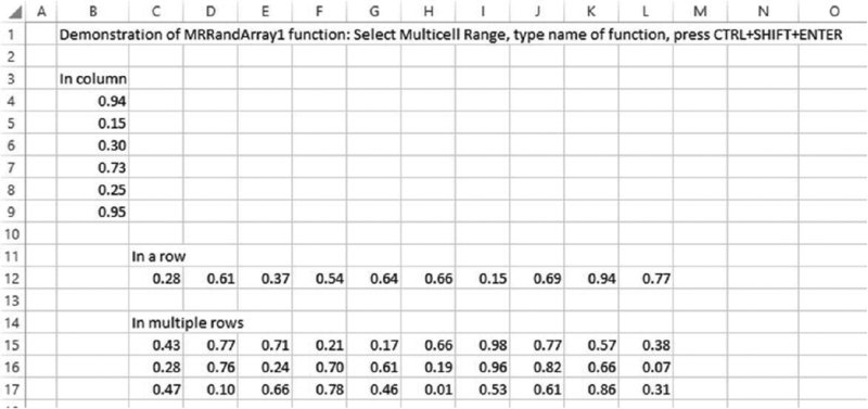
Figure 12.19 Creating a User-defined Array Function to Generate Random Numbers in Rows or Columns
Function MRRandArray1()
Application.Volatile
Dim Storage() As Double
NCols = Application.Caller.Columns.Count
NRows = Application.Caller.Rows.Count
ReDim Storage(1 To NRows, 1 To NCols)
For i = 1 To NRows
 For j = 1 To NCols
 Storage(i, j) = Rnd()
 Next j
Next i
MRRandArray1 = Storage
End Function
12.8.4 Correlated Probability Samples as User-Defined Array Functions
So far in this text, the Cholesky matrix that is required to create correlated probability samples has been placed explicitly in Excel, and the necessary matrix multiplication has also been performed in Excel. Since both steps can be written as user-defined functions, they could be combined (in various ways), in particular so that:
- The correlation matrix would be shown in Excel (but not the Cholesky matrix).
- The raw random number generation, the Cholesky factorisation and their final matrix multiplication would be conducted within the VBA code.
- A user-defined array function would be used in Excel to produce a set of correlated random numbers in either a single row or a single column range, based on the steps above.
- The function would use the correlation matrix as an optional argument: if no matrix was present, a set of random numbers could be placed in a range of any size (as in the above example), whereas if a correlation matrix was present, then the number of elements in the range would need to be the same as the number of variables (either rows or columns) in the correlation matrix.
The file Ch12.RandsinArray.DirectCorrel.xlsm contains the user-defined array function MRRandArray2(). The function has no required arguments; the correlation matrix is optional, a described above. Figure 12.20 shows a screen clip of the various possibilities, including its use in row and column form (of the appropriate size) when a correlation matrix is present, and in row and column form (of any size) when no correlation matrix is present.
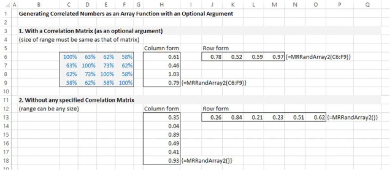
Figure 12.20 Creating a User-defined Array Function to Generate Correlated or Uncorrelated Samples in Rows or Columns
The code is shown below. The main function makes a separate call to a function MRRands, which produces a set of uncorrelated numbers, and is deemed Private so that it can only be accessed from this code module (and not from the Excel workbook, for example); this is done for reasons of robustness of use.
Note that, in practice, one may want to build in some error-checking procedures (for example, in terms of the size of the ranges, or whether the Cholesky procedure can be performed without producing an error, and so on). This is not done here in order to retain the focus on the core computational and algorithmic aspects.
Function MRRandArray2(Optional ByVal RCorrel As Range = Nothing)
Dim Storage1() As Double
Dim Storage2() As Double
Set wsf = Application.WorksheetFunction
With Application.Caller ' find size of input range
 NRangeTypeCols = .Columns.Count
 NRangeTypeRows = .Rows.Count
End With
If RCorrel Is Nothing Then
' no correlation matrix given; Generate random numbers only
  If NRangeTypeCols = 1 Then
   ReDim Storage1(1 To NRangeTypeRows)
   Storage1 = MRRands(NRangeTypeRows)
   MRRandArray2 = wsf.Transpose(Storage1)
  Else 'NRangeTypeRows = 1
   ReDim Storage1(1 To NRangeTypeCols)
   Storage1 = MRRands(NRangeTypeCols)
   MRRandArray2 = Storage1
 End If
 Exit Function
Else ' Do Cholesky factorisation and generate random numbers
  NCols = RCorrel.Columns.Count
   ReDim Storage1(1 To NCols)
   ReDim Storage2(1 To NCols, 1 To NCols)
   Storage1 = MRRands(NCols)
   Storage2 = MRCholesky(RCorrel)

   If NRangeTypeCols = 1 Then
     MRRandArray2 = wsf.MMult(Storage2, wsf.Transpose(Storage1))
    Else ' NRangeTypeRows = 1
     MRRandArray2 = wsf.Transpose(wsf.MMult(Storage2, wsf.Transpose
(Storage1)))
    End If
  End If
End Function
Private Function MRRands(ByVal NCols)
Application.Volatile
'Provides an array of random numbers
Dim Storage() As Double
ReDim Storage(1 To NCols)
 For i = 1 To NCols
 Storage(i) = Rnd()
 Next i
MRRands = Storage
End Function
12.8.5 Assigning Values from VBA into Excel
When creating random samples for probabilities within VBA, instead of linking these into the worksheet by using a function, one could instead assign values to the corresponding cells.
The file Ch12.RandsAssignedFromVBA.xlsm contains an example in which a macro is used to assign random numbers into a predefined range (given the name RangetoAssignRands in Excel, and shown as shaded in the screen clip in Figure 12.21). Once the macro is run (the button can be used), the range is filled with random values that are assigned from VBA, as shown in Figure 12.22. The code used is also shown.
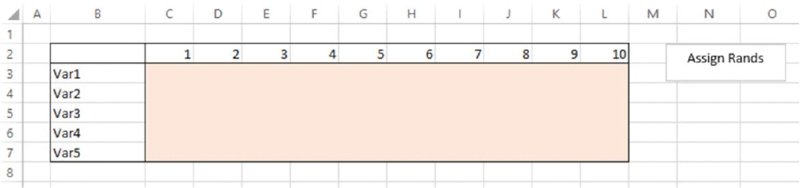
Figure 12.21 Named Range into Which Random Numbers are to be Assigned
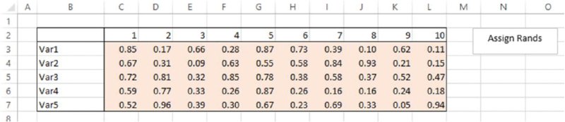
Figure 12.22 Completed Range after Assignment of Random Numbers
Sub MRAssignRandstoRange()
Dim Storage() As Double
With Range(“RangetoAssignRands”)
  NCols = .Columns.Count
  NRows = .Rows.Count
End With
ReDim Storage(1 To NRows, 1 To NCols)
For i = 1 To NRows
 For j = 1 To NCols
  Storage(i, j) = Rnd()
 Next j
Next i
Range(“RangetoAssignRands”).Value = Storage
End Sub
12.8.6 Controlling the Random Number Sequence
One can control the random seed that is used to generate the random numbers in VBA, so that the random number sequence could be repeated. This involves using Rnd with a negative argument (such as Rnd(-1)) to repeat the sequence followed by Randomize with a positive argument (such as Randomize(314159)), where a different value for the argument could be used to give a different, but repeatable, sequence.
The file Ch12.RandsinVBA.Seed.xlsm contains an example of this. It generates a set of random samples in VBA using a fixed seed that the user inputs into the model. For reasons of clarity and flexibility when the procedure is repeatedly used, any previously generated sequences are cleared, and the number of items to be generated is defined by the user within the Excel worksheet. (In practice, within a larger model and when using the multi-worksheet approach discussed earlier in the chapter, both of these user inputs would be placed on a worksheet that was dedicated to simulation control issues.) Figure 12.23 shows an example of running the procedure to generate 20 random numbers, using the fixed seed 314159. A reader working with the file can verify that the set of generated numbers is unchanged if the procedure is rerun at the same seed value.
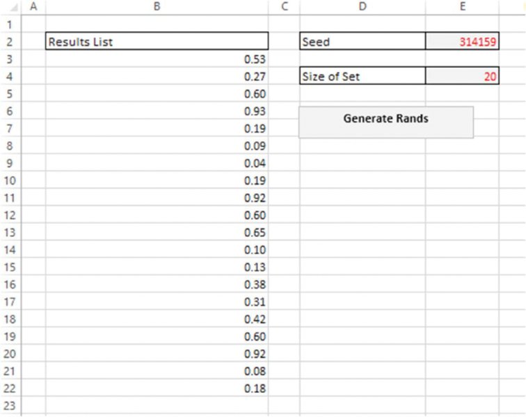
Figure 12.23 Generation of a Set of Random Numbers Using a Fixed Seed
The following is the code used within the file (including the subroutine call to clear out any previous numbers); it assumes that the required cells have been prenamed in Excel (which essentially should be self-explanatory here), i.e. SeedNo, NSizeofSet and RandsList, with the latter referring to the header cell of the range in which results are stored:
Sub MRGenRands()
Rnd (-1)
N = Range(“SeedNo”).Value
Randomize (N)
Call MRClearPreviousRands
With Range(“RandsList”)
 For i = 1 To Range(“NSizeofSet”)
 .Offset(i, 0) = Rnd()
 Next i
End With
End Sub

Sub MRClearPreviousRands()
With Range(“RandsList”)
 NRows = .CurrentRegion.Rows.Count
 If NRows <> 1 Then ' use this to avoid clearing out header when
data range is empty
  Set RngToClear = Range(.Offset(1, 0), .Offset(NRows - 1, 0))
  RngToClear.ClearContents
 Else ' Do Nothing
 End If
End With
End Sub
This procedure to generate a repeatable sequence of numbers could be combined with the earlier approach to generate numbers in VBA and then assign them into Excel. From a simulation perspective, one could generate all the required numbers before a simulation starts and assign (some of) them into the model at each recalculation of the simulation.
The file Ch12.RandsAssignedFromVBA.FixedSeed.xlsm contains an example of this, based on a generalisation of the earlier example. Figure 12.24 contains a screen clip in which the user fixes the seed and also defines the number of sequences required. In a simulation context, each sequence would correspond to a recalculation (iteration) of the simulation, so that one may set this figure to several thousand, for example; a reader working with the file will be able to do so, and to see that different sequences are generated. As mentioned earlier, one would also see that this method to generate the random numbers results in a simulation speed that would be significantly improved compared to the earlier methods.
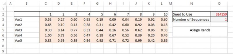
Figure 12.24 Generation of Sequences of Random Number Sets Using a Fixed Seed
The code used is as follows (once again, this assumes that the cells containing the seed and the number of sequences have been given predefined named ranges in Excel; and in practice these items may instead be placed within a separate worksheet dedicated to simulation control issues):
Sub MRGenRandsinArraySequence()
Dim Storage1() As Double
Dim Storage2() As Double
'Find size of array to generate, and create its storage space
 With Range(“RangetoAssignRands”)
   NCols = .Columns.Count
   NRows = .Rows.Count
 End With
 NSeq = Range(“NSequences”).Value

 ReDim Storage1(1 To NRows, 1 To NCols, 1 To NSeq)
 ReDim Storage2(1 To NRows, 1 To NCols)

'Fix the Seed, taking it from the sheet
Rnd (-1)
N = Range(“SeedNo”).Value
Randomize (N)

'Generate the numbers within the VBA array
For k = 1 To NSeq
 For i = 1 To NRows
  For j = 1 To NCols
    Storage1(i, j, k) = Rnd()
  Next j
 Next i
Next k

'Place Numbers sequentially in Excel i.e. as if doing a simulation
with repeated sets of rands
For k = 1 To NSeq ' This would be an outer simulation loop
 For i = 1 To NRows
  For j = 1 To NCols
    Storage2(i, j) = Storage1(i, j, k)
  Next j
 Next i
 Range(“RangetoAssignRands”).Value = Storage2
 'SIMULATION RECALCULATION WOULD GO IN HERE
Next k
End Sub
Note that:
- The code first generates all random numbers required in a three-dimensional array, before using only part of that array at each assignment to Excel, corresponding to a simulation recalculation (where the indexation number k defines the iteration [or recalculation] of the simulation loop).
- This procedure could also be generalised further by the inclusion of correlations between the random numbers. That is, given a correlation matrix defined within a model, its Cholesky decomposition would be performed purely in VBA and those factors used to create an array in VBA that creates correlated numbers. That is, in the above code, the array
Storage1would be combined with a Cholesky procedure to produce a new array of correlated numbers, which would then be those that are assigned into Excel at each simulation recalculation. The principles of doing so are a direct extension of the above approaches and so are not covered further here.
In terms of comparing speed of the various approaches, the following files each contain the same simple model, which generates the required probabilities in the corresponding ways:
- The file Ch12.TemplateForAssignmentComp.xlsm is based on generating the probabilities directly in Excel using the RAND() function.
- The file Ch12.RandsAssignedFromVBA.CompTemplate.xlsm uses the assignment method, in which all random numbers are generated within the VBA code and then used sequentially as the simulation is run. The code used has been adapted by using components from the above examples, and is not shown within the text to avoid repetition (the interested reader can inspect the code in the files directly).
Figure 12.25 shows the standard model used in each case. The model has been created in order that calculations within it represent the types of operations that generally occur in typical risk models, i.e. it uses distribution sampling, arithmetic operations and lookup functions. The probabilities generated are used to sample Weibull distributions using the percentile parameter form, the column sums are formed, the maximum value of these sums is determined and the position of this maximum within the range of sums is found. The simulation output is set to be equal to this maximum and its position.
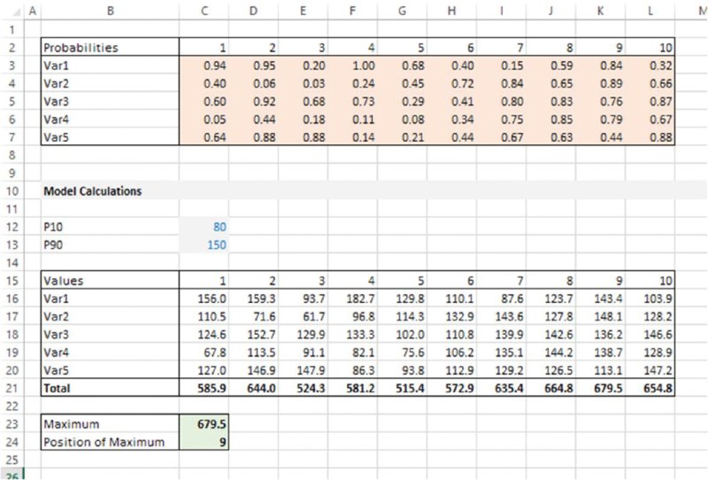
Figure 12.25 Model Used to Compare Speed of Assignment with Use of Functions
The reader may test the run speed of the two approaches (the run time is reported in each case at the end of the simulation); in the author's testing of these approaches, the assignment method runs approximately twice as fast as the within-worksheet generation method.
Note that in this comparison we have only altered the way that random numbers are generated; we did not alter the way that results are stored; in principle, the output calculations could be written (at each loop of the simulation) into a VBA array, with the results worksheet populated from this array at the end of the simulation run; interested readers can experiment with the effect of such issues on run time.
12.8.7 Sequencing and Freezing Distribution Samples
As mentioned in Chapter 7, when a simulation model requires a macro (or other procedure) to be run at each recalculation of a simulation, the input random numbers generally need to be “frozen” at each iteration; this is especially the case when using iterative procedures that themselves refer to values in the model (such as GoalSeek, Solver or the resolution of circular references), as such procedures may never converge if the values in the model are changing, as the procedure would generally cause the workbook to recalculate as the procedure iterated.
Thus, the approach of generating the probabilities within the worksheet would require an additional input range containing values that are assigned to each at each iteration/recalculation of the simulation, using a simple assignment statement. This is straightforward to do in principle. However, it would have the disadvantage that the ranges containing the RAND() functions were being resampled during such iterative procedures, even if such sampled values were not used in the calculations. This will slow down the calculation, and may create integrity problems in terms of knowing which input values actually created each output value.
Hence, the use of assignment statements using values generated from VBA code can be one way to implement the freezing procedure (i.e. no formal separate freezing procedure is necessary, rather at each recalculation of the simulation, the values created in VBA are assigned into the model, which is then recalculated and the additional procedure run, before proceeding to the next simulation step).
12.8.8 Practical Challenges in using Arrays and Assignment Operations
The generation of probability samples in VBA does have a number of advantages highlighted above, namely:
- Improved speed.
- Ability to control the random number sequencing, and hence to repeat a simulation exactly.
- Easier integration within the simulation loop of other procedures that require distribution samples to be frozen.
However, the main disadvantage of such methods in practice is where the set of probability values (i.e. the RAND() functions or assigned values) is not in contiguous ranges, and/or have different subsequent roles. For example, if some are required to be correlated together, and others are not, or separate random processes are calculated with probability values that are not in a single contiguous range (e.g. the occurrence and impact in the risk-register example), then such assignment approaches become harder to implement: one needs to develop a mechanism to count the number of random variables in the model (in order to size the VBA array), and also a mechanism to assign the values from the array to the relevant places in the model.
12.8.9 Bespoke Random Number Algorithms
To the extent that one decides to generate random numbers in VBA, one could also consider developing one's own algorithm to so do (such as using the well-known Mersenne Twister method in place of the VBA function Rnd()). Such endeavours are generally not trivial; of course, many such algorithms are available in @RISK, and so this is not discussed further here.
12.8.10 Other Aspects
Of course, with sufficient time, and the appropriate development of expertise, one could, in principle, develop the Excel/VBA application further, and eventually create a very wide range of functionality. Clearly, the more sophistication one develops, the more one may ask whether an equivalent functionality is already available in an add-in, and if so, whether the use of an add-in would be more time and cost effective. In particular, issues such as the speed of creation of a wide variety of quality graphical output, the use of a wide set of distributions (especially in the alternate parameter form) and a range of issues concerning simulation control represent significant advantages in the use of @RISK (others are mentioned in Chapter 13). In practice, perhaps after some initial exploratory activity has taken place using Excel/VBA approaches, it is often more effective to work with an add-in such as @RISK, especially in contexts in which quantitative risk assessment is aimed at achieving a wide organisational acceptance and implementation within standardised risk assessment processes.