
CHAPTER 13
Using @RISK for Simulation Modelling
This chapter covers the core aspects of using @RISK to design and build simulation models. We assume that the reader is a beginner with the software, and have designed this chapter so that it is self-contained from the point of view of the basic mechanics and features. However, the reading of this chapter alone would not be sufficient to build value-added risk models; the required concepts to do so are covered earlier in the text. The chapter aims to provide a basis to learn the core features of the software, rather than to cover the associated modelling and organisational alignment issues dealt with elsewhere. We do not aim to cover all aspects of the software; rather, we emphasise those topics that are required to work with the models in this text, as well as those features that are generally important from a modelling perspective. Thus, we do not cover the full set of graphics options, the detailed mechanics of formatting them, nor do we cover all of the results analysis possibilities, functions or other features; a reader wishing for more complete coverage can refer to the manual that is provided within the software, as well as to the Help features, other documentation and examples provided with the software (including its trial versions), and the Palisade website. As described at the beginning of the text (see Preface), readers who are working with a trial version of the software (which is time limited) may choose to skim-read this chapter (and the rest of the book) before downloading the software to work more specifically with some of the examples.
We start the chapter with a simple example that shows basic elements required to create and run a simulation using @RISK; the example is the same as that used in Chapter 12 for readers using Excel/VBA approaches. We then introduce some additional example models in order to show other key aspects of the software, many of which are used (or mentioned) in the examples earlier in the text. In the latter part of the chapter, we cover some additional features, including the use of VBA macros with @RISK.
13.1 Description of Example Model and Uncertainty Ranges
The file Ch13.CostEstimation.Basic.Core.xlsx contains the simple model that we will use as a starting point for the discussion. It aims to estimate the possible required budget for a family vacation. As shown in Figure 13.1, the initial model indicates a total estimated cost of $10,000.

Figure 13.1 Base Cost Model
For the purposes here, we do not make any genuine attempt to capture the real nature of the uncertainty distribution for each item (as discussed in Chapter 9). We also make the (not-insignificant) assumption that the line items correspond to the risk drivers (see Chapter 7). This is in order to retain the focus on the core aspects relevant for this chapter.
In particular, we shall assume that:
- Each item can take any (random) value within a uniform range (of equally likely values).
- There are some event risks that may occur with a given probability, each having an impact (in terms of additional costs) when it does so. In this example, these risks are assumed to be associated with changes in the availability of flights or of hotels compared to the base plan. The event risks are shown separately to the base model (in the form of a small risk register). For consistency of presentation, we have adapted the original model to include these event risks, with their value being zero in the base case. The range of additional costs when an event occurs is assumed to be uniform (and for the hotel, includes the possibility that it may be possible to find a slightly cheaper one, as the lower end of the range extends to negative values).
The (modified) file Ch13.CostEstimation.Basic.RiskRanges.xlsx shows the values used for the probabilities and ranges, as shown in Figure 13.2.
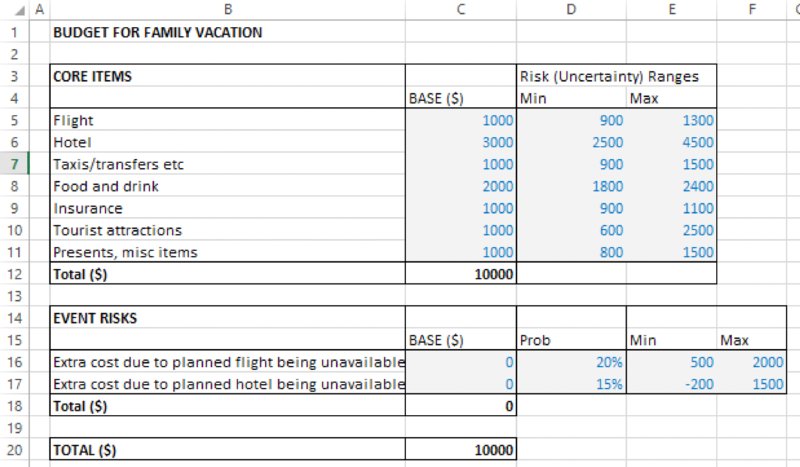
Figure 13.2 Cost Model with Values Defining the Uncertainty Ranges
13.2 Creating and Running a Simulation: Core Steps and Basic Icons
The screenshot in Figure 13.3 shows (part of) the @RISK toolbar (in version 6.3) that contains the key icons for getting started.
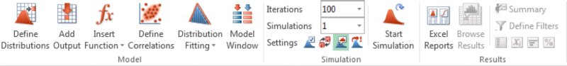
Figure 13.3 Core Icons to Build and Run a Simulation Model with @RISK
Recalling the discussion earlier in the text that the core of simulation is the repeated recalculation of a model as its inputs are simultaneously varied (by drawing random samples from probability distributions, which may also be correlated with each other), one can see the absolutely fundamental icons required for the purposes of getting started with @RISK (in the sense of implementing these core steps) are only a few:
- Define Distribution. This can be used to place a distribution in a cell (for transparency reasons, the parameters of the distributions would generally be cell references rather than hard-coded numbers).
- Add Output. This icon is used to define a cell (or a range of cells) as an output; such values are recorded at every iteration during the simulation, and are available for post-simulation analysis and graphical display.
- Insert Function. This @RISK icon can be used to enter distributions as well as statistics and other functions; such functions can also be entered using Excel's Insert Function icon (although one would then have to search for the applicable @RISK function category within the full function list). As in Excel, @RISK functions can also be entered by direct typing, but often the syntax is too complex for this to be practical except in special cases.
- Random/Static Recalculation. This icon (
 ) can be used to switch (toggle) the values shown in the distribution functions between fixed (static) values and random values. When random values are shown, the repeated pressing of F9 can be used to gain a crude idea of the range of values that would be produced during a simulation, and to test the model.
 - Iterations. In the terminology used in @RISK, an iteration represents a single sampling of all distributions in the model and a recalculation of the model, whereas a (single) simulation consists of conducting several (many) iterations (or recalculations).
- Start Simulation. This button will run the simulation with the chosen number of iterations.
- Browse Results. If a results graph does not appear automatically then one can use the Browse Results icon (which would usually appear as the default setting if the Automatically Show Results Graph toggle icon (
 ) is selected). The Tab key can be used to move between outputs if there are several.
13.2.1 Using Distributions to Create Random Samples
The file [email protected] contains a model in which we have used the Define Distribution icon to capture the uncertainty ranges both for the core cost items and for the impacts of the event risks (using the RiskUniform distribution), and the occurrence of the risk event uses the RiskBernoulli distribution (see Chapter 9 for a detailed discussion of the distributions). Note that one can use cell references as parameters of the distributions using the icon ![]() .The results of this process are shown in Figure 13.4.
.The results of this process are shown in Figure 13.4.
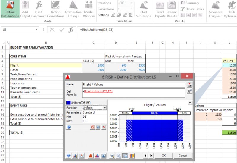
Figure 13.4 Cost Model with Uncertainty Distributions
This example is sufficiently simple that some important points about more general cases may be easy to overlook:
- For clarity of presentation of the core concept at this stage, the uncertain values generated are used as inputs to a repeated (parallel) model (i.e. that in column L, rather than in the original column C). Of course, most models are too complex to be built and maintained twice in this way: generally, the uncertain values would instead be integrated within the original model.
- When using @RISK to overwrite the value of an input cell in an existing model, several approaches are possible:
- Copying the original (base case) values to a separate range of the model, so that the values are shown explicitly, and replacing the contents of the original input cells with an IF statement (or, more generally, a CHOOSE function) driven by a model switch that directs the model's values (e.g. 1 = base case, 2 = risked values). This is the approach that the author generally prefers as it is often the most transparent, flexible and robust, and will often be used in many of the examples in the text (especially those where base cases are explicitly defined; in some cases, only the risk aspect is highlighted).
- Delete the cell contents before placing a distribution in it. This would not be ideal in general, as one would lose the original (or base case) value of the input.
- Insert the distribution directly in the cell (i.e. without first deleting the cell content). In this case (on the default settings), @RISK will automatically insert a RiskStatic function within the distribution function's argument list. For example, if this were done in cell C5, its content would then read =RiskUniform(D5,E5,RiskStatic(1000)). One can also insert a RiskStatic function (and link its value to a cell) into a distribution that initially does not contain one by using the Input Properties accessible using the icon
 , as shown in Figure 13.5. There are a number of advantages and disadvantages of this approach, but in general it is not an approach that we use in this text, which relies mostly on switches.
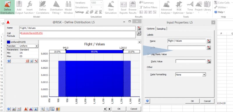
Figure 13.5 Defining Properties of an Input Distribution
13.2.2 Reviewing the Effect of Random Samples
When a distribution is placed in a cell, the value shown can be chosen to be either static or random. The choice can be set by using the Random/Static toggle ![]() . When using the static option, the values shown are either those defined through the RiskStatic argument (if it is present as an argument of the distribution) or as one of the options defined through the Simulation Settings icon (
. When using the static option, the values shown are either those defined through the RiskStatic argument (if it is present as an argument of the distribution) or as one of the options defined through the Simulation Settings icon (![]() ), and are discussed in more detail later. A simulation can be run even when the model is displayed in static view, as this is simply a viewing choice; when a simulation is run, random values are automatically used (by default).
), and are discussed in more detail later. A simulation can be run even when the model is displayed in static view, as this is simply a viewing choice; when a simulation is run, random values are automatically used (by default).
When the choice to display random values is made, one can repeatedly press F9 (to force Excel to recalculate), which will create new random samples. The use of this technique can be instructive to gain a crude idea of the range of values that would be produced during a simulation, and to test the model. Indeed, often when working with simulation models, it is better to work in this random mode, so that the model is reflecting the true random nature of the situation (on occasion, this may be confusing). For example, to compare the effect of structural changes in a model with a previous version, or for some other types of error diagnostic, one may wish to use the static view on a temporary basis.
Note that in the random view, the distribution functions directly provide random samples, rather than returning the cumulative probability or probability density values (as would be the case with Excel distribution functions and most other traditional statistical approaches to presenting distributions). Thus, the process of explicitly creating random samples by inversion of the cumulative distribution function (Chapter 10) is not necessary when using @RISK. Such an inversion process is generally used “behind the scenes” in @RISK, and is not explicit to the user.
13.2.3 Adding an Output
Once one has pressed F9 a few times (for example, to check that the calculations seem to be working), one would typically set the output(s) for the simulation. These are cells whose values will be recorded at each recalculation (iteration) of the simulation. The main purpose of setting an output is to ensure that the set of data is fully available for post-simulation analysis (such as the creation of graphs); the simulation statistics functions, such as RiskMean (see later), do not require their data source to be defined as an output.
In the example model, cell L20 has been set as an output by selecting the cell and using the Add Output icon, as shown in Figure 13.6. One can set the desired name of the output, or simply leave the software default names (in this latter case the RiskOutput() property function that appears in the cell will contain no explicit arguments; otherwise, its argument is a text field of the chosen name).
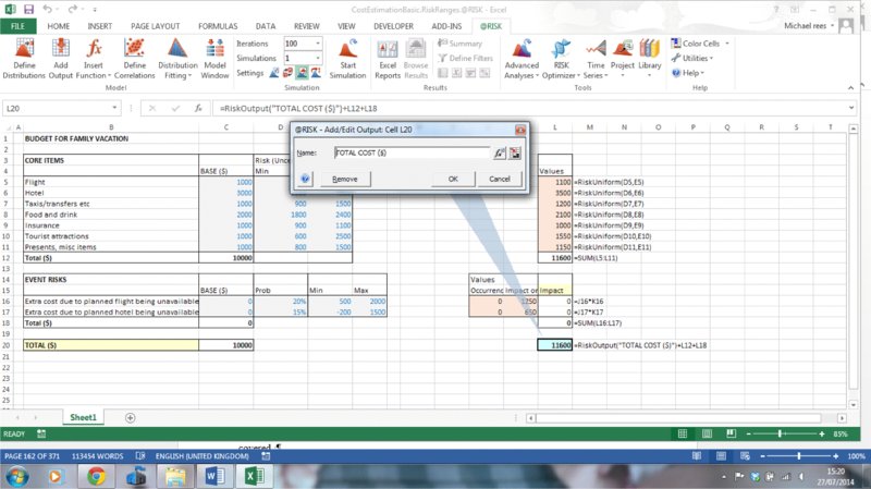
Figure 13.6 Adding an Output
13.2.4 Running the Simulation
One can run a simulation by simply pressing the Start Simulation icon. For the initial runs of a model (and when developing a large or complex model), one may choose to run only a small number of recalculations (which are called Iterations in @RISK), and to run more iterations once the model is closer to being finalised, or decisions are to be made with it. The drop-down menu can be used to set the number of iterations, or an alternative number (such as 2500) can be entered directly.
13.2.5 Viewing the Results
By default, @RISK has the Automatically Show Results Graph icon (![]() ) selected, so that a graph of the simulation output will be shown automatically (where there are several outputs, the Tab key can be used to move between them). If the icon is not selected, or a graph does not appear, then the Browse Results icon can be used (if no outputs are available to view, one may have forgotten to define any outputs!). The Tab key can be used to cycle through several output cells.
) selected, so that a graph of the simulation output will be shown automatically (where there are several outputs, the Tab key can be used to move between them). If the icon is not selected, or a graph does not appear, then the Browse Results icon can be used (if no outputs are available to view, one may have forgotten to define any outputs!). The Tab key can be used to cycle through several output cells.
Figure 13.7 shows the results of running 2500 iterations with the example model.
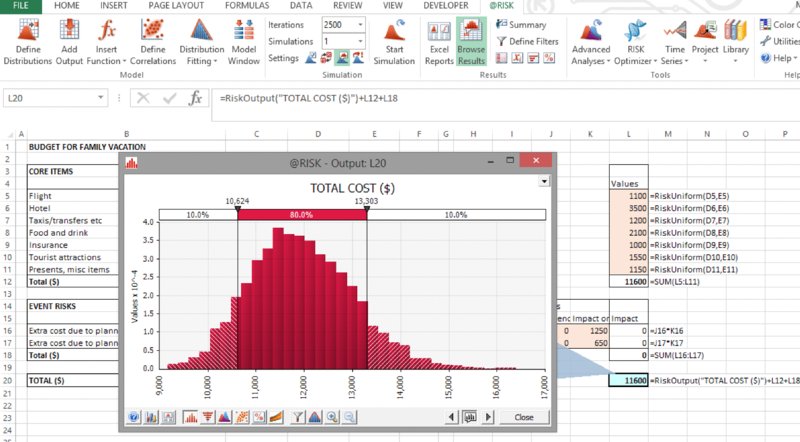
Figure 13.7 Simulated Distribution of Total Cost
As mentioned earlier in the text, the analysis of results would normally revolve around answering, in a statistical manner, the key questions that have been posed in relation to the situation, such as:
- What would the costs be in the worst 10% of cases, or the best 10% of cases?
- With what likelihood will the vacation cost less than or equal to the original plan?
- What would be the average cost?
Some of these answers can be seen from the graph (i.e. the P10 budget is about $10,600, and the P90 is about $13,300), whereas others would require additional information or displays:
- The delimiter lines on the graph can be moved to any desired place by selecting and moving them with the cursor; they provide information about the results distribution, without changing it. For example, one may wish to place the line at the base case value ($10,000) to see the probability of being below the base figure is about 2%.
- One could instead display the curve as a cumulative one instead of a density curve. This could be done by right-clicking on the graph and selecting Graph Options to bring up the corresponding dialog, or using the equivalent icon (
 ) directly on the graph.
 - One could add a legend of statistics to the graph, either by right-clicking on the graph and selecting Display (then selecting Legend) or by using the drop-down arrow at the top right of the graph (
 ) to choose Legend (with Statistics).
Figure 13.8 shows a cumulative ascending graph with a statistics legend and the delimiter line placed at the base case value.
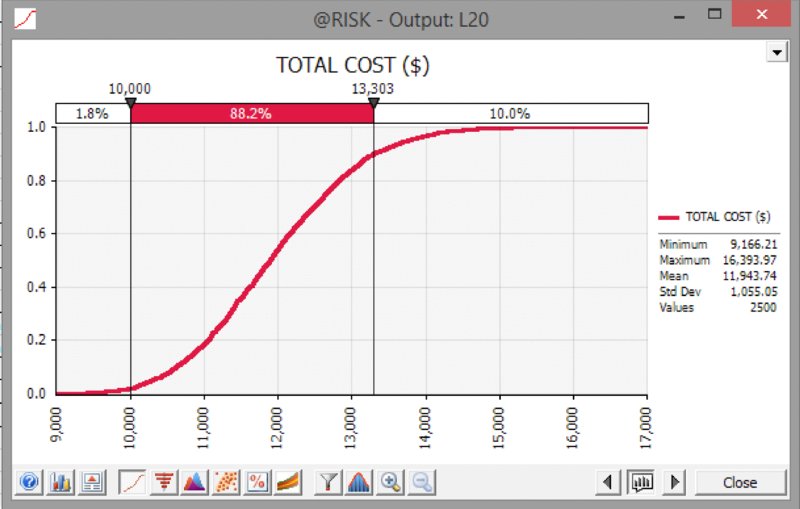
Figure 13.8 Cumulative Ascending Curve for Simulated Total Cost
The use of the Graph Options is fairly intuitive, and there are a number of tabs that can be used, for example to alter which statistics are shown in the legend, the colour of the graph, and so on. These are mostly very user-friendly and intuitive, and so although used at various points in the later text are generally not discussed in great detail here.
For readers who have worked through Chapter 12, one can note that the basic statistical results are similar (although not identical) to those shown in the Excel/VBA context. However, the overall visual interface, and the ease and speed of viewing and analysing inputs and results graphically is much quicker, richer and more flexible; this represents one key advantage of using @RISK.
13.2.6 Results Storage
There are a number of possibilities to store the results data that are, by default, presented when one first saves the model (the defaults can be changed under Utilities/Application Settings/General/Save Results). Possibilities include:
- Not saving the results (so that one would rerun a simulation the next time it was required).
- Saving the results within the workbook (the results data set is not visible, but is behind the scenes).
- Using an external (.rsk extension) data file that (apart from the extension) has the same name as the model's file, and is contained within the same folder.
- Within the @RISK Library. This feature is not covered within this text, as it is a separate database application using SQL Server, and although powerful, is beyond the scope of the modelling focus of this text.
For many day-to-day purposes, it is often simply easiest to save the results within the workbook. With large numbers of iterations, the amount of data saved can make the workbook file very large, in which case one of the other options may be considered. One can entirely clear saved results (in order to minimise the file size if e-mailing it, for example) under Utilities/Clear @RISK Data/Simulation Results.
13.2.7 Multiple Simulations
It can often be necessary to run a simulation if formulae in the model change, corrections are made, one wishes to capture other outputs or if parameter values have been changed. In many such cases, there is no particular reason to compare the updated simulation results with those of prior simulations. However, in other circumstances, one may wish to be able to store and compare the results of one simulation run with those of another. For example, one may wish to see the effect of mitigation measures or of other decisions on a project, such as to judge whether to implement a risk-mitigation measure (at some cost) by comparing the results pre- and post-mitigation. More generally, the effect of other decisions may be captured in a model (such as the “decision risk” associated with whether internal management authorise a particular suggested technical solution, as discussed in Chapters 2 and 7), and one may wish to see the distribution of results depending on which decision is taken.
In @RISK, one can run multiple simulations using the RiskSimtable function (each simulation uses the same number of iterations). The function requires a list of values as its arguments, and these are used in order within sequential simulations. Thus, the most flexible approach is usually to use the function with integer arguments (from one upwards); therefore, it simply shows the number of the particular simulation being run, and can act as an indexation number for an Excel lookup function that provides the actual parameter values for that particular simulation. When a simulation is not running, the RiskSimtable function returns the value of its first argument, so that for convenience it usually makes sense for the first element of a range whose values are looked up to be the base case (i.e. the values that one would most frequently desire to work with).
The file [email protected] contains an example of the implementation of this, in which the main adaptations required were:
- Inclusion in the model worksheet of the data required for each simulation. In this case, we have assumed that we are testing the effect of changing the maximum values of all base items, using three possible values for each (of which the first is the original base case).
- Inclusion of a cell containing the RiskSimtable in the model, and the use of this cell to drive the CHOOSE function, which is then linked to the original values for the maximum of each variable (the cell containing the RiskSimtable function has also been given the range name jIndex for consistency with the presentation in Chapter 12, although this is not necessary).
- Changing the number of simulations to three in the drop-down menu on the main @RISK toolbar.
Figure 13.9 shows the changes in the model sheet.
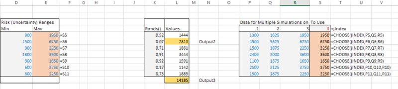
Figure 13.9 Adapted Model to Run Multiple Simulations in an Automated Sequence
By default, each simulation in @RISK will use the same set of random numbers, in order to ensure that differences in the results of the various simulations will be driven only by the changes that occurred within the model from one simulation to the next (one can alter the defaults for a particular model on Simulation Settings/Sampling and on the Multiple Simulation drop-down, selecting All Use Same Seed).
Figure 13.10 shows the results of running the model for the three simulations and using the overlay feature to overlay their results. (The overlay icon can be accessed by creating a graph of the simulation results as shown earlier, and then using the icon ![]() .)
.)
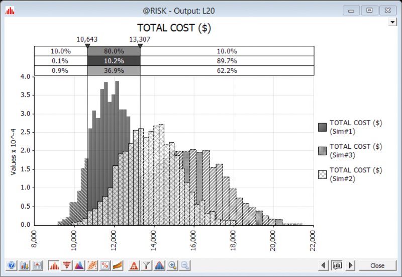
Figure 13.10 Overlaying the Results of Three Simulations
13.2.8 Results Statistics Functions
@RISK allows statistics of simulation results to be written directly into cells of Excel, using the @RISK Statistics functions (such as RiskMean); these can be accessed through @RISK's Insert Function icon, as shown in Figure 13.11.
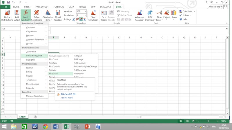
Figure 13.11 Use of @RISK's Insert Function Icon
Some key points relating to these functions are:
- The data source that each function requires is simply a reference to an Excel cell. This data source would often already have been defined as a simulation output. However, there is no requirement for this to be so in order for simulation statistics to be displayed, but the simulation must, of course, be run.
- There is some repetition between the functions. For example, RiskPtoX is the same as RiskPercentile, and RiskXtoP is the same as RiskTarget. In addition, functions with Q in place of P (such as RiskQtoX) work with descending percentiles (where P+Q=1).
- Each function has an optional parameter corresponding to the simulation number (where multiple simulations have been used):
- If the parameter is not included, the results of the first simulation are shown.
- If one uses the RiskSimtable feature in the way shown above (i.e. its arguments are the integers from one upwards that are placed in an Excel range), then the simulation number within a statistics function can be linked into the cells of that range (so that the statistics functions can more easily be copied to show the results of that statistic for each simulation).
The functions can also be accessed through Excel's Formula Bar using the Insert Function icon, and are contained within the category @RISK Statistics. Within this category one also finds the legacy RiskResultsGraph function, which pastes a graph of the simulation results into the workbook at the end of each simulation.
The statistic functions (most importantly RiskStdDev) do not include the correction term that is often needed in order for the statistics of a sample to provide a non-biased estimate. Thus, the functions effectively assume that the sample is the population, which, for large sample sizes (numbers of iterations), is generally an acceptable approximation (see Chapters 8 and 9).
By default, the functions calculate only at the end of a simulation; they can be set to recalculate at each iteration of a simulation under the options within Settings/Sampling, although this would rarely be required.
The function syntax can be confusing on occasion, because the “Data source” is a cell reference, but the statistics relate to the distribution of the value of that cell during a simulation. For example, if one were to use the RiskXtoP function to calculate the probability that the actual outcomes of a project were less than the base value, one may have a formula such as:
Such a formula would only be valid in a static (or base case) view; whilst the first function argument identifies a cell whose post-simulation distribution is to be queried, the second argument needs to refer to a fixed value. In addition, in the static (or base case) view, one may think that such a formula should evaluate to 0% (or perhaps 100%) but in fact (after a simulation and when in static view) it will show the frequency with which the calculation in the cell is below the value of that cell in the base case.
The file [email protected] has three statistics functions built in for each simulation. Figure 13.12 shows the results of these as well as the corresponding formulae.
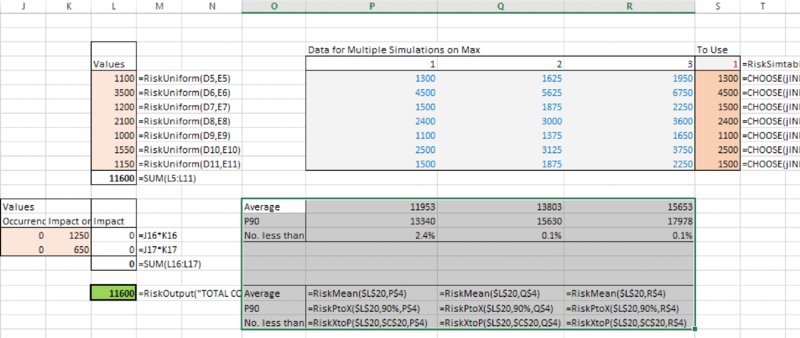
Figure 13.12 Use of RiskStatistics Functions with Multiple Simulations
13.3 Simulation Control: An Introduction
One of the important advantages of @RISK over Excel/VBA is the ability to easily control many aspects of the simulation and the model environment. The Simulation Settings (or Settings) icon (![]() ) provides an entry point into a set of features in this regard, some of which, such as the number of iterations or the number of simulations, are also displayed on the toolbar.
) provides an entry point into a set of features in this regard, some of which, such as the number of iterations or the number of simulations, are also displayed on the toolbar.
13.3.1 Simulation Settings: An Overview
When one has selected the Settings icon, a multi-tab dialog box will appear, as shown in Figure 13.13. Some of the points within this dialog are self-explanatory; for others, we provide a brief description either below or in later parts of the text.
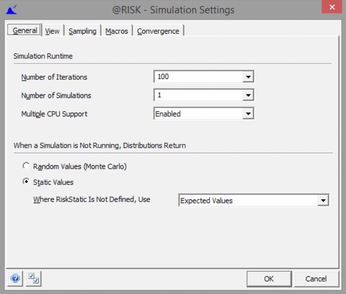
Figure 13.13 The Simulation Settings Dialog
13.3.2 Static View
Earlier in the chapter, we noted how a model using @RISK can be placed either in a random view or in a static view, by use of the toggle icon ![]() ; in random view one can press F9 to see resampled values. The use of this icon would be the same as switching between the options for Random Values and Static Values in the dialog below (Figure 13.13).
; in random view one can press F9 to see resampled values. The use of this icon would be the same as switching between the options for Random Values and Static Values in the dialog below (Figure 13.13).
We also noted that if a risk distribution contains the RiskStatic function as one of its arguments, then in the static view, the distribution will return the value shown by the argument of the RiskStatic function. For example, RiskTriang(D2,E2,F2,RiskStatic(B2)) would – when in the random view – create random samples from a triangular distribution (with minimum, most likely and maximum parameters equal to the values of the cells D2, E2 and F2), whereas in the static view it would show the value of B2. (Typically, B2 may be a base case value, for example.) The RiskStatic function will appear by default when one tries to place an @RISK distribution in a cell containing a number; this is both a protection mechanism to ensure that the number is not lost, and also a practical measure to allow (for example) a base case to be displayed.
However, in this text, we do not use the RiskStatic function in most of the examples provided. Instead, we prefer to use a switch in the model (generally an IF or CHOOSE function) to explicitly control whether the model uses random samples from distributions as its inputs, or uses the base case (or other fixed) values for the inputs. When this approach is used, if one selects the static view, then under Static Values, there are several options as to what a distribution may display (i.e. when the RiskStatic function is not present). These are available on the drop-down menu, and provide some additional viewing options that would not be present if the RiskStatic function were used:
- Mode. The modal value would often correspond to a base case.
- True Expected Values. Displaying average values is useful when all inputs are continuous distributions and the model is of a linear nature, as the calculations will then show the (theoretical) average of the calculations that would arise during the simulation.
- Percentiles. One could quickly see the effect of any systematic bias in the input assumptions, such as the effect of placing all inputs as their P30 values or their P70 values, for example.
- “Expected” Value. This is the default setting, and shows the value that is closest to the mean, but still valid. For continuous distributions, it will be the same as the mean; for discrete distributions it will be the closest valid outcome to the mean. The use of this as a default is a legacy feature, as in versions of @RISK prior to version 5 (i.e. approximately prior to late 2008), the other above options did not exist; arguably, a more appropriate default for later versions would be to use the modal values (if desired, this can be changed under Utilities/Application Settings/Default Simulation Settings).
The RiskStatic argument (if it is present) also governs the value that would be placed in a cell if the swap feature was used to swap out functions (Utilities/Swap Out Functions). If RiskStatic is not present, functions are swapped according to the setting within Utilities/Application Settings/Swap Functions. (Swapping could be used if the model were to be sent to someone who does not have @RISK; on the other hand, with the approach taken in most of this text [i.e. using a model switch], such swapping would not be necessary.)
13.3.3 Random Number Generator and Sampling Methods
As covered extensively in the text, in order to create samples of distributions (both in Excel/VBA and in @RISK) it is generally necessary to invert cumulative distribution functions, a process that requires random samples from a standard uniform continuous distribution. Thus, the quality of the samples generated ultimately depends on the quality of the methods to generate samples from a standard uniform continuous distribution. The generation of such numbers is not trivial; many algorithms have been developed by researchers in statistics (and related fields) that aim to generate “random” numbers. Such algorithms are (generally) fully deterministic, in the sense that once a starting point (or “seed”) is known, then other numbers in the sequence follow. One complexity in such algorithms is that the numbers generated should be truly representative of the process, but also not systematically biased. For example, if one is asked to choose five numbers that best represent a uniform continuous distribution between zero and one, possibly one would think of choosing 0.1, 0.3, 0.5, 0.7, 0.9; similarly for 10 numbers one might think of 0.05, 0.15, 0.25, …., 0.85, 0.95. We can see, however, that (the implied generalisation of) this algorithm is biased (and hence not truly representative), as certain parts of the range (for example, the number 0.43728) would only ever be chosen if the number of samples (iterations) used were very large. In addition to creating samples that are non-biased and representative, further criteria in the design of such algorithms are the cycle length before the numbers repeat (since a computer is a finite instrument, repetition will eventually happen in theory for any algorithm), as well as the computational speed.
Within @RISK, there are many possible ways to control the generation of random numbers (Simulation Settings/Sampling); these include the default Mersenne Twister algorithm (used from version 5) and the legacy RAN3I (used prior to version 5). The Mersenne Twister is widely regarded as being effective, and is essentially superior to the other algorithms within the software (at the time of writing); there is generally no reason to use any other generation method.
The software also contains two possible “sampling types”, known as Monte Carlo (MC) and Latin Hypercube (LH). The latter performs a “stratification” of the random numbers, so that they are equally distributed within each probability interval. Figure 13.14 shows a sample of 10 random numbers drawn from a uniform continuous distribution between zero and one, using both MC and LH sampling. One would generically expect to find one random sample in each interval of length 0.1, i.e. one number between 0 and 0.1, one between 0.1 and 0.2, and so on. One can see that with MC sampling, this is not necessarily the case: the numbers drawn for the 4th, 7th, 8th, 9th and 10th samples are in intervals in which a number already exists. In the LH approach, these samples have been replaced with different figures, ensuring that there is one sample in each (equal probability) interval.
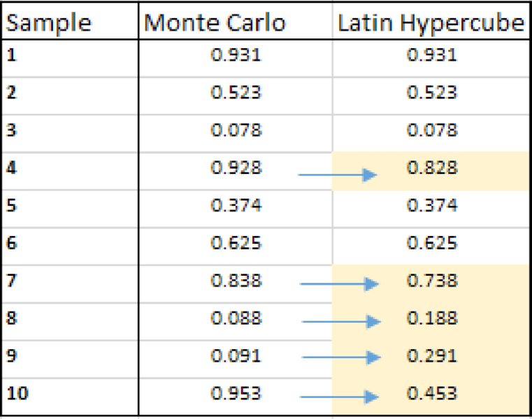
Figure 13.14 Adaptation of Random Numbers in Latin Hypercube Sampling
Generically, one may therefore consider LH to be a superior method. Unfortunately, the comparison is not as simple as one might wish to believe.
The general arguments used in favour of using LH are:
- It would require fewer iterations to achieve a given accuracy.
- It is worthwhile to spend a small amount of extra time to generate better random samples, because the time taken to generate random samples is a relatively small part of the overall time considerations. First, the time taken to run a simulation is a very small proportion of the total time taken to build, test and work with the model. Second, the computational time of running a simulation is also affected by the nature of the model and its recalculations, and by post-simulation data sorting and results processing. Especially if a model is large, but has only a few sources of risk, much time will be taken up by calculations, rather than sampling, so that for models with a large number of calculations (relative to the number of risk items), superior sampling methods should be preferred.
On the other hand, some key points that argue against LH are:
- The accuracy achieved after running a given number of iterations is not a relevant measure to compare the two methods; what is relevant is the total computational time (and perhaps also computer memory requirements). Measures of total computation time should include any set-up time after one initiates a simulation but before it actually starts to recalculate the model (this is often not included in some basic measures of simulation run time or simulation speed). These factors are harder for a user to estimate than simply comparing the number of iterations (although it is intuitively clear that, in order to perform stratification, LH sampling is more computationally and memory intensive than MC).
- In @RISK, LH performs the stratification only in a univariate sense, so that as soon as there are multiple risks, the effect of stratification starts to be lost: however, such multi-variation situations are precisely the situations when simulation modelling is most likely to be required. Thus, the benefits of LH are diluted in many real-life models.
One complexity in designing robust tests to compare the methods is that in most simulation models, one does not know what the exact value (or distribution) of the output is; this is usually why a simulation is being run in the first place!
However, a special case in which the correct value is known is when one uses simulation to estimate the value of π (3.14159…). An example is shown later in the text within the context of the @RISK Macro Language (XDK Developer Kit); these appear to show that LH is marginally preferable for models with small numbers of variables (say less than 10), beyond which there is little to choose between them.
13.3.4 Comparison of Excel and @RISK Samples
The existence of an effective random number generation method is one of the benefits of using @RISK in place of Excel/VBA. One can crudely compare the relative effectiveness of the random number methods using each approach by comparing the results of repeatedly sampling Excel's RAND() function with those of a RiskUniform distribution between zero and one. The effectiveness of such sampling is important, because in both Excel/VBA and @RISK, such samples are required to create (by inversion) samples of other distributions.
The file Ch13.RANDvsRiskUniform.xlsx contains an example in which this has been implemented; a sample of the results is shown in Figure 13.15 as a graphical overlay (after running a simulation of the model – each function is also defined as an @RISK output to aid in producing the overlay graphs); the @RISK settings are using Mersenne Twister generation and Latin Hypercube sampling (using a seed that was randomly chosen at run time). One can visually see the more even distribution of the numbers generated by @RISK.
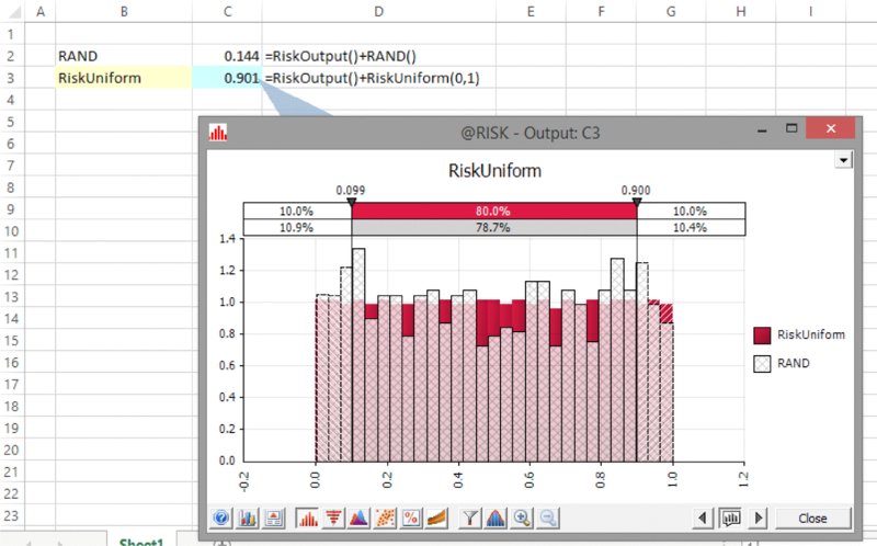
Figure 13.15 Overlay of Excel and @RISK Samples from a Standard Uniform Continuous Distribution
More formal methods to quantify the efficacy or random number generation methods are available but are generally highly mathematical and beyond the scope of this text.
13.3.5 Number of Iterations
Of course, all other things being equal, running more iterations will give a more accurate result. If one needs to justify or estimate the number of iterations required, one can use the Settings/Convergence options within @RISK, and set the number of iterations to Auto on the main toolbar.
13.3.6 Repeating a Simulation and Fixing the Seed
A simulation can be repeated exactly, if that is desired. One may wish to do this if results have not been saved or accidentally overwritten. In principle, the repetition of a simulation is a purely cosmetic exercise (for example, to avoid low-value-added discussions about why a P90 figure has changed very slightly, when that is only a result of statistical randomness, which may have no practical bearing on a decision, but can be inconvenient to have to deal with in a discussion with management!).
A simulation can be repeated if all of the following conditions hold:
- The sampling type and generator methods are the same.
- The number of iterations is the same.
- The seed used to run a simulation is the same. To repeat a simulation, the seed need not be fixed as such; rather, the seed of the previous simulation needs to be known and used again. However, in practice, it is often necessary to fix the seed at some preferred number and use this for all model runs. The seed can be fixed under Simulation Settings/Sampling.
- The model (and modelling environment) is the same. The notion of having the same model may seem obvious, but it is a subtle requirement in many ways, and really refers to the modelling environment as well as the model, for example:
- If the position of distributions were altered in a model (such as their rows being swapped), the model would have changed, as each distribution may use the random numbers that were previously used for others.
- If a distribution is added to a model, then the model has changed; even if the distribution is not linked to any formula in the model, the random number sequencing will be different.
- If another workbook containing @RISK is open when a simulation is run on a model, the results will generally be different than if this other workbook was closed. Even if this other workbook is not linked to the model in any calculatory sense, when they are both open, they will share the random number sequences used.
The data required for the repetition of a simulation (providing the model and its context do not change) are also contained as part of the information in a Quick Report that can be produced by clicking on the Edit and Export options icon (![]() ) of an output graph, or using the Excel Reports icon on the main toolbar.
) of an output graph, or using the Excel Reports icon on the main toolbar.
13.3.7 Simulation Speed
The speed of an @RISK simulation is largely determined by the computer used, and the structure, size and logic of the model. A number of simple ideas can be used to minimise the run time, but of course they typically will not have order of magnitude effects. These include (listed approximately in order of the easiest to the more complex to implement in general):
- Close workbooks that are not used in the simulation, as well as other applications.
- Within the Simulation Settings:
- Turn off the Update Windows (Display) and the Show Excel Recalculation options, and any other real-time (within simulation) update options, including convergence monitoring and the updating of statistics functions during a simulation (unless the intermediate values are required during a simulation, which is rare).
- Change the Collect Distributions Samples option to None; alternatively, mark specific inputs with the RiskCollect() function and change the setting to Inputs Marked with Collect, so that the input data for these samples will be available for tornado and related analyses.
- Remove unnecessary graphs, graphics and tables from the model, as these may take significant time to calculate and update, especially Excel DataTables. As mentioned in Chapter 7, an alternative is to place these items on a separate worksheet whose recalculation is switched off for the duration of the simulation and switched back on at the end (demonstrated in detail in Chapter 12).
- Work on items that generally improve the speed of single recalculation of a model. For example, ensure that any macros use assignment statements, rather than Copy/Paste, and that any lookup functions are appropriately chosen and most efficiently used, as well as considering whether circular references can be removed through model reformulation or simplification.
- Install both Excel and @RISK locally, instead of running over a network.
- Increase the system's physical (i.e. RAM) memory.
(Palisade's website and its associated resources [or its technical support function] may be able to provide more information when needed.)
13.4 Further Core Features
This section briefly describes further core features of @RISK. Many of them are used in the examples shown earlier in the text. Some of these features can also be implemented in Excel/VBA approaches, although doing so is often quite cumbersome and time-consuming.
13.4.1 Alternate Parameters
Most @RISK distributions can be used in the alternate parameter form; that is where some or all of the distribution parameters are percentiles of the distribution, rather than standard parameters. In Chapter 9, we discussed the benefits of doing so, and also provided some examples; readers are referred to that discussion for more information.
13.4.2 Input Statistics Functions
As well as providing statistics for simulation results, @RISK has in-built functions that provide the statistics of input distributions. Such functions return the “theoretical” values of their input distribution functions, as no simulation is required to calculate them. The parameters of the functions are analogous to those for outputs, except that the data source is a cell containing a distribution function (not an output calculation), and the name is appropriately altered, i.e. RiskTheoMean, RiskTheoStddev, RiskTheoPtoX, RiskTheoXtoP, and so on.
The functions are particularly powerful when used in conjunction with alternative parameter formulations, for example:
- One could use RiskTheoMax to find the maximum value of a bounded distribution that was created using the P90 figure in the alternate parameter form.
- One could use RiskTheoPtoX to find out the percentile values for distributions created with standard parameters, or RiskTheoMode to find the mode of such a distribution.
These techniques can be combined to approximate one distribution with another by matching percentile or other parameter figures, as shown in Chapter 9.
13.4.3 Creating Dependencies and Correlations
Earlier in the text, we discussed the topic of dependency modelling, including techniques to capture general dependencies (Chapter 7) and those between risk sources (Chapter 11); in this latter case, we noted that such dependencies are either of a parameter-dependent form (which is implemented through Excel formulae) or of a sampling form (which is implemented through the algorithms used to generate random numbers, and includes the generation of correlated samples or of those linked through copula functions).
In @RISK, the creation of correlated sampling is straightforward using the Define Correlations icon to create a correlation matrix in Excel, which is then populated with data or estimates. As mentioned in Chapter 11, the values used in this (final) matrix can also be taken from values calculated in other matrices (such as that which results from using the RiskCorrectCorrmat array function to modify any [original] inconsistent or invalid matrices).
In Chapter 11, we also mentioned that time series that are correlated only within periods can be created using this icon. Correlated series also often arise when explicitly using the Time Series features (such as Time Series/Fit), which are briefly mentioned later.
13.4.4 Scatter Plots and Tornado Graphs
One significant advantage of the use of @RISK over Excel/VBA is the ease and flexibility of creating visual displays of results data. Of course, when using such displays, it is important not to forget the key messages that such displays may show. As discussed in Chapter 7, in some cases one generally needs to design a model so that the appropriate graphs can be shown to decision-makers, and so that the model is correctly aligned with the general risk assessment process.
There is a large (an ever-increasing) set of graphical options within @RISK, so that it is beyond the scope of this text to cover these comprehensively. In this section, we briefly mention scatter plots and some aspects of tornado graphs, bearing in mind that some of the underlying concepts have been covered in Chapter 8, and some results using scatter plots have been presented at various other places in the text (Chapters 4 and 11). Those readers interested in a wider presentation of the options within @RISK can, of course, explore the possible displays by referring to the @RISK Help and other resources.
It is important to bear in mind that the relationships shown through a scatter plot also reflect the effect of dependency relationships. For example, if the X-variable of the scatter plot is highly related to other variables (such as positively correlated with them), then any change in an X-value will be associated with changes in the other variables, so that the Y-variable may change significantly, even if the apparent direct relationship between X and Y is not as strong.
By default, @RISK scatter plots show an output on the y-axis and an input on the x-axis. However, it is also often useful to show the values of outputs on each axis (for example, revenues and cost, where each is the result of several uncertain processes). In addition, one may also be interested in the equivalent display in which the X-values are those associated with some item that has not been originally included in the model (such as the total cost of hotels, i.e. that of the base uncertainty and the event risk together). One way to display such items is simply to create a new model cell containing this calculation, and to set this cell as a simulation output, so that its values are recorded and a scatter plot can be produced.
The file Ch13.MultiItem.Drivers.Tornado1.xlsx contains an example to illustrate some of the display options. The model is an extension of the one shown in Chapter 7 (containing common drivers of uncertainty), with the extension to create parameter dependencies (as discussed in Chapter 11); that is, the unit labour cost (cell G3) is an uncertain value that determines the most likely values for each of the other cost elements, which are themselves uncertain. The total project cost is the sum of these uncertain cost elements, but of course the unit labour cost is not contained within the calculation of the total cost.
Figure 13.16 contains a screen clip of the file, in which all uncertainties are modelled as PERT distributions.
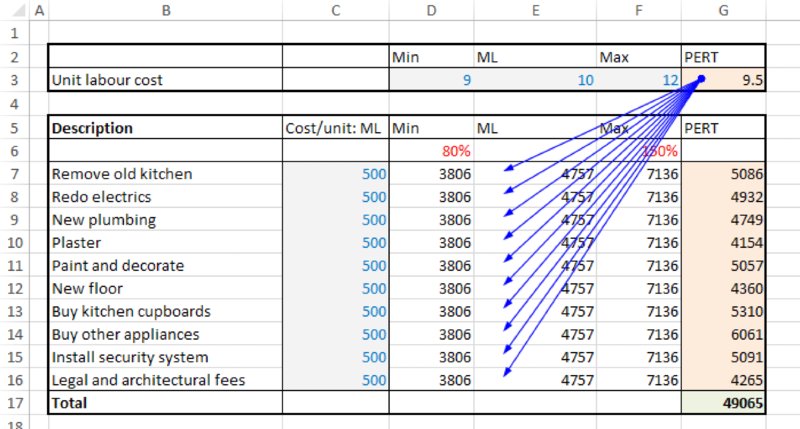
Figure 13.16 Cost Model with Common Driver of Most Likely Values for Each Uncertain Item
Following a simulation, one could produce a scatter plot of the output against any other cell (as long as this latter cell has been defined as an output, or is an input distribution, including those that may have been defined using the RiskMakeInput function; see later). Figure 13.17 shows a scatter plot of the total project cost against the unit labour cost.
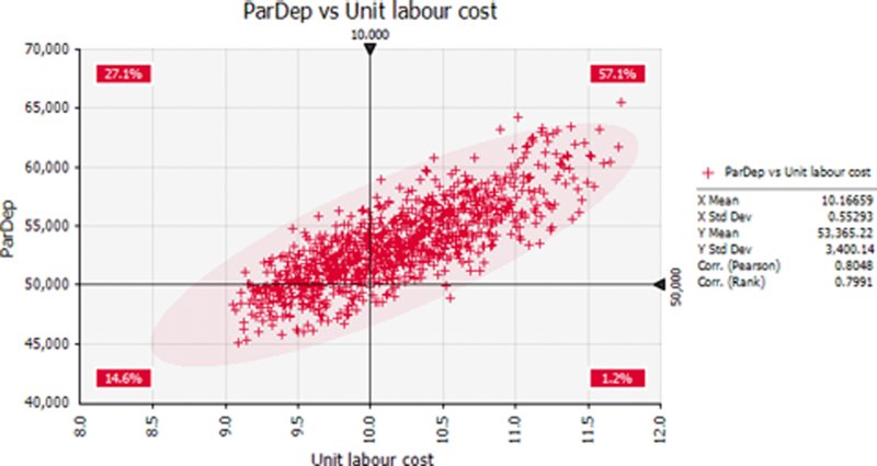
Figure 13.17 Scatter Plot of Total Cost Against Unit Labour Cost
One can see that there is a probability of around 80% that the project would cost more than the original base of $50,000; to see this, one can sum the two percentages that are above this point on this y-axis (as in Chapter 7, the base values are those when each input is set to its most likely value).
One can also see that there is an approximately 80% correlation between the items.
With regard to tornado charts, there are many possible variations of the displays of tornado graphs, which are briefly discussed below.
The classical tornado graph (i.e. those produced in the older versions of the software, such as prior to version 5, released in 2008) provided two main viewing possibilities:
- Correlation form.
- Regression form.
The correlation form shows the correlation coefficient between the selected output and the inputs. Some specific points are worth noting:
- The calculation of correlation coefficients usually requires large data sets in order to be very reliable (i.e. have a reasonably narrow confidence interval); small differences between coefficients are usually immaterial.
- As for scatter plots, such measures would, by default, implicitly include the effect of any dependency relationships in the model, and are valid measures when such dependencies exist.
These points can be illustrated with the same example as above. Figure 13.18 shows a tornado diagram of the correlation coefficients using the default settings (in @RISK 6.3, with Smart Sensitivity Analysis enabled) and running 1000 iterations. We see that the correlation coefficients are not all identical, even though every distribution has the same role and parameter values. (Note that the tornado bars can be given an appropriate name by using the Properties icon [![]() ] within the Define Distribution window to type the desired name [or take it from a cell reference], which results in the RiskName property function appearing with the main distribution function argument list.)
] within the Define Distribution window to type the desired name [or take it from a cell reference], which results in the RiskName property function appearing with the main distribution function argument list.)
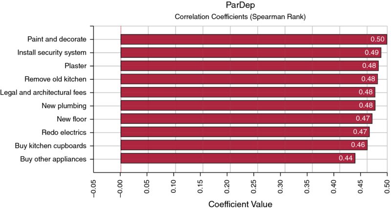
Figure 13.18 Tornado Chart of Correlation Coefficients with Smart Sensitivity Analysis Enabled (1000 Iterations)
A similar chart when 10,000 iterations are run is shown in Figure 13.19, showing that the coefficients are more nearly equal to each other in value.
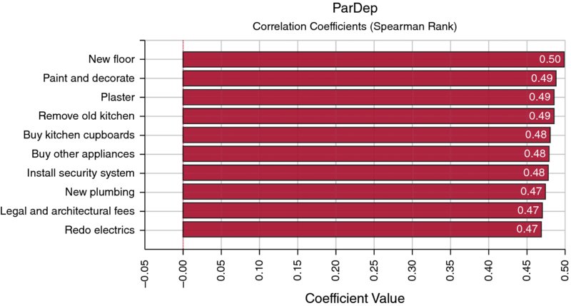
Figure 13.19 Tornado Chart of Correlation Coefficients with Smart Sensitivity Analysis Enabled (10,000 Iterations)
Note that the graphs do not show the unit labour cost as an item; this is because the default setting has screened out this item. By disabling the Smart Sensitivity Analysis (using the Sampling tab under Simulation Settings, for example), one can produce a chart as in Figure 13.20, in which this item is in first place. (A user deciding that the bar should not be shown after all can right click on the bar to hide it, and does not need to alter the setting and rerun the simulation.)
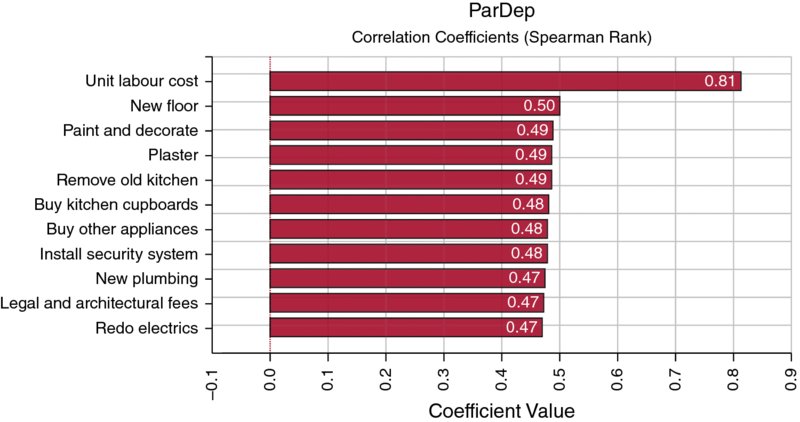
Figure 13.20 Tornado Chart of Correlation Coefficients with Smart Sensitivity Analysis Disabled
Note that in this model, the use of the Regression Coefficients option would produce a graph as in Figure 13.21. In other words, the coefficients are of equal size, but do not match the correlation coefficients. In addition, the unit labour cost item is excluded even though the Smart Sensitivity Analysis option was run on the disabled setting.
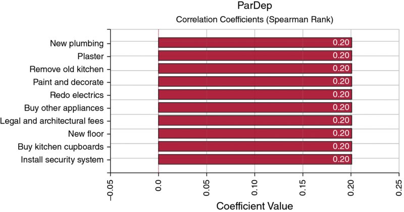
Figure 13.21 Tornado Chart of Regression Coefficients
We can recall from the discussion in Chapter 8 that the slope of a (traditional, least-squares) regression line that is derived from the data in a scatter plot is closely related to the correlation coefficient between the X- and Y-values, and to the standard deviations of each. However, such regression analyses are typically valid only when the inputs are independent, which in this case is not so.
The file Ch13.MultiItem.Drivers.Tornado2.xlsx contains an example in which the uncertain items are all independent. From Figure 13.22, one can see that the Regression Coefficients option in this case has coefficients that are similar to those that would be produced by the Correlation Coefficients option, which is shown in Figure 13.23.
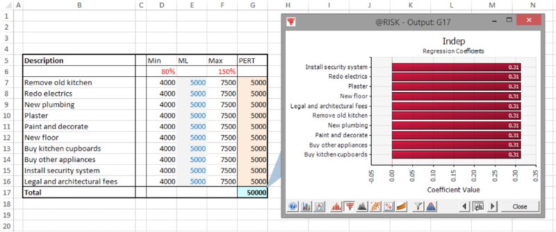
Figure 13.22 Tornado Chart of Regression Coefficients for Independent Items
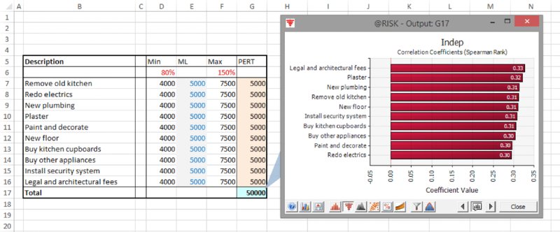
Figure 13.23 Tornado Chart of Correlation Coefficients for Independent Items
In cases where the items are independent, the sum of the squares of the regression coefficients will add to one, and hence these squared figures represent the contribution to the variance of the total output.
An option for the display of tornado graphs is the Regression-Mapped Values. As covered in Chapter 8, the slope of a regression line placed through a scatter plot is related to the correlation coefficient and the standard deviations of each:
Since the slope describes the amount by which the y-value would move if the x-value changed by one unit, it is clear that if the x-value is changed by σx then the y-value would change by an amount equal to ρxyσy. Thus, the mapped values can be directly derived from the regression coefficient values (i.e. the correlation coefficients that are derived through regression) by multiplying each by the output's standard deviation. Once again, such calculations only really make sense where the input distributions are independent of each other, because in the presence of dependencies, a movement of one variable would be associated with that of another, so the output would be affected by more than that implied through the change of a single variable only.
Another form of tornado graph is the Change in Output Mean. This is fundamentally different to the tornado graphs discussed above, as it is not based on correlation coefficients. Rather, the (conditional) mean value of the output is calculated for “low” values of an input and also for “high” values of an input. Figure 13.24 shows an example (using the model in which the items are independent).
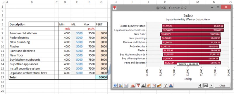
Figure 13.24 Use of Change in Output Mean Tornado Graphs: Independent Items
With respect to such charts, the following are worth noting:
- There is some statistical error in them, in the sense that the bars are not of identical size, even where the variables have identical roles and values.
- Dependencies between items will be reflected in the graphs. Figure 13.25 shows the equivalent chart for the model in which there is a common (partial) causality, as described earlier.
-
There is no clear directionality of the effect of an increase in the value of a variable (unlike for correlation-driven charts); see Figures 13.26 and 13.27.
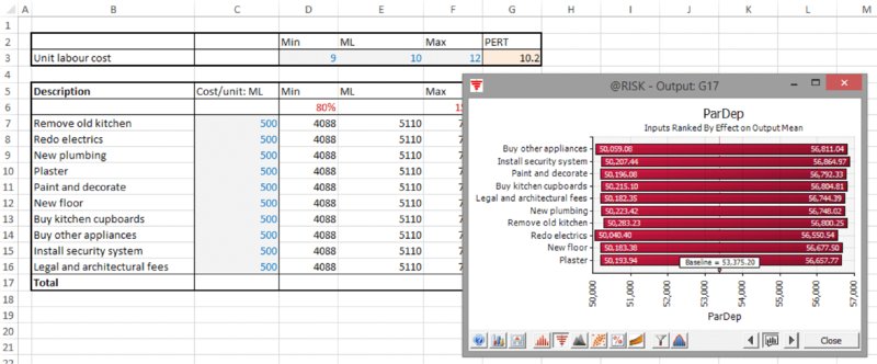
Figure 13.25 Use of Change in Output Mean Tornado Graphs: Items with Common Risk Driver
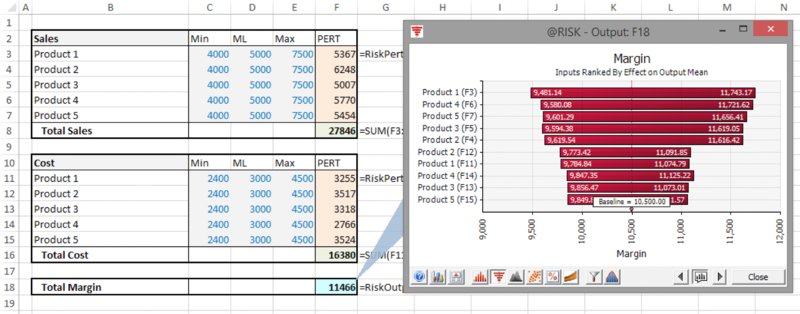
Figure 13.26 Use of Change in Output Mean Tornado Chart for a Model with Variables Acting in Positive and Negative Senses
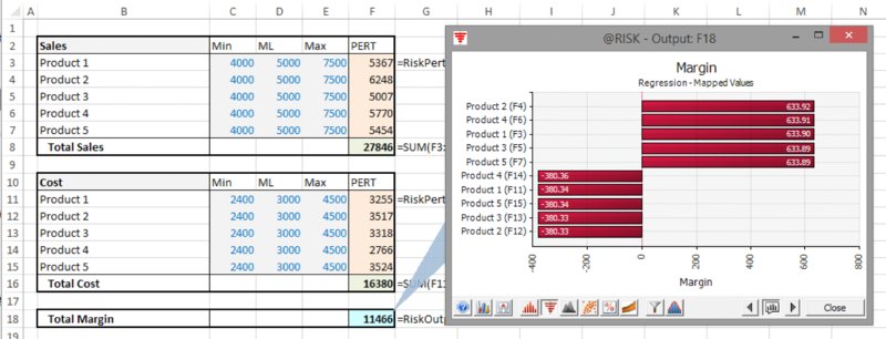
Figure 13.27 Use of Regression-Mapped Values Tornado Chart for a Model with Variables Acting in Positive and Negative Senses
The file Ch13.MultiItem.Drivers.Tornado3.xlsx contains an example in which the margin generated by a company is calculated as the difference between the total sales of five products and the cost of producing the products, on the assumption that all items are independent. Figure 13.26 shows the model using the Change in Output Mean tornado chart, and Figure 13.27 shows the Regression-Mapped Values one.
From the above discussion, and also relating this to the more general points made earlier in the text, a number of points are often worth bearing in mind when using tornado charts in practice:
- The charts show the effect of the variability of the uncertain items, whereas (as discussed in Chapter 7), in many cases, it is the effect of decisions that are often equally or more important from a decision-making perspective; thus, one should not overlook that “decision tornados” may need to be produced by a separate explicit process.
- In general, as there is a large variety of possible displays, and some of them are non-trivial to interpret properly, one needs to maintain a sharp focus on the objectives and general communication aspects.
- Tornado graphs can often quite quickly provide some useful general insight (to the modeller) into the behaviour of a model, and the contribution of various model inputs to the overall risk profile, even if they are not used for subsequent communication or process stages.
- The graphs may have different roles at the various stages of a risk assessment process:
- Early on, they may provide some idea of where to look for mitigation possibilities. That said, one should not overlook that the graphs will provide no insight into factors that are exogenous to the model, including which project decisions may be available, or whether a particular risk item can be mitigated at all, or at what cost.
- Later in the process (such as when all project decisions have been taken, and all mitigation actions planned for), such graphs may provide insight into the sources of residual risk, which, by definition, are those that one has concluded are not controllable in an economically efficient manner.
- Thus, in either case, the charts may be more relevant for project participants than for senior management (whereas decision tornados are of much more relevance to such a group).
13.4.5 Special Applications of Distributions
@RISK contains several distributions that are not easily available in Excel/VBA approaches, or which are frequently useful for other reasons. This section briefly describes some of these.
The RiskMakeInput function can be used to mark a calculated Excel cell so that @RISK treats it (for results analysis purposes) as if it were a distribution; that is, during the course of a simulation (as the cell's value is changing if it has other distributions as precedents) the value in the cell is recorded, whereas its precedents are ignored. The recorded values form a set of points that for analysis purposes (such as the production of a scatter plot or tornado chart) are treated as if they were the recorded values of any other “pure” input distribution; the key difference being that the values of the precedent distributions are no longer used in the analysis.
(For readers who have studied Chapter 12, using this function would be equivalent to capturing the value in the cell as if it were any other simulation output, and then simply ignoring precedent distributions in any analysis; thus, the equivalent procedure readily exists in Excel.)
There are several important potential uses of the function in practice:
- To combine smaller risks together into a single larger risk.
- To treat category-level summary data as if it were an input.
- In a risk register, to combine the occurrence and the impact process, so that they are presented as a single risk.
The following shows examples of these.
The file Ch13.MakeInput.RevenueForecast1.xlsx shows a model in which a revenue forecast for a company is established by forecasting future revenues for each country, with regional totals also shown; there is a switch cell to allow the use of the base case or the risk case. Figure 13.28 shows the regression tornado that results from running the risk model.
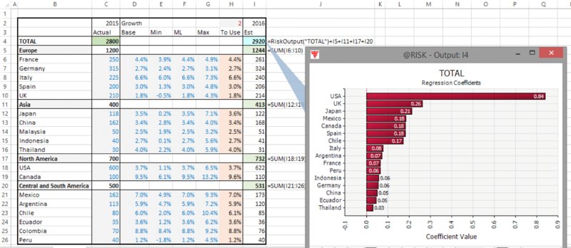
Figure 13.28 Tornado Chart for a Model with Many Line Items
In practice, it might be desired to see such a tornado graph by regional breakdown; however, the regional totals are not model inputs.
The file Ch13.MakeInput.RevenueForecast2.xlsx contains the use of the RiskMakeInput function, which has been placed around the calculations of the regional totals. Figure 13.29 shows the model and the resulting tornado graph (note also the use of the RiskName function used within the RiskMakeInput).
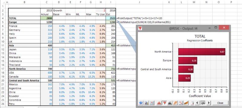
Figure 13.29 Tornado Chart for a Model with Summary Items Using RiskMakeInput
Note that, in practice, the placement of such functions around other formulae (i.e. the parameter of the RiskMakeInput function) may be cumbersome to do and prone to error; an alternative procedure is to create “dummy” cells, which have no role in the actual calculations of the model, but which are cells (placed anywhere in the model) containing RiskMakeInput functions whose parameters are simply references to the original model calculations that are desired to be treated as inputs. This approach produces the same result simply because all precedents to the actual calculation are ignored, with the cells that are turned into inputs providing the post-simulation data that are used to produce the chart.
The file Ch13.MakeInput.RevenueForecast3.xlsx contains an example, shown in Figure 13.30 (the populated cells in column L are the dummy cells); the tornado graph has the same resulting profile as in the earlier example, but no intervention in the model itself is required.
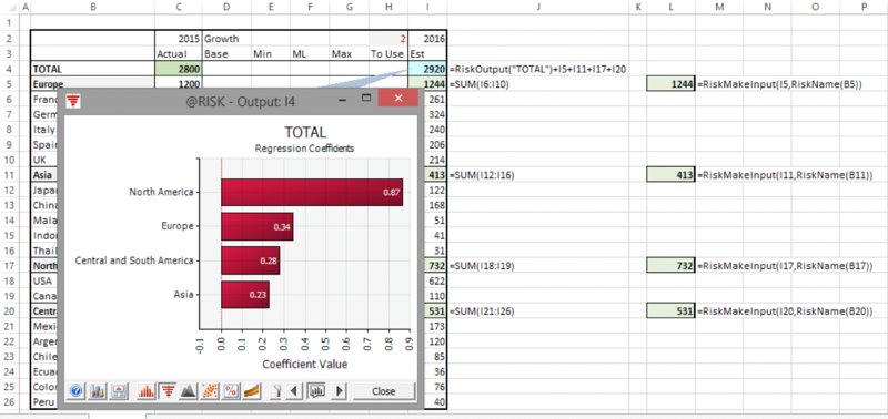
Figure 13.30 Use of RiskMakeInput as Dummy Cells in a Model
Note that scatter plots can also be produced, such as that shown in Figure 13.31 for the total sales against those in the North American region.
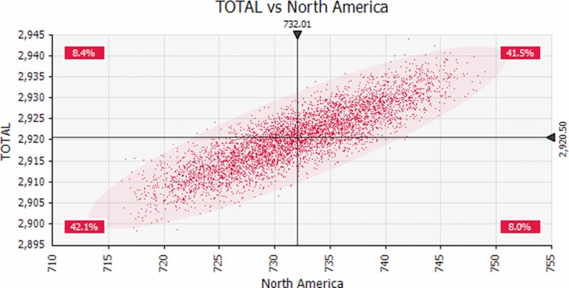
Figure 13.31 Scatter Plot of Total Revenues Against those of North America
The same principles apply in the context of a risk register, as shown below.
The file Ch13.MakeInput.RiskRegister1.xlsx shows a risk register with the tornado graph of the simulated total; by default, every source of risk (i.e. a distribution) is an input, so that the occurrence and the impact are shown with separate bars on the tornado (bar) chart; see Figure 13.32.
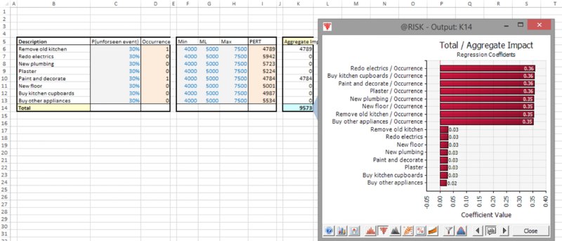
Figure 13.32 Tornado Chart of Risks with Separate Occurrence and Impact Distributions
The file Ch13.MakeInput.RiskRegister2.xlsx contains essentially the same model, but additional cells (column M) are included, which are simple cell references to the calculated column K, and these cells are the arguments to the RiskMakeInput function. Figure 13.33 shows the resulting model and tornado graph.
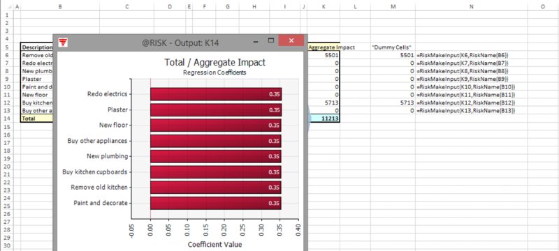
Figure 13.33 Tornado Chart with Occurrence and Impact Aggregated into a Single Risk Factor
Another useful function is RiskCompound. Its basic property is to directly provide the result of adding a number of random samples together. For example, one can test the effect of the addition of two uniform continuous distributions (which we know from Chapter 9 results in a triangular distribution), by simply placing the single formula
in a cell of Excel (in this case, cell C4), and running a simulation. Figure 13.34 shows the result of doing this.
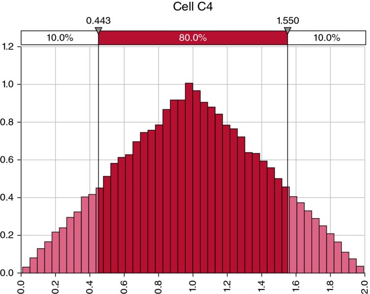
Figure 13.34 A Triangular Process as a Compound Distribution
Of course, the main use of the function concerns cases where both the number of distributions to be added is not fixed and the impact of each is uncertain (and independent of each other):
- If the number of items were known, then one could simply place each underlying impact distribution in a separate cell of Excel and add them up.
- If the impact were a fixed number, then this fixed number could be multiplied by the (uncertain) number of items.
The function adds up independent samples of the impact distributions; one cannot simply multiply the number of items with a single impact number, as this would imply that the impacts of all processes were fully dependent on each other (i.e. all high or all low together), and so would create a wider (typically not appropriate) range.
Applications include operations and insurance:
- The number of customer service calls arriving per minute may be uncertain, as is the time (or resource) required to service them.
- The number of car accidents in a region per month may be uncertain, as is the impact (or insurance loss) for each one.
- Generalised risk registers, in which risks may occur more than once, but each has a separate impact.
The function can also be applied in general business forecasting, where generic items are used. For example, a generic (i.e. unknown and unspecific) new customer may purchase an uncertain amount next year, and one may wish to create a forecast in which the number of new customers is an uncertain figure from within a range of general prospects.
The file Ch13.Compound.RiskRegister.xlsx contains an example in which there is a register of items, where each “risk” may occur more than once (such items could be the number of customers with a certain type of query who call into a customer service centre, for example). The intensity of occurrence is the parameter that is used in the Poisson distributions in column D (this column would contain the Bernoulli distribution in a traditional risk register). Column K contains the RiskCompound function, which adds up a number of independent samples of the impact distributions, with this number being that which is sampled by the Poisson process. Figure 13.35 shows a screen clip of the model and the simulation results. Although it is not shown here, the reader will be able to verify that the tornado diagram of the output treats the items in column K (i.e. the compound distributions) as inputs, so that there is no need to explicitly also use the RiskMakeInput function in order to do so.
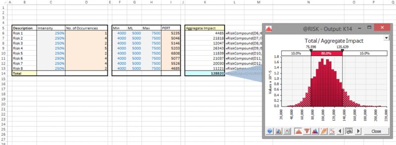
Figure 13.35 A Portfolio of Compound Processes and the Simulated Total Output
13.4.6 Additional Graphical Outputs and Analysis Tools
There is a large variety of other graphical display and reporting possibilities with @RISK. Some of these are:
- Quick Report. This is a useful one-page summary containing key graphs and statistics for any output, including recording the data required to repeat the simulation in principle (i.e. if the model or the modelling environment has not changed).
- Summary Trend plots for time series of data (“fan” charts); an example was used in Chapter 11 in the model concerning the development of market share over time.
- Excel Reports. This toolbar icon allows one to generate a number of reports in Excel.
Additional analysis features (under the Advanced Analyses icon) include:
- Goal Seek. This is analogous to Excel's GoalSeek, and could be used, for example, to find the value required of an input variable so that some target is met in (say) 90% of cases.
- Stress Analysis. This allows one to run simulations to see the effect on an output if the input distributions are restricted to part of the range (such as all being at their P90 point or more).
- Advanced Sensitivity Analysis. This runs several simulations, one for each of a set of values that are input, where such an input can be selected values from a distribution (such as specified percentiles) or static input values.
Each of these procedures generally needs to run several simulations in order to perform the analysis.
The interested reader can explore these further using the manual, in-built examples and Help features within the software.
13.4.7 Model Auditing and Sense Checking
Of course, risk models can become quite complex due to the larger input data areas compared to static models, the potential for more detail to be required on some line items and the need for formulae that work flexibly across a wider variety of input scenarios.
As discussed in Chapter 7, when faced with a model that produces non-intuitive results, the model may be wrong, or one's intuition may be so; in the latter case, the model will often prove to be a valuable tool to develop one's intuition and understanding further.
@RISK has a number of techniques to help gain an overview of a model, consider its integrity and search for errors. Some of the core features include:
- The Model Window icon on the toolbar provides an overview of the distributions in the model. It is instructive to look at the general type of distributions used (discrete, continuous), as this often gives some reasonable indication of the general model context (e.g. risk registers versus continuous uncertainties). One can also see whether there are any correlated items, and which cells are defined as outputs. The knowledge of the desired output (for a model that one has not built oneself) is a very important piece of information; a traditional Excel model does not directly inform one of what the output cell is, whereas this knowledge is fundamental in order to know the objectives of the model.
- Using tornado graphs and scatter plots to gain a quick overview of key risk factors within a model.
- Simulation Data. The toolbar icon allows one access to the simulation data (
 ). One can use this to sort or filter the data (e.g. to find those iterations that generated error values, or other unusual outcomes, and to see the corresponding input values that applied). One can also step through these data, whilst the values in the Excel worksheet update at each step. As an example, in a model with a parameter dependency, if the most likely value of a PERT distribution is varying throughout a simulation (as it is determined from samples of other distributions), but its minimum and maximum values are hard coded and not linked to the most likely value, then cases may arise where the most likely is less than the minimum, so that the distribution cannot be formed and an error arises. These types of errors are made transparent by reviewing the individual iterations that caused errors to arise.
 - On the Simulation Settings/View tab, one can check the boxes corresponding to Show Excel Recalculations or Pause on Output Errors. The first option will slow down the simulation, so should generally not be used as a default setting.
13.5 Working with Macros and the @RISK Macro Language
This section describes some key elements of working with VBA macros when using @RISK, including an introduction to @RISK's own macro language.
13.5.1 Using Macros with @RISK
In principle, the use of macros with @RISK is straightforward. Of course, for many people, one of the reasons to use @RISK is to avoid having to use macros! Nevertheless, on occasion the use of fairly simple macros is helpful or necessary.
In Chapter 7, we mentioned typical cases where macros may be required, such as:
- Before or after a simulation, to toggle the value of a switch, so that risk values are used during the simulation, but that the base case is shown as soon as the simulation has finished running. Similarly, one may need to remove Excel Data/Filters before a simulation, or to run GoalSeek or Solver before or after a simulation, and so on.
- At each iteration of a simulation, to run procedures such as the resolution of circular references, or use GoalSeek or Solver.
In principle, the macros associated with such procedures can be placed at the appropriate place within the SimulationSettings/Macros tab. Figure 13.36 shows an example, in which the procedures used in Chapter 7 to toggle the switch are placed in the tab; when a user runs the simulation (using the Start Simulation icon), the model switch will first be toggled to ensure that the risk values are used, and after the simulation the procedure to toggle to base values will be run.
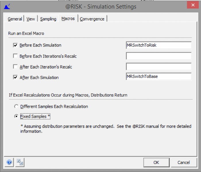
Figure 13.36 The Macros Tab of the SimulationSettings Dialog
Where macros need to be run at each iteration, there is more potential complexity; as discussed in Chapter 7, in general one would wish for the distribution samples to be frozen when such procedures are running. Fortunately, this is easy to achieve in @RISK (versions 6.3 onwards), as one can simply select the Fixed Samples option in the dialog box. (As the dialog box indicates, this would not be a valid procedure if the macro changed the value of distribution parameters, which would be a very unusual situation; even where there are parameter dependencies in the model, since distribution samples are fixed, the parameters of dependent distributions would not change during such recalculations unless the parameters of the independent distributions were changed by the macro.)
In versions prior to 6.3, although a dialog box existed that was superficially similar to the one above, the Fixed Samples option did not exist. In those cases, one generally needed to fix distribution samples using a separate macro to assign values from distributions to fixed cells (analogous to that discussed in Chapter 12), and also would frequently have then created cells that referred directly to these fixed values, which would have been defined as inputs using the RiskMakeInput function, in order to record the sampled values actually used and for purposes of producing graphical output. Fortunately, such procedures are no longer necessary. (An exception to this requirement was when models used Excel iterations to resolve circularities, in which case the fixing procedure was built into @RISK, but not explicit to the user. Note that this process can, however, not be readily observed: whilst Excel's iterative method will resolve in Static view, in the Random view, as Excel iterates to try to resolve the circularity, new samples from the distributions are drawn from each iteration, and hence the target for the iterative process is constantly moving.)
Note also that if one tests models that contain macros by using F8 in VBA to step through it, one may observe results that are not the same as those that would occur when the simulation is actually run: stepping through may cause the worksheet to update, which would often lead to the distributions being resampled, whereas during the simulation, the values would be fixed when using the Fixed Samples option.
13.5.2 The @RISK Macro Language or Developer Kit: An Introduction
In the above, we discussed the use of @RISK functionality to manage the sequencing of general VBA macros. In addition, @RISK has its own macro language, known as the VBA Macro Language or the @RISK for Excel Developer Kit (XDK). Information about this can be found under the general Help menu within @RISK, as shown in Figure 13.37.
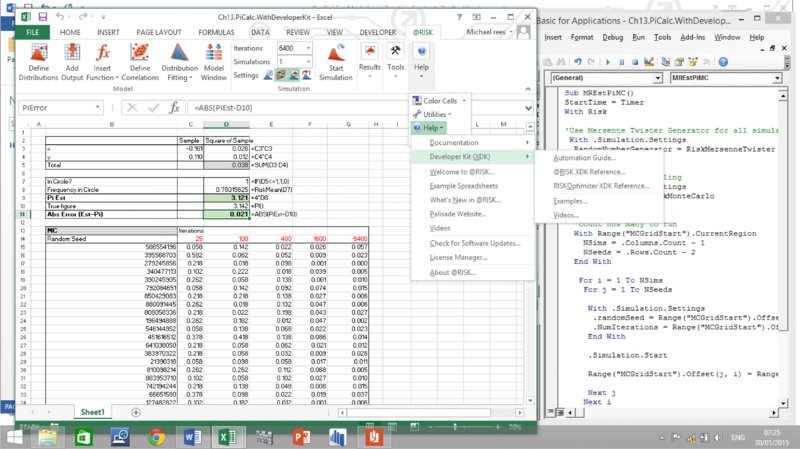
Figure 13.37 Accessing the XDK Help Menu
Some general uses of these tools could be:
- To create a “black-box” interface in which the user needs only to press a button in Excel to launch a macro to run the simulation. Such a macro could also ask the user for information (such as the desired number of iterations, or the sampling type desired to be used, etc.), so that the user does not have to directly interface with (or learn) the @RISK toolbar.
- To change Simulation Settings at run time, so that the same defaults are used, irrespective of what is currently set on the toolbar.
- To generate output statistics and reports.
- To automate other procedures that would be time-consuming to implement.
In the following, we provide examples of the use of these tools to repeatedly run simulations, to change aspects of the random number sampling and generator methods and to generate reports of the simulation data.
13.5.3 Using the XDK to Analyse Random Number Generator and Sampling Methods
In this section, we use the XDK to show how one may compare the effectiveness of the random number generation methods in @RISK.
We start by noting that a particular case of a simulation model in which the true value of the output is known is that in which one estimates the value of π (3.14159…) by the “dartboard” method:
- Draw random samples of x and y from uniform continuous distributions between minus one and plus one (these represent the final position that the dart lands within a square).
- For each draw, test whether the sum of the squares of the two variables is less than one: when centred at the origin, the circle is defined by x and y points, which satisfy x2 + y2 = 1, so this can be used to test whether the dart lands within the circular dartboard.
- Use the RiskMean function to report the frequency with which the test shows that the sum is within the circle, and multiply this by four. At the end of the simulation the frequency with which this is the case will be approximately π/4 (because a circle of radius one has an area equal to π, whereas the square drawn around that circle has area four).
The file Ch13.PiCalc.xlsx contains these calculations, with an example post-simulation shown in Figure 13.38.
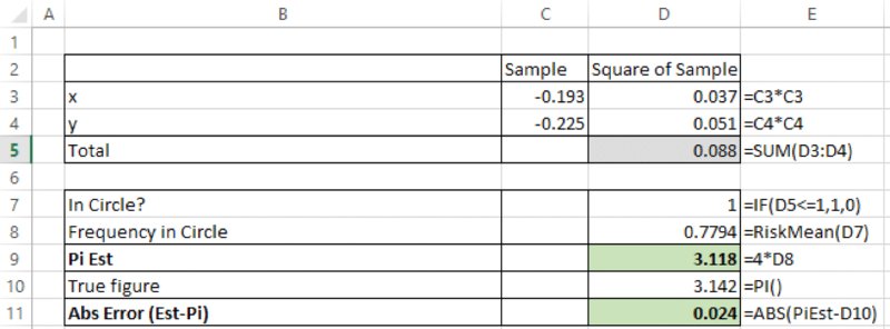
Figure 13.38 Model to Calculate π Using the Dartboard Method
In order to test the effectiveness of each sampling type (MC or LH, discussed earlier in the chapter), one could perform the same calculations several times with each, and measure the run time and accuracy:
- Run a simulation using each type, where each simulation uses the same seed value.
- Measure the run time of each simulation.
- Calculate the error compared with the true value.
- Repeat the above in an automatic fashion many times over, using a new random number seed each time, and compare the accuracy of the results against the time taken.
The file Ch13.PiCalc.2DResultsTable.xlsx contains the results of running 30 simulations for each method, and for various numbers of iterations. The summary results are shown in Figure 13.39. (The same set of randomly chosen seeds was used for each sampling method, shown in the results tables in column B.) The summary table shows the average (over 30 simulations) of the error (in absolute terms) for the MC and the LH sampling types, for various numbers of iterations, as well as the total run time. (Such a comparison is, of course, still imperfect, as run time may be affected by other processes that were occurring on the computer at the same time.)
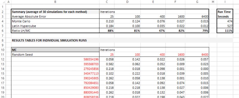
Figure 13.39 Summary Results of the Two-dimensional Dartboard Method
As mentioned in Chapter 6, as the number of iterations increases by multiples of four (i.e. from 25 to 100 to 400, and so on), the error should generally be half (the inverse square root law). This is broadly confirmed in this case: if one considers the error values of the LH method, comparing column G (6400 iterations) with column C (25 iterations), the error ratio is 0.012/0.184 (around 6.6%); this corresponds to halving the original error (0.184) four times over, i.e. to one-sixteenth of the original value.
From this particular experiment, one would conclude that LH generally reduces the statistical error by about 20% compared to MC at the expense of approximately 10% more computational time (the computational time in this case is dominated by the cases in which 6400 iterations were run). Note that one may state this in an alternative way: to reduce the error to 80% of the original value would generally require (using the inverse square root law) that the number of iterations be increased by approximately 56% (as ![]() . Thus, one would conclude that it would be more efficient (from a time perspective) to use an LH method (requiring 10% extra time) than additional iterations of the MC method (requiring 56% extra time).
. Thus, one would conclude that it would be more efficient (from a time perspective) to use an LH method (requiring 10% extra time) than additional iterations of the MC method (requiring 56% extra time).
The above experiment involves repeated running of simulations in which each one required changing (compared to the immediately prior one) at least one of the seed values, or the number of iterations, or the sampling type. Of course, this could be done manually, but clearly it would be very cumbersome (and one would also have to measure the run time precisely). The XDK is therefore ideal for such an experiment.
The file Ch13.PiCalc.2D.WithDeveloperKit.xlsm contains the implementation of the above procedure using the XDK. (When using the XDK, one needs to create a reference to the @RISK add-in [under Tools/References within the Visual Basic Editor], in order to access the @RISK object model; this step is not shown here.) Figure 13.40 shows a screen clip of the file, from which one can see that buttons have been created so that the user can run subroutines for both the MC and LH sampling types, or run them individually.
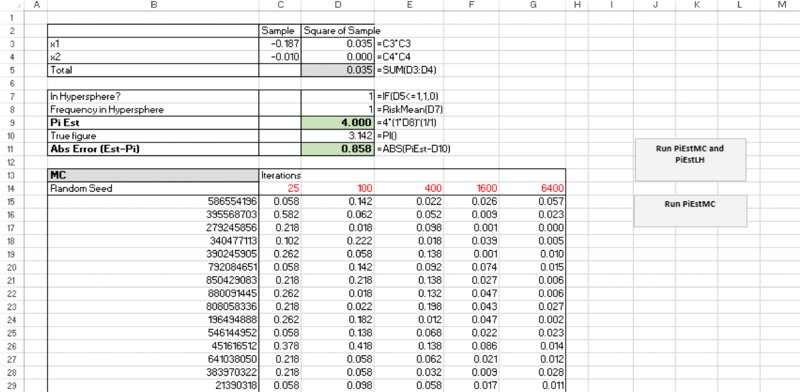
Figure 13.40 Model Used to Run the Two-dimensional Dartboard Method
The code used in the file is split across two (essentially identical) subroutines, one that runs the simulations in the case that Monte Carlo sampling was used and the other for Latin Hypercube.
Thus, the master routine to run both is:
Sub MRRunBoth()
 Call MREstPiMC
 Call MREstPiLH
End Sub
with the full code for the MC-related simulations being:
Sub MREstPiMC()
StartTime = Timer
With Risk
'Use Mersenne Twister Generator for all simulations
 With .Simulation.Settings
 .RandomNumberGenerator = RiskMersenneTwister
 End With
'Run Monte Carlo Sampling
 With .Simulation.Settings
  .SamplingType = RiskMonteCarlo
  End With
  'count how many to run
  With Range("MCGridStart").CurrentRegion
    NSims = .Columns.Count - 1
    NSeeds = .Rows.Count - 2
  End With
   For i = 1 To NSims
    For j = 1 To NSeeds
     With .Simulation.Settings
      .randomSeed = Range("MCGridStart").Offset(j, 0)
      .NumIterations = Range("MCGridStart").Offset(0, i)
     End With
     .Simulation.Start
     Range("MCGridStart").Offset(j, i) = Range("PiError")
     Next j
    Next i
End With 'end Risk
EndTime = Timer
Range("RunTimeMC") = EndTime - StartTime
End Sub
Analogous code applies for the LH-related simulations, with a simple adaptation of the line referring to the sampling type, from RiskMonteCarlo to RiskLatinHypecube, as well as adapting the ranges referred to for the data requirements and storage, i.e. the predefined Excel-named ranges MCGridStart (cell B13) and LHGridStart (cell B48).
From this example, some key syntax within the XDK should be visible, such as how to set the random number generator method, the sampling type, the number of iterations and how to run (start) a simulation. The VBA Timer function is used to measure the total elapsed time for the run of all simulations and all iterations for each method.
With respect to the comparison of MC with LH methods, one may argue that the above test unfairly favours LH sampling, as it is only conducted with respect to two uncertain variables (or dimensions): as stated earlier, the stratification process used by @RISK's LH sampling type is done as a one-dimensional process for each variable, so that its effect would be diminished in multi-variable models. In fact, it is possible to generalise the experiment to have more variables, so that the comparison would be fairer in more general cases where there are multiple sources of uncertainty. For example, instead of referring to a circular “dartboard” (in two dimensions), one could refer to a sphere (in three dimensions), whose volume is ![]() , where VU3 refers to the volume of the unit sphere in three dimensions; the box surrounding this sphere would have volume 8 (i.e. 23), so that the “dart” should land within the sphere with a frequency of
, where VU3 refers to the volume of the unit sphere in three dimensions; the box surrounding this sphere would have volume 8 (i.e. 23), so that the “dart” should land within the sphere with a frequency of ![]() , or
, or ![]() .
.
In fact, one can generalise this further. In four dimensions the volume of the unit sphere is given by ![]() , whereas that of the surrounding box is 16, and in five dimensions,
, whereas that of the surrounding box is 16, and in five dimensions, ![]() (thus, the power term relating to π increases by one for every two increases in dimension). Thus, to test the effect of MC versus LH in multi-variable models, we shall work in even dimensions only, using the formula:
(thus, the power term relating to π increases by one for every two increases in dimension). Thus, to test the effect of MC versus LH in multi-variable models, we shall work in even dimensions only, using the formula:
where N is the (even) number of variables (dimensions), n = N/2 (or N = 2n) and ! denotes the factorial.
The volume of the surrounding box is 2N. Thus, the frequency, f, with which the dart lands within the hypersphere is given by:
Thus, where fest is the estimated frequency (i.e. as measured in the simulation), the estimated value of π (πest) would be given by πest= 4![]() .
.
In principle, therefore, a multi-dimensional test is straightforward to conduct. In fact, the practical challenge is that the value of f rapidly becomes small as N (2n) becomes large, as shown in Figure 13.41. Thus, the number of iterations needed would become large.
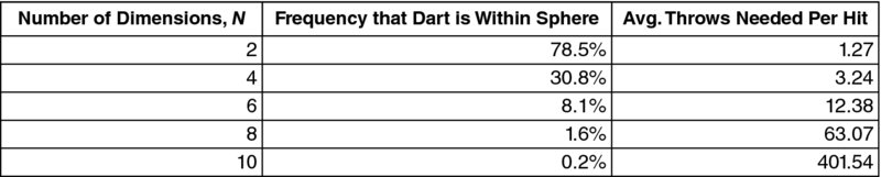
Figure 13.41 Expected Frequency of Hits with the Multi-dimensional Dartboard Method
The file Ch13.PiCalc.10D.WithDeveloperKit.2.xlsm contains the model necessary to test the above with 10 input variables (i.e. where the “dartboard” is a 10-dimensional hypersphere). Due to the low frequency of hitting the target (i.e. approximately 0.2%), the model has been run with 102,400 iterations (i.e. 6400 times 16), and for the same 30 seeds as in the above example. In addition, the summary statistic (absolute error and run time) is recorded for each simulation. Figure 13.42 shows a screen clip of the model, which is laid out slightly differently to the earlier example. To minimise the effect of any cases where the computer processor is tied up with some other activity, the simulation runs alternately between the MC and LH sampling type (rather than doing all the MC simulations followed by all the LH ones, as done above). Row 35 contains the header fields that are used to predefine most of the named ranges that are used within the code (which is shown below).
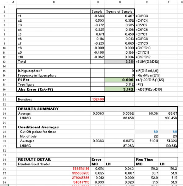
Figure 13.42 Summary Results of the 10-dimensional Dartboard Method
Sub MRRunBoth()
With Risk
 'Use Mersenne Twister Generator for all simulations, and fix number of iterations
  With .Simulation.Settings
  .RandomNumberGenerator = RiskMersenneTwister
  .NumIterations = Range("NIterations").Value
  End With
 'Initiate runtime tracking variable
  RunTime = 0
 'count how many simulations to run, according to seed list
  With Range("SeedListHeader").CurrentRegion
   NSeeds = .Rows.Count - 2
  End With
 For i = 1 To NSeeds ' Run simulation for each sampling type
  With .Simulation.Settings
    .randomSeed = Range("SeedListHeader").Offset(i, 0)
  End With
 '############# DO MC SAMPLING METHOD
 'Set sampling to Monte Carlo
  With .Simulation.Settings
   .SamplingType = RiskMonteCarlo
  End With
 ' Measure time and run simulation, and record error
  StartTime = Timer
  .Simulation.Start
  EndTime = Timer
  RunTime = EndTime - StartTime
  Range("ErrorHeaderMC").Offset(i, 0) = Range("PiError")
  Range("RunTimeHeaderMC").Offset(i, 0) = RunTime

 '############# DO LH SAMPLING METHOD
  With .Simulation.Settings
   .SamplingType = RiskLatinHypercube
  End With
 ' Measure time and run simulation, and record error
  StartTime = Timer
  .Simulation.Start
  EndTime = Timer
  RunTime = EndTime - StartTime
  Range("ErrorHeaderLH").Offset(i, 0) = Range("PiError")
  Range("RunTimeHeaderLH").Offset(i, 0) = RunTime
 Next i 'next seed value
End With 'Risk
End Sub
In terms of aggregate results, we can note (row 24 and row 25) that there is essentially no difference in accuracy, or average run time requirements, between the approaches. A closer inspection of the data sets reveals that most run times are around 50 seconds, but some are significantly higher; row 30 and row 31 contain the averages that apply when run times above 60 seconds are excluded (perhaps other processes were running in the background during such runs); however, doing so does not change the general picture.
The results would seem to suggest that there is little to choose between the sampling types, with one being as good as the other. Note that the structure of this test arguably favours MC methods slightly, as the model used is small (in terms of the number of calculations that are performed once the random samples are generated); in a larger model, the proportion of time spent generating random numbers (compared to the total run time including recalculating the model) would be less than in a small model, and so the total MC computational time would be closer to that of LH, even as the LH accuracy may be marginally better.
As a conclusion, it would seem that LH is a marginally superior method when there are small numbers of model variables (fewer than about 10), whereas for larger numbers of variables, there is little difference between the methods. Interested readers (with sufficient time) can, of course, test these issues for themselves, as the basic infrastructure to do so is provided within the model (for example, more iterations and simulations with different seed values could be run, or the number of dimensions increased).
13.5.4 Using the XDK to Generate Reports of Simulation Data
Another powerful use of the XDK is to generate reports or other aspects of simulation data, as shown in the following example.
The file Ch13.XDK.PreGenerateCorrelRands.xlsm contains code that would allow one to generate a set of correlated random numbers and store their values in a data worksheet. One application of this may be if one needs to work with “frozen” random numbers (as covered earlier in the chapter and in the text), if other procedures need to be run at each iteration. In such cases, one could pregenerate all the numbers and then use them in sequence as fixed numbers in a subsequent simulation. Figure 13.43 shows an example. Row 4 contains five random variables (PERT distributions) that are correlated in accordance with the correlation matrix shown. The button runs the macro GenerateData that instructs the XDK to run a simulation (which generates the correlated samples) and then to generate a report of the data in Excel (in order to set the required sample size, the user inputs the value in the cell named NSamples, containing the value 20 in the screen clip); the code is shown below.
Figure 13.43 Model to Generate a Set of Correlated Random Numbers
Sub GenerateData()
With Risk
'Ensure that sheet containing the data gets written into the same workbook
 With .ApplicationSettings
  .ReportPlacement = RiskActiveWorkbook
  .ReportOverwriteExisting = True
 End With
 With .Simulation.Settings
  .NumIterations = Range("NSamples").Value
 End With
 .Simulation.Start
 .GenerateExcelReports RiskSimulationReportData
End With
End Sub
The XDK has many other options that the interested reader can further explore by referring to the Help menu and the manual associated with it.
13.6 Additional In-Built Applications and Features: An Introduction
This section provides an overview of some other application areas and features that are built into the @RISK software.
13.6.1 Optimisation
As mentioned in various places in this text, there is a close link between optimisation and risk modelling:
- Optimisation modelling arises in the case where some of a model's inputs are choice variables (such as the launch dates that one may choose to launch a project, or the percentage participation that one may wish to take in an asset or business project).
- Risk modelling arises when a model has inputs whose values are uncertain (and may be controllable only by adjusting the context in which one operates), as discussed throughout this book.
Many real-life situations may contain both optimisation and uncertainty characteristics. In many cases, it can be challenging to create a single model that is valid for all possible cases; for example, so that the uncertainty profile is correctly captured for whatever selection of choice variables (decisions) is made. For this reason, heuristic (pragmatic) techniques are often used, and they can be reasonably accurate (partly due to the flat nature of any optimisation curve around its optimal point, as mentioned in Chapter 6).
Nevertheless, on occasion, one can build models whose inputs consist of both choice and uncertain variables, and where the uncertainty profile is accurately captured for all combinations of choice variables. This is particularly applicable when a model consists of summing a set of independent items or projects, as is the case in many portfolio situations (where the total portfolio output is simply the sum of the elements). Thus, if each project in the portfolio is independent, aspects of the portfolio construction can be considered to be an optimisation problem.
An example was provided in Chapter 4, where we presented a set of independent projects and considered the optimisation of their launch dates (using Solver). Such a solution could also have been searched for using Palisade's Evolver tool, which is part of the DecisionTools Suite, of which @RISK is also a part.
On the other hand, when aspects of each project are uncertain (such as the initial investment required or the future cash flow profile), then the optimisation has to take this into account. In standard financial portfolio theory, many of the associated optimisation algorithms make use of the underlying mathematics embedded in a situation. However, in the most general case, one may have to repeatedly create a set of trial values to act as a test of the optimal solution, run a simulation to see the uncertainty profile that would result for this set of trial assumptions and repeat this for other sets of trial values. Of course, the choice of which solution is optimal will depend on the user defining appropriate criteria, which relate to statistics of the distribution of output; for example, one may wish to find the solution that maximises the average or minimises the variability (standard deviation) of some project metric (such as cash flow in a particular year, or net present value).
The process of generating sets of trial values in an automated way, and of running a simulation for each set of trial values, is facilitated by the use of the RiskOptimizer tool that is embedded within @RISK Industrial. The trial values generated are not totally random, but partly use information about previous trial solutions to generate others, and therefore are more efficient than simply running many simulations to do so (i.e. in theory, one could generate trial values by one random sampling process, fix them and then run a full simulation, before moving to a new set of randomly generated trial values).
The tool is fairly straightforward to use, once the model has been created in a valid way (for example, so that project launch dates can be changed, if these items are to be optimised, as discussed in the example in Chapter 4), the optimisation criteria are set and constraints defined. In this context, as mentioned earlier in the text, it can be important to try to understand (at an intuitive level) what effect any uncertainty would have on the final optimal solution, as there is a potential to create unnecessary complexity otherwise. For example, the optimal route to travel across a town may be the same independently of whether one considers the travel time on each segment to be fixed or whether one considers it to be uncertain. On the other hand, this conclusion can be changed by risk tolerances and/or non-symmetry of the uncertainties, as well as non-linearities in the modelling situation: for example, for the sake of always arriving on time, one may decide to cycle to work, even though, on average, it takes longer than taking the train, because in some cases the train journey is subject to severe disruption. In these cases, optimisation tools are powerful methods, as pragmatic techniques may be insufficient.
13.6.2 Fitting Distributions and Time Series to Data
@RISK has two main categories of fitting capabilities:
- Distribution fitting.
- Time series fitting.
Each of these is fairly straightforward from the perspective of the software mechanics, although the underlying theory and concepts concerning the various fitting procedures and criteria are more complex, and are beyond the scope of this text. Note that fitting procedures take into account the full set of data, unlike some of the approaches to parameter matching that were discussed in Chapter 9.
In the following, we simply make several remarks that relate most directly to modelling issues.
When using distribution fitting, one (implicitly) assumes that data points are independent of each other, and are all random samples drawn from the same distribution with the same parameters. The procedure then finds, for each distribution tried, the parameters of that distribution that would best fit the data, before ranking the fits (of the best fitting) of these distributions. As mentioned in Chapter 9, when using fitting as a distribution selection tool, in practice one may sometimes simply use the best fitting distribution, whereas for others, one may believe that it is appropriate to combine the fitting process with other aspects of distribution selection (such as the use of scientific or conceptual methods). One is also implicitly assuming that the underlying distribution that generates the data set is one of those available in the fitting procedure (so, for example, one would not directly find a reasonable fit to compound processes). Finally, as noted in Chapter 9, any procedure based on data implicitly assumes the integrity and validity of the data.
The Time Series fitting procedures apply to a set of data points that have occurred in time (and that are not independent of each other, in the sense that the order in which they occurred is necessary to take into account the fit, unlike for simple distribution fitting). One can then find the best fitting times series, for a single series, or use the Batch Fit when data from several series are available; if a correlation is found between them, the fitting tool can also generate correlated time series.
Note that, in general, the creation of many time series processes does not explicitly require @RISK's time series functionality, as the examples discussed in Chapter 11 show. However, the ability to find (through fitting) the appropriate time series to create is an important feature of the software.
In the case that one wishes to create a time series directly, this can be done in a similar way to Chapter 11, as discussed below.
The file Ch13.TimeSeries.MA1.xlsx contains an example of the first-order moving average function that was also implemented using Excel in Chapter 11. These functions are array functions; at the time of writing they are not allowed to be set directly as simulation outputs; one can instead create a cell reference to them, and set this cell as an output; see Figure 13.44.
Figure 13.44 Example of Moving Average Time Series Using @RISK
13.6.3 MS Project Integration
As discussed earlier in the text, project schedules (and integrated cost analysis) can be built in Excel, provided that the project structure is sufficiently simple; indeed, a simulation of the schedule can be done in such a case (see the example in Chapter 4).
However, very often, project structures are such that a change in an input assumption (such as the length of a task duration) would alter the critical path in the project, perhaps by changing the branching structure. For example, a failure at the product testing stage may mean that one needs to branch to a product redesign task. In such cases, tools such as Microsoft Project can be very useful, as they are specifically designed to capture such linkages.
@RISK's Project capability allows a user who has both MS Project and @RISK to work with files that are essentially linked; the .mpp file can be “imported” so that it appears in Excel and the task durations can be changed (in Excel), with the project schedule recalculating in MS Project and then updating in Excel as well; both applications are open simultaneously.
Note that this tool could be used to create an integrated cost-schedule model in Excel, so that task durations (or costs) could be changed, or sensitivity analysis of the items run, even where none of @RISK's risk or simulation capability was used. A simulation can, of course, also be run; typically the end date of a project or a subtask (as well as some cost estimates) would be set as outputs and simulated, distributions of each calculated and scatter plots (e.g. of cost and schedule) shown, as demonstrated in Chapter 4.
13.6.4 Other Features
As stated earlier, this text has not tried to cover all aspects of @RISK comprehensively. Readers wishing to know more can refer to the Help menu within the software, and the various files, other utilities and resources that are provided with it, as well as the Palisade website and its associated resources.
13.7 Benefits of @RISK over Excel/VBA Approaches: A Brief Summary
The following is a brief summary of some key points relating to the benefits of using @RISK versus (the cost-free and ubiquitous) Excel/VBA. The list is not intended to be totally exhaustive, but to highlight many of the key points made at various places in the text:
- The use of @RISK facilitates many aspects of the processes of building risk models and communicating their content, concepts and results. It generally makes key steps easier, quicker, more transparent and more robust, especially due to the graphics capabilities and statistical tools, as well as the ease of creating relationships of sampling dependencies.
- There is a large set of distributions and parameters available, and the percentile (alternate) parameter form is available for most distributions. Some special distributions would also be cumbersome to replicate with Excel/VBA approaches.
- Many aspects of the simulation and random number selection are easy to control, including the ability to repeat a simulation exactly, to conduct multiple simulations, to select the random number generation algorithms and the sampling type. In addition, it is straightforward to embed within the simulation procedures that need to be run at each iteration.
- There are tools to assist in the auditing of models, and to conduct enhanced results analysis.
- Additional functionality includes the ability to fit distributions and time series to data, to conduct optimisation under uncertainty and to integrate Microsoft Project with Excel. Clearly, much of this functionality would (at best) be extremely complex and time-consuming to implement in Excel/VBA, and attempting to do so would likely detract from the core task of providing value-added decision support.
- Models can generally be structured without particular consideration given to where risk distributions are placed within them, or to whether their ranges need to be contiguous to each other.
- There is generally no VBA coding required (although basic VBA can be useful on occasion, even where not strictly necessary).
- It is a tried and tested application, whereas bespoke-written VBA code is more likely to contain coding errors or not be robust.
In summary, more time can be focused on generation of insights, solutions and recommendations, and creating value-added in a business and organisational context.