
Chapter 2. Enterprise Layer 2 and Layer 3 Design
In network design, it is common that a certain design goal can be achieved “technically” using different approaches. Although, from a technical deployment point of view this can be seen as an advantage, from networks’ design perspective on the other hand, almost always one of the most challenging parts is, which design option should be selected? (To achieve a business driven design that takes into considerations technical and non-technical design requirements.) Practically, to achieve this, network designers must be aware of the different design options and protocols as well as the advantages and limitations of each. Therefore, this chapter will concentrate specifically on highlighting, analyzing, and comparing the various design options, principles, and considerations with regard to Layer 2 and Layer 3 control plane protocols from different design aspects, focusing on enterprise grade networks.
Enterprise Layer 2 LAN Design Considerations
To achieve a reliable and highly available Layer 2 network design, network designers need to have various technologies in place that protect the Layer 2 domain and facilities having redundant paths to ensure continuous connectivity in the event of a node or link failure. The following are the primary technologies that should be considered when building the design of Layer 2 networks:
![]() Layer 2 control protocols, such as Spanning Tree Protocol
Layer 2 control protocols, such as Spanning Tree Protocol
![]() VLANs and trunking
VLANs and trunking
![]() Link aggregation
Link aggregation
![]() Switch fabric (discussed in Chapter 8, “Data Center Networks Design”)
Switch fabric (discussed in Chapter 8, “Data Center Networks Design”)
Spanning Tree Protocol
As a Layer 2 network control protocol, the Spanning Tree Protocol (STP) is considered the most proven and commonly used control protocol in classical Layer 2 switched network environments, which include multiple redundant Layer 2 links that can generate loops. The basic function of STP is to prevent Layer 2 bridge loops by blocking the redundant L2 interface to a level that can provide a loop-free topology. There are multiple flavors or versions of STP. The following are the most commonly deployed versions:
![]() 802.1D: The traditional STP implementation
802.1D: The traditional STP implementation
![]() 802.1w: Rapid STP (RSTP) supports large-scale implementations with enhanced convergence time
802.1w: Rapid STP (RSTP) supports large-scale implementations with enhanced convergence time
![]() 802.1s: Multiple STP (MST) permits very large-scale STP implementations
802.1s: Multiple STP (MST) permits very large-scale STP implementations
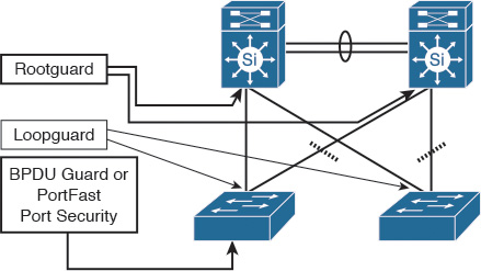
In addition, there are some features and enhancements to STP that can optimize the operation and design of STP behavior in a classical Layer 2 environment. The following are the primary STP features:
![]() Loop Guard: Prevents the alternate or root port from being elected unless bridge protocol data units (BPDUs) are present
Loop Guard: Prevents the alternate or root port from being elected unless bridge protocol data units (BPDUs) are present
![]() Root Guard: Prevents external or downstream switches from becoming the root
Root Guard: Prevents external or downstream switches from becoming the root
![]() BPDU Guard: Disables a PortFast-enabled port if a BPDU is received
BPDU Guard: Disables a PortFast-enabled port if a BPDU is received
![]() BPDU Filter: Prevents sending or receiving BPDUs on PortFast-enabled ports
BPDU Filter: Prevents sending or receiving BPDUs on PortFast-enabled ports
Figure 2-1 briefly highlights the most appropriate place where these features should to be applied in a Layer 2 STP-based environment.
Note
Cisco has developed enhanced versions of the STP. It has incorporated a number of these features into it using different versions of STP that provide faster convergence and increased scalability, such as Per-VLAN Spanning Tree Plus (PVST+) and Rapid PVST+.
VLANs and Trunking
A Layer 2 virtual local-area network (VLAN) is considered as a type of network virtualization technique that provides logical separation with broadcast domains and policy control implementation. In addition, VLANs offer a degree of fault isolation at Layer 2 that can contribute to the optimization of network performance, stability, and manageability. Trunking, however, refers to the protocols that enable the network to extend VLANs across Layer 2 uplinks between different nodes by providing the ability to carry multiple VLANs over a single physical link.
From a design best practices perspective, VLANs should not span multiple access switches; however, this is only a general recommendation. For example, some designs dictate that VLANs must span multiple access switches to meet certain application requirements. Consequently, understanding the different Layer 2 topologies and the impact of spanning VLANs across multiple switches is a key aspect for Layer 2 design. This aspect (applicability and its implications) is covered in more detail later in this chapter (in the section “Enterprise Layer 2 LAN Common Design Options”).
Link Aggregation
The concept of link aggregation refers to the industry standard IEEE 802.3ad, in which multiple physical links can be grouped together to form a single logical link. This concept offers a cost-effective solution by increasing cumulative bandwidth without requiring any hardware upgrades. The IEEE 802.3ad Link Aggregation Control Protocol (LACP) offers several other benefits, including the following:
![]() An industry standard protocol that enables interoperability of multivendor network devices
An industry standard protocol that enables interoperability of multivendor network devices
![]() The optimization of network performance in a cost-effective manner by increasing link capacity without changing any physical connections or requiring hardware upgrades
The optimization of network performance in a cost-effective manner by increasing link capacity without changing any physical connections or requiring hardware upgrades
![]() Eliminate single points of failure and enhance link-level reliability and resiliency
Eliminate single points of failure and enhance link-level reliability and resiliency
Although link aggregation is a simple and reasonable mechanism to increase bandwidth capacity between network nodes, each individual flow will be limited to the speed of the utilized member link by that flow, based on the load-balancing hashing algorithm used unless the flowlet concept is considered1.
1. “Dynamic Load Balancing Without Packet Reordering,” IETF Draft, chen-nvo3-load-banlancing, http://www.ietf.org
Note
In addition to LACP (the industry standard link aggregation control protocol), Cisco has developed a proprietary link aggregation protocol called Port Aggregation Protocol (PAgP). Both protocols have different operational modes, which the network designer must be aware.
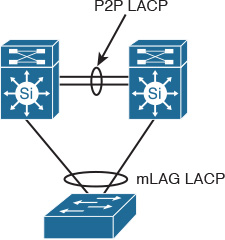
There are two primary types of link aggregation connectivity models:
![]() Single-chassis link aggregation: The typical link aggregation type of connectivity that connects two network nodes in a point-to-point manner.
Single-chassis link aggregation: The typical link aggregation type of connectivity that connects two network nodes in a point-to-point manner.
![]() Multichassis link aggregation: Also referred to as mLAG, this type of link aggregation connectivity is most commonly used when the upstream switches (typically two) are deployed in “switch clustering” mode. This connectivity model offers a higher level of link and path resiliency than the single-chassis link aggregation.
Multichassis link aggregation: Also referred to as mLAG, this type of link aggregation connectivity is most commonly used when the upstream switches (typically two) are deployed in “switch clustering” mode. This connectivity model offers a higher level of link and path resiliency than the single-chassis link aggregation.
Figure 2-2 illustrates these two link aggregation connectivity models.
First Hop Redundancy Protocol and Spanning Tree
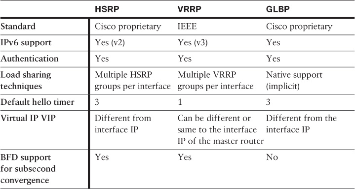
First-hop Layer 3 routing redundancy is designed to offer transparent failover capabilities at the first-hop Layer 3 IP gateways, where two or more Layer 3 devices work together in a group to represent one virtual Layer 3 gateway. Hot Standby Router Protocol (HSRP), Virtual Router Redundancy Protocol (VRRP), and Gateway Load Balancing Protocol (GLBP) are the primary and most commonly used protocols to provide a resilient default gateway service for endpoints and hosts.
Table 2-1 summarizes and compares the main capabilities and functions of these different FHRP protocols.
One of the typical scenarios in classical hierarchal networks is when FHRP works in conjunction with STP to provide a redundant Layer 3 gateway services. However, some Layer 2 design models require special attention in terms of VLANs design (extending Layer 2 VLANs across access switches or not) and the placement of the demarcation point between Layer 2 and Layer 3. (For example, if the interswitch link between the distribution layer switches is configured as Layer 2 or Layer 3 link.) The aforementioned factors can affect the overall reliability and convergence time of the Layer 2 LAN design. The following design model (depicted in Figure 2-3) is considered one of the common design models that has a proven ability to provide the most resilient design when FHRP is applied to an STP-based Layer 2 network (such as VRRP or HSRP). This design model has the following characteristics:
![]() The interswitch link between the distribution switches is configured as Layer 3 link.
The interswitch link between the distribution switches is configured as Layer 3 link.
![]() No VLAN spanning across switches.
No VLAN spanning across switches.
![]() The STP root bridge is aligned with active FHRP instance for each VLAN.
The STP root bridge is aligned with active FHRP instance for each VLAN.
![]() Uplinks from access to distribution are both forwarding from STP point of view.
Uplinks from access to distribution are both forwarding from STP point of view.
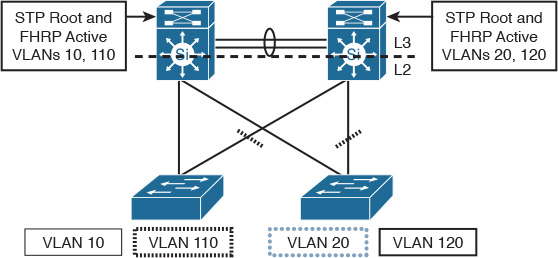
In the design illustrated in Figure 2-3, when GLBP is used as the FHRP, it is going to be less deterministic compared to HSRP or VRRP because the distribution of Address Resolution Protocol (ARP) responses is going to be random.
Enterprise Layer 2 LAN Common Design Options
Network designers have many design options for Layer 2 LANs. This section will help network designers by highlighting the primary and most common Layer 2 LAN design models used in traditional and today’s LANs, along with the strengths and weaknesses of each design model.
Layer 2 Design Models: STP Based (Classical Model)
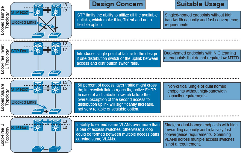
In classical Layer 2 STP-based LAN networks, the connectivity from the access to the distribution layer switches can be designed in various ways and combined with Layer 2 control protocols and features discussed earlier to achieve certain design functional requirements. In general, there is no single best design that someone can suggest that can fit every requirement, because each design is proposed to resolve a certain issue or requirement. However, by understanding the strengths and weaknesses of each topology and design model (illustrated in Figure 2-4), network designers may then always select the most suitable design model that meets the requirements from different aspects, such as network convergence time, reliability, and flexibility. This section highlights the most common classical Layer 2 design models of LAN environments with STP, which can be applied to enterprise Layer 2 LAN designs.
Note
All the Layer 2 design models in Figure 2-4 share common limitations: the reliance on STP to avoid loss of connectivity caused by Layer 2 loops and the dependency on Layer 3 FHRP timers, such as VRRP to converge. These dependences naturally lead to an increased convergence time when a node or link fails. Therefore, as a rule of thumb, tuning and aligning STP and FHRP timers is a recommended practice to overcome these limitations to some extent.
Figure 2-4 summarizes some of the design concerns and lists suggested usage of each of the depicted design models in this figure [5].
Layer 2 Design Model: Switch Clustering Based (Virtual Switch)
The concept of switch clustering significantly changed the Layer 2 design model between the access and distribution layer switches. With this design model, a pair of upstream distribution switches can appear as a one logical (virtual) switch from the access layer switch point of view. Consequently, this approach transformed the way access layer switches connect to the distribution layer switches, because there is no reliance on STP and FHRP anymore, which means the elimination of any convergence delays associated with STP and FHRP. In addition, from the uplinks and link aggregation perspective, one access switch can be connected (multihomed) to the two clustered distribution switches as one logical switch using one link aggregation bundle over multichassis link aggregation (mLAG), as illustrated in Figure 2-5.
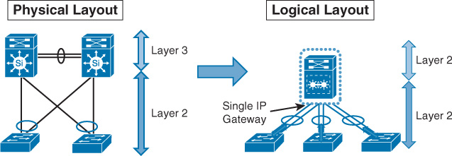
As Figure 2-5 shows, all uplinks will be in forwarding state across both distribution switches from a Layer 2 point of view. There will be one virtual IP gateway that should permit the forwarding across both switches from the forwarding plane perspective. It is obvious that this design model can enhance network resiliency and convergence time, and maximize bandwidth capacity, by utilizing all uplinks. In addition, this design model supports the extension of the Layer 2 VLAN across access switches safely, without any concern about forming any Layer 2 loop. This makes the design model simple, reliable, easy to manage, and more scalable as compared to the classical STP-based design model.
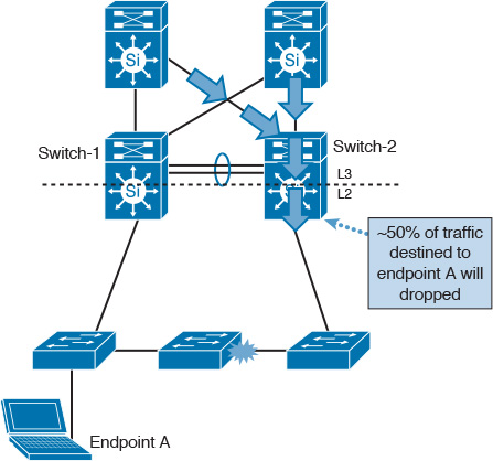
Layer 2 Design Model: Daisy-Chained Access Switches
Although this design model might be a viable option to overcome some limitations, network designers commonly use it as an interim solution. This design can introduce undesirable network behaviors. For instance, the design shown in Figure 2-6 can introduce the following issues during a link or node failure:
![]() Dual active HSRP
Dual active HSRP
![]() Possibility of 50 percent loss of the returning traffic for devices that still use the distribution switch-1 as the active Layer 3 FHRP gateway
Possibility of 50 percent loss of the returning traffic for devices that still use the distribution switch-1 as the active Layer 3 FHRP gateway
When suggesting an alternative solution to overcome a given design issue or limitation, it is important to make sure that the suggested design option will not introduce new challenges or issues during certain failure scenarios. Otherwise, the newly introduced issues will outweigh the benefits of the suggested solution.
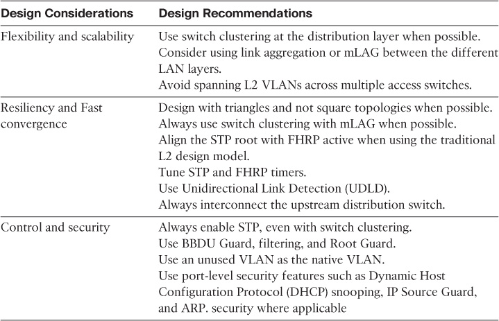
Layer 2 LAN Design Recommendations
Table 2-2 summarizes the different Layer 2 LAN design considerations and the relevant design recommendations.
Enterprise Layer 3 Routing Design Considerations
This section covers the various routing design considerations and optimization concepts that pertain to enterprise-grade routed networks.
IP Routing and Forwarding Concept Review
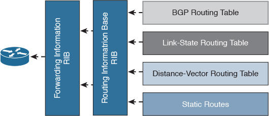
The main goal of routing protocols is to serve as a delivery mechanism to route packets to reach their intended destination. The end-to-end process of packets routing across the routed network is facilitated and driven by the concept of distributed databases. This concept is typically based on having a database of IP addresses (typically IPs of hosts and networks) on each Layer 3 node in the packet’s path, along with the next-hop IP addresses of the Layer 3 nodes that can be used to reach each of these IP addresses. This database is known as the Routing Information Database (RIB). In contrast, the Forwarding Information Base (FIB), also known as the forwarding table, contains the destination addresses and the interfaces required to reach those destinations, as depicted in Figure 2-7. In general, routing protocols are classified as either link-state, path-vector, or distance-vector protocols. This classification is based on how the mechanism of the routing protocol constructs and updates its routing table, and how it computes and selects the desired path to reach the intended IP destination.2
2. IETF draft: (Routing Information Base Info Model “draft-nitinb-i2rs-rib-info-model-02”)
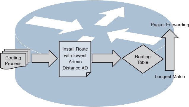
As illustrated in Figure 2-8, the typical basic forwarding decision in a router is based on three processes:
![]() Routing protocols
Routing protocols
![]() Routing table
Routing table
![]() Forwarding decision (switches packets)
Forwarding decision (switches packets)
Link-State Routing Protocol Design Considerations
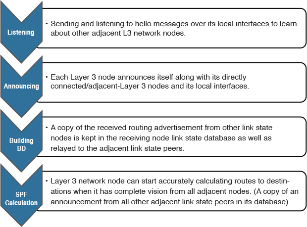
Open Shortest Path First (OSPF) and Intermediate System-to-Intermediate System (IS-IS) protocols as link-state routing protocols have a common conceptual characteristic in the way they build, interact, and handle L3 routing to some extent. Figure 2-9 illustrates the process of building and updating a link-state database (LSDB).
It is important to remember that although OSPF and IS-IS as link-state routing protocols are highly similar in the way they build the LSDB and operate, they are not identical! This section discusses the implications of applying link-state routing protocols (OSPF and IS-IS) on different network topologies, along with different design considerations and recommendations.
Link-State over Hub-and-Spoke Topology
In general, some implications should be considered when link-state routing protocols are applied on a hub-and-spoke topology, including the following:
![]() There is a concern with regard to scaling to a large number of spokes, because each spoke node typically will receive all other spoke nodes’ link-state information, because there is no effective means to control the distribution of routing information among these spokes.
There is a concern with regard to scaling to a large number of spokes, because each spoke node typically will receive all other spoke nodes’ link-state information, because there is no effective means to control the distribution of routing information among these spokes.
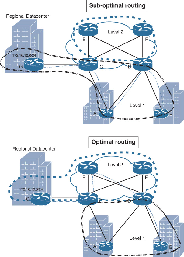
![]() Special consideration must be taken to avoid suboptimal routing, in which traffic can use remote sites (spokes) as a transit site to reach the hub or other spokes.
Special consideration must be taken to avoid suboptimal routing, in which traffic can use remote sites (spokes) as a transit site to reach the hub or other spokes.
For instance, summarization of routing flooding domains in a multi-area/flooding domain design with multiple border routers requires specific routing information between the border routers (Area Border Routers [ABRs] in OSPF or L1/L2 in IS-IS) over a nonsummarized link, to avoid using spoke sites as a transit path, as illustrated in Figure 2-10 [13].
So, for each hub-and-spoke flooding domain to be added to the hub routers, you need to consider an additional link between the hub routers in that domain. This is a typical use case scenario to avoid suboptimal routing with link-state routing protocols. However, when the number of flooding domains (for example, OSPF areas) increases, the number of VLANs, subinterfaces, or physical interfaces between the border routers will grow as well, which will result in scalability and complexity concerns. One of the possible solutions is to have a single link with adjacencies in multiple areas. (RFC 5185) [13]. For instance, in the scenario illustrated in Figure 2-11, there is a hub-and-spoke topology that uses OSPF multi-area design.
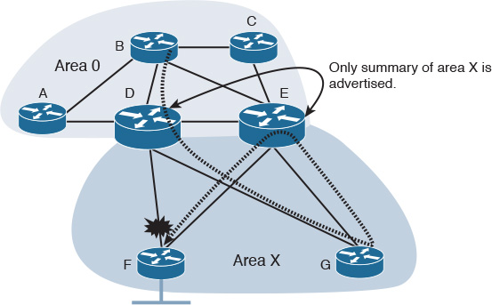
If the link between router D and router F (part of OSPF area X) fails, any traffic from router B destined to the LAN connected to router F going toward the summary advertised route by router D will traverse across the more specific route over the path G, E, then F.
To optimize this design during this failure scenario, there are multiple possible solutions, and here network designers must decide which solution is the most suitable one with regard to other design requirements such as application requirements where delay could affect critical business applications:
![]() Place the inter-ABR link (D to E) in area X (simple and provide “north to south” optimal routing in this topology).
Place the inter-ABR link (D to E) in area X (simple and provide “north to south” optimal routing in this topology).
![]() Place each spoke in its own area with link-state advertisement (LSA) type 3 filtering. (May lead to complex operations and limited scalability; “depends on the network size.”)
Place each spoke in its own area with link-state advertisement (LSA) type 3 filtering. (May lead to complex operations and limited scalability; “depends on the network size.”)
![]() Disable route summarization at the ABRs; for example advertise more specific routes from ABR router E. (May not always be desirable because this means reduced scalability and the loss of some of the value of the OSPF multi-area design.)
Disable route summarization at the ABRs; for example advertise more specific routes from ABR router E. (May not always be desirable because this means reduced scalability and the loss of some of the value of the OSPF multi-area design.)
Note
The link between the two hub nodes (for example, ABRs) will introduce the potential of a single point of failure to the design. Therefore, link redundancy (availability) between the ABRs may need to be considered.
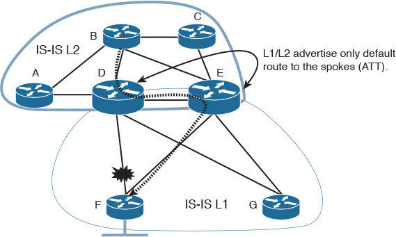
If IS-IS is applied to the topology in Figure 2-11 instead, using a similar setup where IS-IS L2 is to be used instead of the area 0 and IS-IS L1 is to be used by the spokes, the simplest way to optimize this architecture is to put the links between the border routers in IS-IS L1-L2 (overlapping levels capability), where we can extend L1 to overlap with L2 on the border router (ABR in OSPF), as illustrated in Figure 2-12. This will result in a topology that can support summarization with more optimal routing with regard to the failure scenario discussed above.
OSPF is a more widely deployed and proven link-state routing protocol in enterprise networks compared to IS-IS, especially with regard to hub-and-spoke topologies. IS-IS has limitations when it works on nonbroadcast multiple access (NBMA) multipoint networks.
OSPF Interface Network Type Considerations in a Hub-and-Spoke Topology
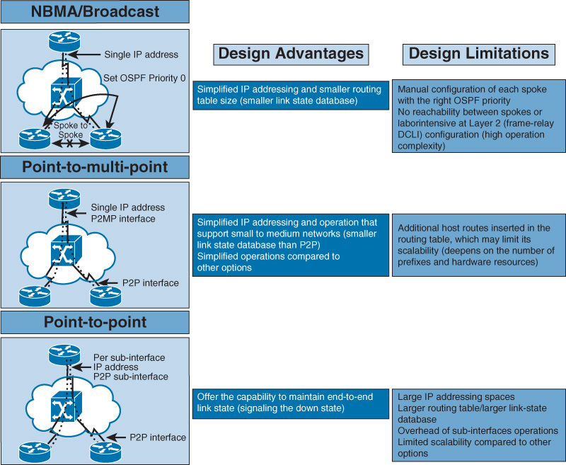
Figure 2-13 summarizes the different possible types of OSPF interfaces in a hub-and-spoke topology over NBMA transport (typically either Frame Relay or ATM), along with the associated design advantages and implications of each [13].
Link-State over Full-Mesh Topology
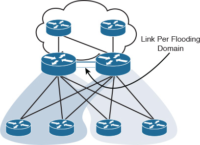
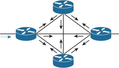
Fully meshed networks can offer a high level of redundancy and the shortest paths. However, the substantial amount of routing information flooding across a fully meshed network is a significant concern. This concern stems from the fact that each router will receive at least one copy of every new piece of information from each neighbor on the full mesh. For example, in Figure 2-14, each router has four adjacencies. When a router’s link connect to the LAN side fails, it must flood its LSA/LSP to each of the four neighbors. Each neighbor will then flood this LSA/LSP (link-state package) again to its neighbors. This process will culminate in a process like a broadcast being sent, due to this full-mesh connectivity and reflooding [13].
With link-state routing protocols, you can use the mesh group technique to reduce link-state information flooding in a full-meshed topology [23]. However, with link-state routing protocols in failure scenarios over a meshed topology, some routers may know about the failure before others within the mesh. This will typically lead to a temporarily inconsistent LSDB across the nodes within the network, which can result in transient forwarding loops. Even though the concept of a loop-free alternate (LFA) route can be considered to overcome situations like this, using LFA over a mesh topology will add complexity to the control plane.
Note
Later in this chapter, in the section “Hiding Topology and Reachability Information,” more details are provided about flooding domain and route summarization design considerations for link-state routing protocols, which can reduce the level of control plane complexity and optimize link-state information flooding and performance.
Note
Other mechanisms help to optimize and reduce link-state LSA/LSP flooding by reducing the transmission of subsequent LSAs/LSPs, such as OSPF flood reduction (described in RFC 4136). This is done by eliminating the periodic refresh of unchanged LSAs, which can be useful in fully meshed topologies
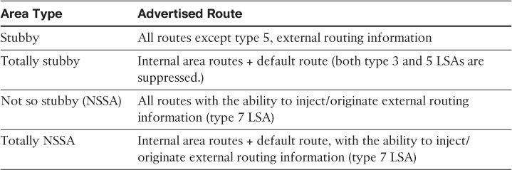
OSPF Area Types
Table 2-3 contains a summarized review of the different types of OSPF areas [21, 22].
Each of the OSPF areas allows certain types of LSAs to be flooded, which can be used to optimize and control route propagation across OSPF routed domain. However, if OSPF areas are not properly designed and aligned with other requirements, such as application requirements, it can lead to serious issues because of the traffic black-holing and suboptimal routing that can appear as a result to this type of design. Subsequent sections in this book discuss these points in more detail.
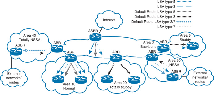
Figure 2-15 shows a conceptual high-level view of the route propagation, along with the different OSPF LSAs, in an OSPF multi-area design with different area types.
The typical design question is this: Where can these areas be used and why?
The basic standard answer is this: It depends on the requirements and topology.
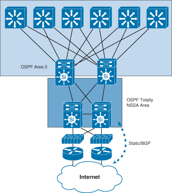
For instance, if no requirement specifies which path a route must take to reach external networks such as an extranet or the Internet, you can use the “totally NSSA” area type to simplify the design. For example, the scenario in Figure 2-16 is one of the most common design models that use OSPF NSSA. In this design model, the border area that interconnects the campus or data center network with the WAN or Internet edge devices can be deployed as totally NSSA. This deployment assumes that no requirement dictates which path should be used [15]. Furthermore, in the case of NSSA and multiple ABRs, OSPF selects one ABR to perform the translation from LSA type 7 to LSA type 5 and flood it into area 0 (normally the router with the highest router ID, as described in RFC 1587). This behavior can affect the design if the optimal path is required.
Note
RFC 3101 introduced the ability to have multiple ABRs perform the translation from LSA type 7 to type 5. However, the extra unnecessary number of LSA type 7 to type 5 translators may significantly increase the size of the OSPF LSDB. This can affect the overall OSPF performance and convergence time in large-scale networks with a large number of prefixes [RFC 3101].
Similarly, in the scenario depicted on the left in Figure 2-17, a data center in London hosts two networks (10.1.1.0/24 and 10.2.1.0/24). Both WAN/MAN links to this data center have the same bandwidth and cost. Based on this setup, the traffic coming from the Sydney branch toward network 10.2.1.0/24 can take any path. If this is not compromising any requirement (in other words, suboptimal routing is not an issue), the OSPF area 10 can be deployed as a “totally stubby area” to enhance the performance and stability of remote site routers.
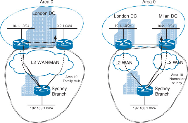
In contrast, the scenario on the right side of Figure 2-17 has a slightly different setup. The data centers are located in different geographic locations with a data center interconnect (DCI) link. In a scenario like this, the optimal path to reach the destination network can be critical, and using a totally stubby area can break the optimal path requirement. To overcome this limitation, there are two simple alternatives to use: either “normal OSPF area” or the “stubby area” for area 10. This ensures that the most specific route (LSA type 3) is propagated to the Sydney branch router to select the direct optimal path rather than crossing the international DCI [13].
In a nutshell, the goal of these types of different OSPF areas is to add more optimization to the OSPF multi-area design by reducing the size of the routing table and lowering the overall control plane complexity by reducing the size of the fault domains (link-state flooding domains). This size reduction can help to reduce overhead of the routers’ resources, such as CPU and memory. Furthermore, the reduction of the flooding domains’ size will help accelerate the overall network recovery time in the event of a link or node failure. However, in some scenarios where an optimal path is important, take care when choosing between these various area types.
In the scenarios illustrated in Figure 2-16 and Figure 2-17, asymmetrical routing is a possibility, which may be an issue if there are any stateful or stateless network devices in the path such as a firewall. However, this section focuses only on the concept of area design. Later in this book, you will learn how to manage asymmetrical routing at the network edge.
OSPF Versus IS-IS
It is obvious that OSPF and IS-IS as link-state routing protocols are similar and can achieve (to a large extent) the same result for enterprises in terms of design, performance, and limitations. However, OSPF is more commonly used by enterprises as the interior gateway protocol (IGP), for the following reasons:
![]() OSPF can offer a more structured and organized routing design for modular enterprise networks.
OSPF can offer a more structured and organized routing design for modular enterprise networks.
![]() OSPF is more flexible over hub-and-spoke topology with multipoint interfaces at the hub.
OSPF is more flexible over hub-and-spoke topology with multipoint interfaces at the hub.
![]() OSPF naturally runs over IP, which makes it a suitable option to be used over IP tunneling protocols such as generic routing encapsulation (GRE) and dynamic multipoint virtual private network (DMVPN), whereas with IS-IS, this is not a supported design.
OSPF naturally runs over IP, which makes it a suitable option to be used over IP tunneling protocols such as generic routing encapsulation (GRE) and dynamic multipoint virtual private network (DMVPN), whereas with IS-IS, this is not a supported design.
![]() In terms of staff knowledge and experience, OSPF is more widely deployed on enterprise-grade networks. Therefore, compared to IS-IS, more people have knowledge and expertise.
In terms of staff knowledge and experience, OSPF is more widely deployed on enterprise-grade networks. Therefore, compared to IS-IS, more people have knowledge and expertise.
However, if there is no technical barrier, both OSPF and IS-IS are valid options to consider.
Note
Some Cisco platforms and software versions do support IS-IS over GRE.3
3. “Cisco IOS XR Routing Configuration Guide for the Cisco CRS Router, Release 4.2.x,” http://www.cisco.com
Further Reading
OSPF Version 2, RFC 1247: http://www.ietf.org
OSPF for IPv6, RFC 2740: http://www.ietf.org
Domain-Wide Prefix Distribution with Two-Level IS-IS, RFC 5302: http://www.ietf.org
“OSPF Design Guide”: http://www.cisco.com
“How Does OSPF Generate Default Routes?”: http://www.cisco.com
“What Are OSPF Areas and Virtual Links?”: http://www.cisco.com
“OSPF Not So Stubby Area Type 7 to Type 5 Link-State Advertisement Conversion”: http://www.cisco.com
“IS-IS Network Types and Frame Relay Interfaces”: http://www.cisco.com
EIGRP Design Considerations
Enhanced Interior Gateway Routing Protocol (EIGRP) is an enhanced distance-vector protocol, relying on the Diffusing Update Algorithm (DUAL) to calculate the shortest path to a network. EIGRP, as a unique Cisco innovation, became highly valued for its ease of deployment, flexibility, and fast convergence. For these reasons, EIGRP is commonly considered by many large enterprises as the preferred IGP. EIGRP maintains all the advantages of distance-vector protocols while avoiding the concurrent disadvantages [16]. For instance, EIGRP does not transmit the entire routing information that exists in the routing table following an update event; instead, only the “delta” of the routing information will be transmitted since the last topology update. EIGRP is deployed in many enterprises as the routing protocol, for the following reasons:
![]() Easy to design, deploy, and support
Easy to design, deploy, and support
![]() Easier to learn
Easier to learn
![]() Flexible design options
Flexible design options
![]() Lower operational complexities
Lower operational complexities
![]() Fast convergence (subsecond)
Fast convergence (subsecond)
![]() Can be simple for small networks while at the same time scalable for large networks
Can be simple for small networks while at the same time scalable for large networks
![]() Supports flexible and scalable multi-tire campus and hub-and-spoke WAN design models
Supports flexible and scalable multi-tire campus and hub-and-spoke WAN design models
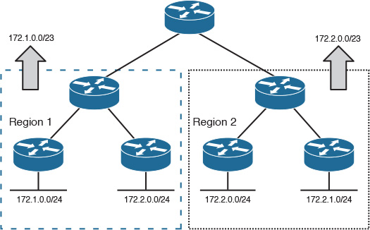
Unlike link-state routing protocols, such as OSPF, EIGRP has no hard edges. This is a key design advantage because hierarchy in EIGRP is created through routes summarization or routes filtering rather than relying on a protocol-defined boundary, such as OSPF areas. As illustrated in Figure 2-18, the depth of hierarchy depends on where the summarization or filtering boundary is applied. This makes EIGRP flexible in networks structured as a multitier architecture [19].
EIGRP: Hub and Spoke
As discussed earlier, link-state routing protocols have some scaling limitations when applied on a hub-and-spoke topology. In contrast, EIGRP offers more flexible and scalable capabilities for the hub-and-spoke types of topologies. One of the main concerns in a hub-and-spoke topology is the possibility of a spoke or remote site being used as a transit path due to a configuration error or a link failure. With link-state routing protocols, several techniques to mitigate this type of issue were highlighted. However, there are still scalability limitations associated with it.
However, EIGRP offers the capability to mark the remote site (spoke) as a stub, which is unlike the OSPF stub (where all routers in the same stub area can exchange routes and propagate failure and update information). With EIGRP, when the spokes are configured as a stub, it will signal to the hub router that the paths through the spokes should not be used as transit paths. As a result, there will be significant optimization to the design. This optimization results from the decrease in EIGRP query scope and the reduction of the unnecessary overhead associated with responding to queries by the spoke routers (for example, EIGRP stuck-in-active [SIA] queries) [19].
In Figure 2-19, router B will see it has only one path to the LAN connected to router A, rather than four paths.
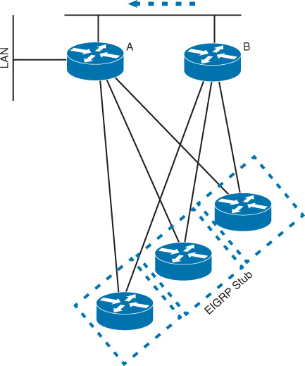
Consequently, enabling EIGRP Stub over a “hub-and-spoke” topology helps to reduce the overall control plane complexity as well as increases the scalability of the design to support large number of spokes without affecting its performance.
Note
With EIGRP, you can control what a stub router can advertise, such as directly connected links or redistributed static route. Therefore, network operators have more flexibility to control what is announced by the “stub” remote sites.
EIGRP Stub Route Leaking: Hub-and-Spoke Topology
You might encounter some scenarios like the one depicted in Figure 2-20, which is an extension to the EGRP stub design with a backdoor link between two remote sites. In this scenario, the HQ site is connected to the two remote sites over an L2 WAN. These remote sites are also interconnected directly via a backdoor link. Remote sites are configured as EIGRP stubs to optimize the remote sites’ EIGRP performance over the WAN.
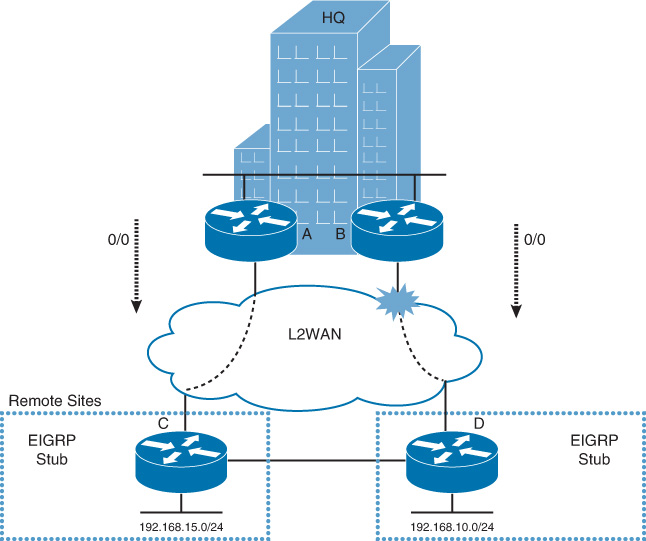
The issue with the design in this scenario is that if the link between router B and router D fails, the following will result as a consequence of this single failure:
![]() Router A cannot reach network 192.168.10.0/24 because router D is configured as a stub. Also, router C is a stub, which will not advertise this network to router A anyway.
Router A cannot reach network 192.168.10.0/24 because router D is configured as a stub. Also, router C is a stub, which will not advertise this network to router A anyway.
![]() Router D will not be able to receive the default from router A because router C is a stub as well.
Router D will not be able to receive the default from router A because router C is a stub as well.
This means that the remote site connected to router D will be completely isolated, without taking any advantage of the backdoor link. To overcome this issue, EIGRP offers a useful feature called stub leaking, where both routers D and C in this scenario can advertise routes to each other selectively, even if they are configured as a stub. Route filtering might need to be incorporated in scenarios like this, when an EIGRP leak map is introduced into the design to avoid any potential suboptimal routing that might happen as a consequence of routes leaking.
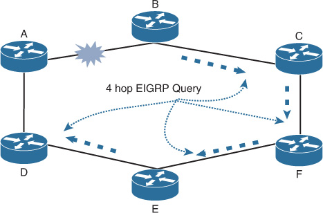
EIGRP: Ring Topology
Unlike link-state routing protocols, EIGRP has limitations with a ring topology. As depicted in Figure 2-21, the greater the number of nodes in the ring, the greater the number of queries to be sent during a link failure. As a general recommendation with EIGRP, always try to design in triangles where possible, rather than rings [20].
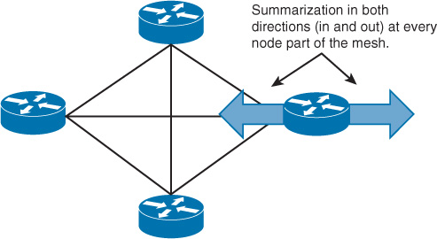
EIGRP: Full-Mesh Topology
EIGRP in a full-mesh topology (see Figure 2-22) is less desirable in comparison with link-state protocols. For example, with link-state protocols such as OSPF, network designers can designate one router to flood into the mesh and block flooding on the other routers, which can improve the topology. In contrast, with EIGRP, this capability is not available. The only way to mitigate the information flooding in an EIGRP mesh topology is by relying on route summarization and filtering techniques [19]. To optimize EIGRP in a mesh topology, the summarization must be into and out of the meshed network.
As discussed earlier, link state can lead to transient forwarding loops in ring and mesh topologies after a network component failure event. Therefore, both EIGRP and link state have limitations on these topologies, with different indications (fast and large number of EIGRP queries versus link-state transient loop).
EIGRP Route Propagation Considerations
EIGRP offers a high level of flexibility to network designers, which can fit different types of designs and topologies. However, like any other protocol, some limitations apply (especially with regard to route propagation) and may influence the design choices. Therefore, network designers must consider the following factors to avoid impacting the propagation of routing information, which can result in instable design:
![]() EIGRP bandwidth: By default, EIGRP is designed to use up to 50 percent of the main interface bandwidth for EIGRP packets; however, this value is configurable. The limitation with this concept occurs when there is a dialer or point-to-multipoint physical interface with several peers over one multipoint interface. In this scenario, EIGRP considers the bandwidth value on the main interface divided by the number of EIGRP peers on that interface to calculate the amount of bandwidth per peer. Consequently, when more peers are added over this multipoint interface, EIGRP will reach a point where it will not have enough bandwidth to operate over that dialer or multipoint interface appropriately. In addition, one of the common mistakes with regard to EIGRP and interface bandwidth is that sometimes network operators try to “influence” a best path selection decision in EIGRP DUAL by only tuning the bandwidth over an interface where the interface with the lowest bandwidth will be the least preferred. However, this approach can impact the EIGRP control plane peering functionality and scalability if it is tuned to a low value without proper planning.
EIGRP bandwidth: By default, EIGRP is designed to use up to 50 percent of the main interface bandwidth for EIGRP packets; however, this value is configurable. The limitation with this concept occurs when there is a dialer or point-to-multipoint physical interface with several peers over one multipoint interface. In this scenario, EIGRP considers the bandwidth value on the main interface divided by the number of EIGRP peers on that interface to calculate the amount of bandwidth per peer. Consequently, when more peers are added over this multipoint interface, EIGRP will reach a point where it will not have enough bandwidth to operate over that dialer or multipoint interface appropriately. In addition, one of the common mistakes with regard to EIGRP and interface bandwidth is that sometimes network operators try to “influence” a best path selection decision in EIGRP DUAL by only tuning the bandwidth over an interface where the interface with the lowest bandwidth will be the least preferred. However, this approach can impact the EIGRP control plane peering functionality and scalability if it is tuned to a low value without proper planning.
Therefore, the network designer must take this point into consideration and adopt alternatives, such as point-to-point subinterfaces under the multipoint interface. In addition, with overlay multipoint tunnel interfaces such as DMVPN the bandwidth may be required to be defined manually at the tunnel interface when there is a large number of remote spokes.
![]() Zero successor routes: When EIGRP tries to install routes in the RIB table and it is rejected, this is called zero successor routes because this route simply will not be propagated to other EIGRP neighbors in the network. This behavior typically happens due to one of the following two primary reasons:
Zero successor routes: When EIGRP tries to install routes in the RIB table and it is rejected, this is called zero successor routes because this route simply will not be propagated to other EIGRP neighbors in the network. This behavior typically happens due to one of the following two primary reasons:
![]() There is already the same route in the RIB table with a better administrative distance (AD).
There is already the same route in the RIB table with a better administrative distance (AD).
![]() When there are multiple EIGRP autonomous systems (AS) defined on the same router, the router will typically install any given route learned via both EIGRP autonomous systems with the same AD from one EIGRP AS, while the other will be rejected. Consequently, the route of the other EIGRP AS will not be propagated within its domain.
When there are multiple EIGRP autonomous systems (AS) defined on the same router, the router will typically install any given route learned via both EIGRP autonomous systems with the same AD from one EIGRP AS, while the other will be rejected. Consequently, the route of the other EIGRP AS will not be propagated within its domain.
Further Reading
savage-eigrp-xx, IETF draft, http://www.ietf.org
“Introduction to EIGRP,” http://www.cisco.com
“Configuration Notes for the Implementation of EIGRP over Frame Relay and Low Speed Links,” http://www.cisco.com
“What Does the EIGRP DUAL-3-SIA Error Message Mean?” http://www.cisco.com
Hiding Topology and Reachability Information Design Considerations
Technically, both topology and reachability information hiding can help to improve routing convergence time during a link or node failure. Topology and reachability information hiding also reduces control plane complexity and enhances network stability to a large extent. For example, if there is a link flapping in a remote site, this might cause all other remote sites to receive and process the update information every time this link flaps, which leads to instability and increased CPU processing.
However, to produce a successful design, the design must first align with the business goals and requirements (and not just be based on the technical drivers). Therefore, before deciding how to structure IGP flooding domains, network architects or designers must first identify the business’s goals, priorities, and drivers. Consider, for example, an organization that plans to merge with one of its business partners but with no budget allocated to upgrade any of the existing network nodes. When these two networks merge, the size of the network may increase significantly in a short period of time. As a result, the number of prefixes and network topology information will increase significantly, which will require more hardware resources such as memory or CPU.
Given that this business has no budget allocated for any network upgrade, in this case introducing topology and reachability information hiding to this network can optimize the overall network performance, stability, and convergence time. This will ultimately enable the business to meet its goal without adding any additional cost. In other words, the restructuring of IGP flooding domain design in this particular scenario is a strategic business-enabler solution.
However, in some situations, hiding topology and reachability information may lead to undesirable behaviors, such as suboptimal routing. Therefore, network designers must identify and measure the benefits and consequences by following the top-down approach. The following are some of the common questions that need to be thought about during the planning phase of the IGP flooding domain design:
![]() What are the business goals, priorities, and directions?
What are the business goals, priorities, and directions?
![]() How many Layer 3 nodes are in the network?
How many Layer 3 nodes are in the network?
![]() What is the number of prefixes?
What is the number of prefixes?
![]() Are there any hardware limitations (memory, CPU)?
Are there any hardware limitations (memory, CPU)?
![]() Is optimal routing a requirement?
Is optimal routing a requirement?
![]() Is low convergence time required?
Is low convergence time required?
![]() What IGP is used, and what is the used underlying topology?
What IGP is used, and what is the used underlying topology?
Furthermore, it is important that network designers understand how each protocol interacts with topology information and how each calculates its path, so as to be able to identify design limitations and provide valid optimization recommendations.
Link-state routing protocols take the full topology of the link-state routed network into account when calculating a path [18]. For instance, in the network illustrated in Figure 2-23, the router of remote site A can reach the HQ network (192.168.1.0/24) through the WAN hub router. Normally, if the link between the WAN hub router and router A in the WAN core fails, remote site A will be notified about this topology change “in a flat link-state design.” In fact, in any case, the remote site A router will continue to route its traffic via the WAN hub router to reach the HQ LAN 192.168.1.0/24.
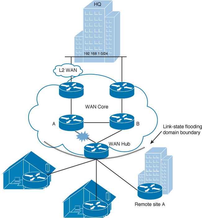
In other words, in this scenario, the link failure notifications between the WAN hub router and the remote site routers are considered as unnecessary extra processing for the remote site routers. This extra processing could lead to other limitations in large networks with a large number of prefixes and nodes, such as network and CPU spikes. In addition, the increased size of the LSDB will impact routing calculation and router memory consumption [8]. Therefore, by introducing the principle of “topology hiding boundary” at the WAN hub router (for example, by using OSPF multi-area design), the overall routing design will be optimized (different fault domains) in terms of performance and stability.
A path-vector routing protocol (Border Gateway Protocol [BGP]) can achieve topology hiding by simply using either route summarization or filtering, and distance-vector protocols, by nature, do not propagate topology information. Moreover, with route summarization, network designers can achieve “reachability information hiding” for all the different routing protocols [19].
Note
Link state can offer built-in information hiding capabilities (route suppression) by using different type of flooding domains, such as L1/L2 in IS-IS and stubby types of areas in OSPF.
The subsequent sections examine where and why to break a routed network into multiple logical domains. You will also learn summarization techniques and some of the associated implications that you need to consider.
Note
Although route filtering can be considered as an option for hiding reachability information, it is often somewhat complicated with link-state protocols.
IGP Flooding Domains Design Considerations
As discussed earlier, modularity can add significant benefit to the overall network architecture. By applying this concept to the design of logical routing architectural domains, we can have a more manageable, scalable, and flexible design. To achieve this, we need to break a flat routing design into one that is more hierarchical and has modularity in its overall architecture. In this scenario, we may have to ask the following questions: How many layers should we consider in our design? How many modules or domains is good practice?
The simple answer to these questions depends on several factors, including the following:
![]() Design goal (simplicity versus scalability versus stability)
Design goal (simplicity versus scalability versus stability)
![]() Network topology
Network topology
![]() Network size (nodes, routes)
Network size (nodes, routes)
![]() Routing protocol
Routing protocol
![]() Network type (for example, enterprise versus service provider)
Network type (for example, enterprise versus service provider)
The following sections covers the various design considerations for IGP flooding domains, starting with a review of the structure of link-state and EIGRP domains.
Link-State Flooding Domain Structure
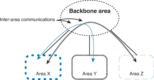
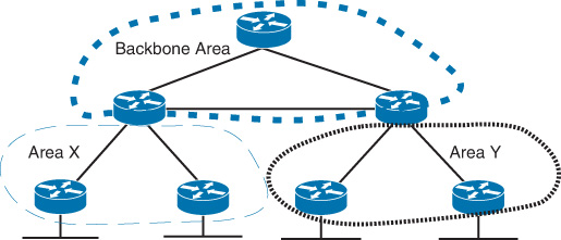
Both OSPF and IS-IS as link-state routing protocols can divide the network into multiple flooding domains, as discussed earlier in this book. Dividing a network into multiple flooding domains, however, requires an understanding of the principles each protocol uses to build and maintain communication between the different flooding domains. In a multiple flooding domain design with OSPF, a backbone area is required to maintain end-to-end communication between all other areas (regardless of its type). In other words, area 0 in OSFP is like the glue that interconnects all other areas within an OSPF domain [22]. In fact, nonbackbone OSPF areas and area 0 (backbone area) interconnect and communicate in a hub-and -spoke fashion, as illustrated in Figure 2-24.
Similarly, with IS-IS, its levels chain (IS-IS flooding domains) must not be disjointed (L2 to L1/L2 to L1 and vice versa) for IS-IS to maintain end-to-end communications, where the level 2 can be seen as analogous to area 0 in OSPF.
The natural communication behavior of link-state protocols across multiple flooding domains requires at least one router to be dually connected to the core flooding domain (backbone area) and the other area or areas, where an LSDB for each area is stored along with separate shortest path first (SPF) calculations for each area. Moreover, the characteristic of the communication between link-state flooding domains (between border routers) is like a distance-vector protocol. In OSPF terminology, this router is called the Area Border Router (ABR). In IS-IS, the L1/L2 router is analogous to the OSPF ABR.
In general, OSPF and IS-IS are two-layer hierarchy protocols; however, this does not mean that they cannot operate well in networks with more hierarchies (as discussed later in this section).
In addition, although both OSPF and IS-IS are suitable for two-layer hierarchy network architecture, there are some differences in the way that their logical layout (flooding domains such as areas, levels) can be designed. For example, OSPF has a hard edge at the flooding domain borders. Typically, this is where routing policies are applied, such as route summarization and filtering, as shown in Figure 2-25.
By contrast, IS-IS routing information of the different levels (L1 and L2) is (technically) carried over different packets. This helps IS-IS have a softer edge at its flooding domain borders. This makes it more flexible than OSPF, because the L2 routing domain can overlap with the L1 domains, as shown in Figure 2-26.
Consequently, IS-IS can perform better when optimal routing is required with multiple border routers, whereas OSPF requires special consideration with regards to the inter-ABR links (for example, which area to be part of, or in which direction is optimal routing more important).
Recommendation: With both OSPF and IS-IS, the design must always reflect that the backbone cannot be partitioned in case of a link or node failure. Although an OSPF virtual link can help to fix partitioned backbone area issues, it is not a recommended approach. Instead, redesign of the logical or physical architecture is highly desirable in this case. Nevertheless, an OSPF virtual link may be used as an interim solution (see the following example).
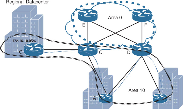
The scenario shown in Figure 2-27 illustrates poorly designed OSPF areas. It is considered a poor design because the OSPF backbone area has the potential to be partitioned if the direct interconnect link between the regional data centers (London and Sydney) fails. This will result in communication isolation between the London and Sydney data centers. However, let’s assume that this organization needs to use its regional HQs (Melbourne, Amsterdam, and Singapore), which are interconnected in a hub-and-spoke fashion, as a backup transit path when the link between the London and Sydney sites is down.
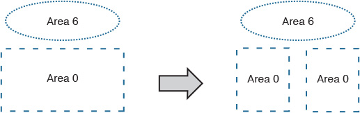
Based on the current OSPF area design, a nonbackbone area (area 6) cannot be used as a transit area. Figure 2-28 illustrates the logical view of OSPF areas before and after the failure event on the data center interconnect between London and Sydney data centers, which leads to a disjoint area 0 situation [22].
The ideal fix to this issue is to add redundant links from the London data center to WAN backbone router Y and/or from the Sydney data center to WAN backbone router X or to add a link between WAN backbone routers X and Y in area 0.
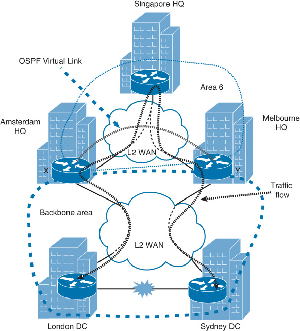
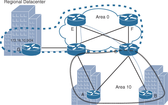
However, let’s assume that the provisioning of the links takes a while and this organization requires a quick fix to this issue. As shown in Figure 2-29, if you deploy an OSPF virtual link between WAN backbone routers X and Y in Amsterdam and Melbourne, respectively (across the hub site in Singapore), OSPF will consider this link as a point-to-point link. Both WAN backbone routers (ABRs) X and Y will form a virtual adjacency across this virtual link. As a result, this path can be used as an alternate path to maintain the communication between London and Sydney data centers when the direct link between them is down.
Note
The solution presented in this scenario is based on the assumption that traffic flowing over multiple international links is acceptable from the perspective of business and application requirements.
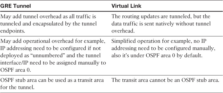
Note
You can use a GRE tunnel as an alternative method to the OSPF virtual link to fix issues like the one just described; however, there are some differences between using a GRE tunnel versus an OSPF virtual link, as summarized in Table 2-4.
Link-State Flooding Domains
One of the most common questions when designing OSPF or IS-IS is this: What is the maximum number of routers that can be placed within a single area?
The common rule of thumb specifies between 50 and 100 routers per area or IS-IS level. However, in reality it is hard to generalize the recommended maximum number of routers per area because the maximum number of routers can be influenced by a number of variables, such as the following:
![]() Hardware resources (such as memory, CPU)
Hardware resources (such as memory, CPU)
![]() Number of prefixes (can be influenced by routes’ summarization design)
Number of prefixes (can be influenced by routes’ summarization design)
![]() Number of adjacencies per shared segment
Number of adjacencies per shared segment
Note
The amount of available bandwidth with regard to the control plane traffic such as link-state LSAs/LSPs is sometimes a limiting factor. For instance, the most common quality of service (QoS) standard models followed by many organizations allocate one of the following percentages of the interface’s available bandwidth for control (routing) traffic:4 4-class model, 7 percent; 8-class model, 5 percent; and 12-class model, 2 percent. This is more of a concern when the interconnection is a low-speed link such as legacy WAN link (time-division multiplexing [TDM] based, Frame Relay, or ATM) with limited bandwidth. Therefore, other alternatives are sometimes considered with these types of interfaces, such as passive interface or static routing.
4. “Medianet WAN Aggregation QoS Design 4.0,” http://www.cisco.com
For instance, many service providers run tens of hundreds of routers within one IS-IS level. Although this may introduce other design limitations with regard to modern architectures, in practice it is proven as a doable design. In addition, today’s router capabilities, in terms of hardware resources, are much stronger and faster than routers that were used five to seven years ago. This can have a major influence on the design, as well, because these routers can handle a high number of routes and volume of processing without any noticeable performance degradation.
In addition, the number of areas per border router is also one of the primary considerations in designing link-state routing protocols, in particular OSPF. Traditionally, the main constraint with the limited number of areas per ABR is the hardware resources. With the next generation of routers, which offer significant hardware improvements, ABRs can hold a greater number of areas. However, network designers must understand that additional areas to be added per ABR correlates to potential lower expected performance (because the router will store a separate LSDB per area).
In other words, hardware capabilities of the ABR are the primary deterministic factor of the number of areas that can be allocated per ABR, considering the number of prefixes per area as well. Traditionally, the rule of thumb is to consider two to three areas (including backbone area) per ABR. This is a foundation and can be expanded if the design requires more areas per ABR, with the assumption that the hardware resources of the ABR can handle this increase.
In addition to these facts and variables, network designers should consider the nature of the network and the concept of fault isolation and design modularity for large networks that can be designed with multiple functional fault domains (modules). For example, large-scale routed networks are commonly divided based on the geographic location for global networks or based on an administrative domain structure if they are managed by different entities.
EIGRP Flooding Domains Structure
As discussed earlier, EIGRP has no protocol-specific flooding domains or structure. However, EIGRP with route summarization or filtering techniques can break the flooding domains into multiple hierarchies of routing domains, which can reduce the EIGRP query scope, as depicted in Figure 2-30. This concept is a vital contributor to the optimization for the overall EIGRP design in terms of scalability, simplicity, and convergence time. In addition, EIGRP offers a higher degree of flexibility and scalability in networks with three and more levels in their hierarchies as compared to link-state routing protocols [19].
Routing Domain Logical Separation
The two main drivers for breaking a routed network into multiple logical domains (fault domains) are the following: to improve the performance of the networks and routers (fault isolation), and to modularize the design (to make it become simpler, more stable and scalable). These two drivers enhance network convergence and increase the overall routing architecture scalability. Furthermore, breaking the routed topology into multiple logical domains will facilitate topology aggregation and information hiding. It is critical to decide where a routing domain can be divided into two or multiple logical domains. In fact, several variables influence the location where the routing domains are broken or divided. The considerations discussed in the sections that follow are the primary influencers that help to determine the correct location of the logical routing boundaries. Network designers need to consider these when designing or restructuring a routed network.
Underlying Physical Topology
As discussed in Chapter 1, “Network Design Requirements: Analysis and Design Principles,” the physical network layout is like the foundation of a building. As such, it is the main influencer when designing the logical structure of a routing domain (for example, a hub-and-spoke versus ring topology). For instance, the level of hierarchy held by a given network can impact the logical routing design if its structure includes two, three, or more tiers, as illustrated in Figure 2-31.
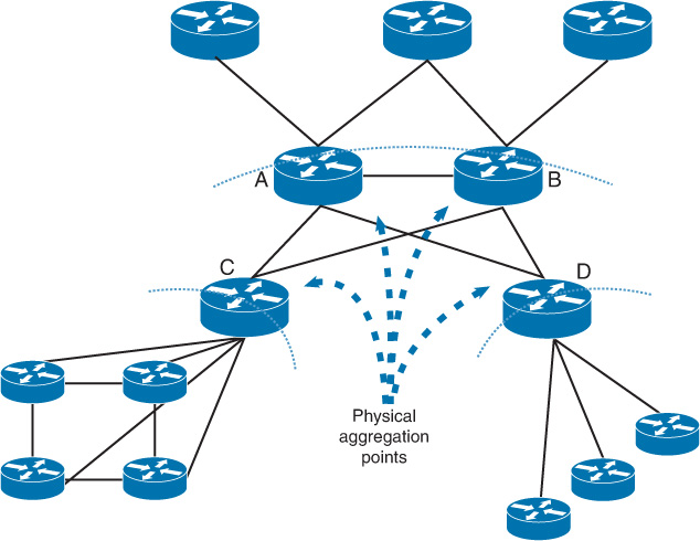
Moreover, the points in the network where the interconnections or devices meet (also known as chokepoints) at any given tier within the network are a good potential border location of a fault domain boundary, such as ABR in OSPF [19]. For instance, in Figure 2-32, the network is constructed of three-level hierarchies. Routers A and B and routers C and D are good potential points for breaking the routing domain (physical aggregation points). Also, these boundaries can be feasible places to perform route summarizations.
The other important factor with regard to the physical network layout is to break areas that have a high density of interconnections into separate logical fault domains where possible. As a result, devices in each fault domain will have smaller reachability databases (for example, LSDB) and will only compute paths within their fault domain, as illustrated in Figure 2-33. This will ultimately lead to the reduction of the overall control plane design complexity [8]. This concept will promote a design that can facilitate the support of other design principles, including simplicity, modularity, scalability, and topology and reachability information hiding.
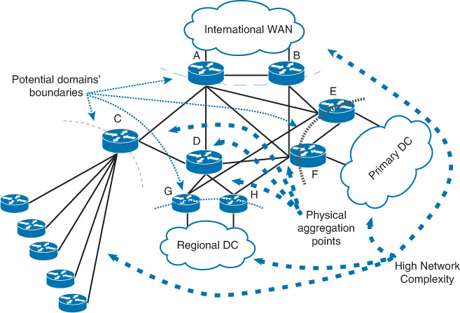
The network illustrated in Figure 2-33 has four different functional areas:
![]() The primary data center
The primary data center
![]() The regional data center
The regional data center
![]() The international WAN
The international WAN
![]() The hub-and-spoke network for some of the remote sites
The hub-and-spoke network for some of the remote sites
From the perspective of logical separation, you should place each one of the large parts of the network into its own logical domain. The logical topology can be broken using OSPF areas, IS-IS levels, or EIGRP route summarization. The question you might be asking is this: Why has the domain boundary been placed at routers G and H rather than router D? Technically, both are valid places to break the network into multiple logical domains. However, if we place the domain boundary at router D, both the primary data center network and regional data center will be under same logical fault domain. This means the network may be less scalable and associated with lower control plane stability because routers E and F will have a full view of the topology of the regional data center network connected to routers G and H. In addition, routers G and H most probably will face the same limitations as routers E and F. As a result, if there is any link flap or routing change in the regional data center network connected to router G or H, it will be propagated across to routers E and F (unnecessary extra load and processing).
Traffic Pattern and Volume
By understanding traffic pattern (for example, south-north versus east-west) and traffic volume trends, network designers can better understand the impact if a logical topology were to be divided into multiple domains on certain points (see Figure 2-34). For example, OSPF always prefers the path over the same area regardless of the link cost over other areas. (For more information about this, see the section “IGP Traffic Engineering and Path Selection: Summary.”) In some situations, this could lead to suboptimal routing, where a high volume of traffic will travel across low-capacity links or expensive links with strict billing that not every type of communications should go over it; this results from the poor design of OSPF areas, which did not consider bandwidth or cost requirements.
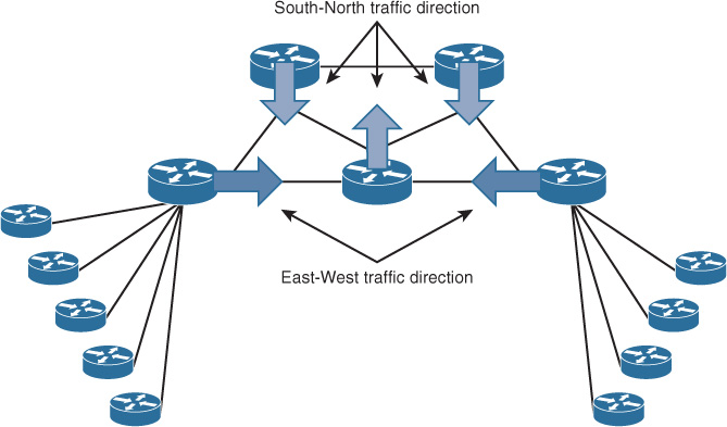
Similarly, if the traffic pattern is mostly north-south, such as in a hub-and-spoke topology where no communication between the spokes is required, this can help network designers to avoid placing the logical routing domain boundary at points likely to using spoke sites as transit sites (suboptimal routing). For instance, the scenario depicted in Figure 2-35 demonstrates how the application of the logical area boundaries on a network can influence the path selection. Traffic sourced from router B going to the regional data center behind router G should (optimally) go through router D, and then across one of the core routers E or F, and finally to router C to reach the data center over one of the core high-speed links. However, the traffic is currently traversing the low-speed link via router A. This path (B-D-A-C-G) is within the same area (area 10), as shown in Figure 2-35.
No route filtering or any type of summarization is applied to this network. This suboptimal routing results entirely from the poor design of OSPF areas. If you apply the concepts discussed in this section, you can optimize this design and fix the issue of suboptimal routing, as follows:
![]() First, the physical network is a three-tier hierarchy. Routers C and D are the points where the access, data center, and core links meet, which makes them a good potential location to be the area border (which is already in place).
First, the physical network is a three-tier hierarchy. Routers C and D are the points where the access, data center, and core links meet, which makes them a good potential location to be the area border (which is already in place).
![]() Second, if you divide this topology into functional domains, you can, for example, have three parts (core, remote sites, and data center), with each placed in its own area. This can simplify summarization and introduce modularity to the overall logical architecture.
Second, if you divide this topology into functional domains, you can, for example, have three parts (core, remote sites, and data center), with each placed in its own area. This can simplify summarization and introduce modularity to the overall logical architecture.
![]() The third point here is traffic pattern. It is obvious that there will be traffic from the remote sites to the regional data center, which needs to go over the high-speed links rather than going over the low-speed links by using other remote sites as a transit path.
The third point here is traffic pattern. It is obvious that there will be traffic from the remote sites to the regional data center, which needs to go over the high-speed links rather than going over the low-speed links by using other remote sites as a transit path.
Based on this analysis, the simple solution to this design is to either place the data center in its own area or to make the data center part of area 0, as illustrated in Figure 2-36, with area 0 extended to include the regional data center.
Note
Although both options are valid solutions, on the CCDE exam the correct choice will be based on the information and requirements provided. For instance, if one of the requirements is to achieve a more stable and modular design, a separate OSPF area for the regional data center will be the more feasible option in this case.
Similarly, if IS-IS is used in this scenario as illustrated in Figure 2-37, router B will always use router A as a transit path to reach the regional data center prefix. Over this path (B-D-A-C-G), the regional data center prefix behind router G will be seen as IS-IS level 1, and based on IS-IS route selection rules, this path will be preferred compared to the one over the core, in which it will be announced as an IS-IS level 2 route. (For more information about this, see the section “IGP Traffic Engineering and Path Selection: Summary.”) Figure 2-37 suggests a simple possible solution to optimize IS-IS flooding domain design (levels): including the regional data center as part of IS-IS level 2. This ensures that traffic from the spokes (router B in this example) destined to the regional data center will always traverse the core network rather transiting any other spoke’s network.
Route Summarization
The other major factor when deciding where to divide logical topology of a routed network is where summarization or reachability information hiding can take place. The important point here is that the physical layout of the topology must be taken into account. In other words, you cannot decide where to place the reachability information hiding boundary (summarization) without referring to what the physical architecture looks like and where the points are that can enhance the overall routing design if summarization is enabled. Subsequent sections in this chapter cover route summarization design considerations in more detail.
Security Control and Policy Compliance
This pertains more to what areas of a certain network have to be logically separated from other parts of the network. For example, an enterprise might have a research and development lab (R&D) where different types of unified communications applications are installed, including routers and switches. Furthermore, the enterprise security policy may dictate that this part of the network must be logically contained and only specific reachability information needs to be leaked between this R&D lab environment and the production network. Technically, this will lead to increased network stability and policy control.
Route Summarization
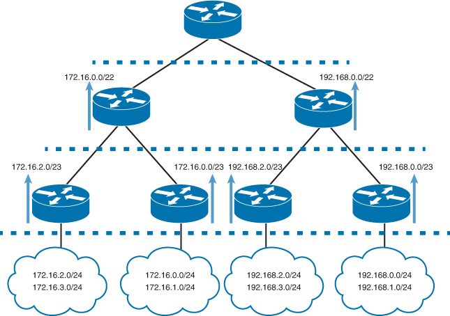
By having a well-structured IP address align with the physical layout with reachability information hiding using routes summarization, as shown in Figure 2-38, network designers can achieve an optimized level of network design simplicity, scalability, and stability.
For example, based on the routes’ summarization structure illustrated in Figure 2-38, if there is any link flap in a remote site in region 2, it will not affect the remote site routers of region 1 in processing or updating their topology database (which in some situations might cause unnecessary path recalculation and processing, which in turn may lead to service interruption). Usually, route summarization facilitates the reduction of the RIB table size by reducing the number of route counts. This means less memory, lower CPU utilization, and faster convergence time during a network change or following any failure event. In other words, the boundary of the route summarization almost always overlaps with the boundary of the fault domain.
However, not every network has a structured network IP addressing like the one shown in Figure 2-38. Therefore, network designers must consider alternatives to overcome this issue. In some situations, the solution is “not to summarize.” For instance, Figure 2-39 illustrates a network with unstructured IP addressing, and the business may not able to afford changing their IP scheme in the near future.
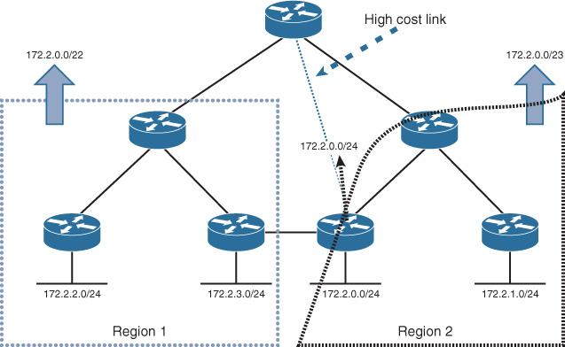
Moreover, in some scenarios, the unstructured physical connectivity can introduce challenges with route summarization. For example, in Figure 2-40, summarization can lead to forcing all the traffic from the hub site to always prefer the high-cost and low-bandwidth link to reach 172.2.0.0/24 network (more specific route over the high-cost nonsummarized link), which may lead to undesirable outcome from the business point of view (for example slow applications’ response time over this link).
As a general rule of thumb (not always), summarization should be considered at the routing logical domain boundaries. The reason why summarization might not always be considered at the logical boundary domain is because in some designs it can lead to suboptimal routing or traffic black-holing (also known as summary black holes). The following subsections discuses summary suboptimal routing and summary black-holing in more detail.
Summary Black Holes
The principle of route summarization is based on hiding specific reachability information. This principle can optimize many network designs, as discussed earlier; however, it can lead to traffic black-holing in some scenarios because of the specific hidden routing information. In the scenario illustrated in Figure 2-41, router A and B send the summary route only (172.1.0.0/21) with the same metric toward router C. Based on this design, in case of link failure between router D and E, the routing table of router C will remain intact, because it is receiving only the summary. Consequently, there is potential for traffic black-holing. For instance, traffic sourced from router C destined to network 172.1.1.0/24 landing at router B will be dropped because of this summarization black-holing. Moreover, the situation can become even worse if router C is performing per-packet load balancing across routers A and B. In this case, 50 percent of the traffic is expected to be dropped. Similarly, if router C is load balancing on a per-session basis, hypothetically some of the sessions will reach their destinations and others may fail. As a result, route summarization in this scenario can lead to a serious connectivity issues in some failure situations [18], [19].
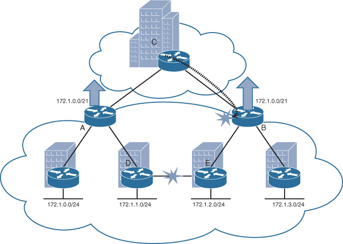
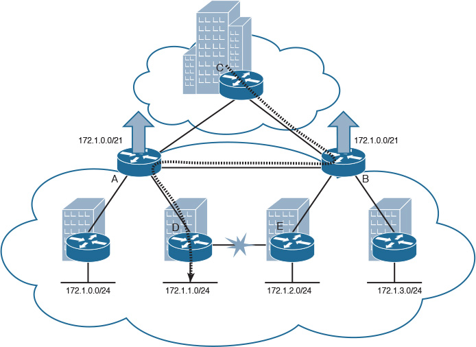
To mitigate this issue and enhance the design in Figure 2-41, summarization either should be avoided (this option might not be always desirable because it can reduce the stability and scalability in large networks) or at least one nonsummarized link must be added between the summarizing routers (in this scenario, between routers A and B, as illustrated in Figure 2-42). The nonsummarized link can be used as an alternate path to overcome the route summarization black-holing issue described previously.
Suboptimal Routing
Although hiding reachability information with route summarization can help to reduce control plane complexity, it can lead to suboptimal routing in some scenarios. This suboptimal routing, in turn, may lead traffic to use a lower-bandwidth link or an expensive link, over which the enterprise might not want to send every type of traffic. For example, if we use the same scenario discussed earlier in the OSPF areas, we then apply summarization on the data center edge routers of London and Milan and assume that the link between Sydney and Milan is a high-cost link that has a typically lower routing metric, as depicted in Figure 2-43.
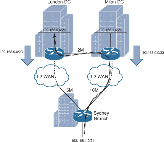
Note
The example in Figure 2-43 is “routing protocol” neutral. It can apply to all routing protocols in general.
As illustrated in Figure 2-43, the link between the Sydney branch and Milan data center is 10 Mbps, and the link to London is 5 Mbps. In addition, the data center interconnect between Milan and London data centers is only 2 Mbps. In this particular scenario, summarization toward the Sydney branch from both data centers will typically hide the more specific route. Therefore, the Sydney branch will send traffic destined to any of the data centers over the high-bandwidth link (with lower routing metric); in this case, the Sydney-Milan path will be preferred (almost always higher bandwidth = lower path metric). This behavior will cause suboptimal routing for traffic destined to London data center network. This suboptimal routing in turn can lead to an undesirable experience, because rather than having 5 Mbps between Sydney branch and London data center, their maximum bandwidth will be limited to the data center interconnect link capacity, which is 2 Mbps in this scenario. This is in addition to the extra cost and delay that will from the traffic having to traverse multiple international links.
Even so, this design limitation can be resolved via different techniques based on the use of the routing protocol, as summarized in Table 2-5.
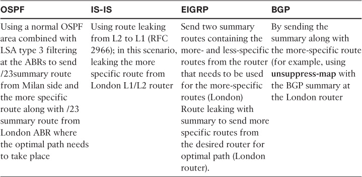
Figure 2-44 illustrates link-state areas/levels application with regard to the discussed scenario and the suggested solutions, because the different areas/levels designs can have a large influence on the overall traffic engineering and path selection.
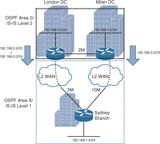
with IS-IS, L1-L2 (ABR) may send default route toward the L1 domain and the route leaking at the London ABR will leak/send the more specific local prefix for optimal routing.
Based on the these design considerations and scenarios, we can conclude that although route summarization can optimize the network design for the several reasons (discussed earlier in this chapter), in some scenarios summarization from the core networks toward the edge or remote sites can lead to suboptimal routing. In addition, summarization from the remote sites or edge routers toward the core network may lead to traffic black holes in some failure scenarios. Therefore, to provide a robust and resilient design, network designers must pay attention to the different failure scenarios when considering route summarization [19].
IGP Traffic Engineering and Path Selection: Summary
By understanding the variables that influence a routing protocol decision to select a certain path, network designers can gain more control to influence route preference over a given path based on a design goal. This process is also known as traffic engineering.
In general, routing protocols perform what is known as destination traffic engineering, where the path selection is always based on the targeted prefix and the attributes of the path to reach this prefix. However, each of the three IGPs discussed in this chapter has its own metrics, algorithm, and default preferences to select routes. From a routing point of view, they can be altered to control which path is preferred or selected over others, as summarized in the sections that follow.
OSPF
If multiple routes cover the same network with different types of routes, such as interarea (LSA type 3) or external (LSA type 5), OSPF considers the following list “in order” to select the preferred path (from highest preference to the lowest):
1. Intra-area routes
2. Inter-area routes
3. External type 1 routes
4. External type 2 routes
Let’s take a scenario where there are multiple routes covering the same network with the same route type as well; for instance, both are interarea route (LSA type 3). In this case, the OSPF metric (cost) that is driven by the links’ bandwidth is used as a tiebreaker to select the preferred path. Typically, the route with the lowest cost is chosen as the preferred path.
If multiple paths cover the same network with the same route type and cost, OSPF will typically select all the available paths to be installed in the routing table. Here, OSPF performs what is known as equal-cost multipath (ECMP) routing across multiple paths.
For external routes with multiple Autonomous System Border Routers (ASBRs), OSPF relies on LSA type 4 to describe the path’s cost to each ASBR that advertises the external routes. For instance, in case of multiple ASBRs advertising the same external OSPF E2 prefixes carrying the same redistributed metric value, the ASBR with the lowest reported forwarding metric (cost) will win as the preferred exit point.
IS-IS
Typically, with IS-IS, if multiple routes cover the same network (same exact subnet) with different route types, IS-IS follows the sequence here “in order” to select the preferred path:
1. Level 1
2. Level 2
3. Level 2 external with internal metric type
4. Level 1 external with external metric type
5. Level 2 external with external metric type
Like OSPF, if there are multiple paths to a network with the same exact subnet, route type, and cost, IS-IS selects all the available paths to be installed in the routing table (ECMP).
EIGRP
EIGRP has a set of variables that can solely or collectively influence which path a route can select. For more stability and simplicity, bandwidth and delay are commonly used for this purpose. Nonetheless, it is always simpler and safer to alter delay for EIGRP path selection, because of some implications associated with tuning bandwidth for EIGRP traffic engineering purposes discussed earlier in this chapter, which requires careful planning.
Like other IGPs, EIGRP supports the concept of ECMP; in addition, it does support “unequal cost load balancing,” as well, with proportional load sharing.
Summary of IGP Characteristics
As discussed in this chapter, each routing protocol behaves and handles routing differently on each topology. Table 2-6 summarizes the characteristics of the IGPs, taking into account the used topology.
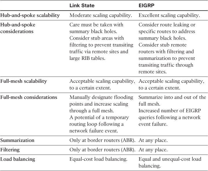
Note
As you’ll notice, the full mesh in the preceding table has no excellent scalability among the IGPs. This is because the nature of full-mesh topology is not very scalable. (The larger the mesh becomes, the more complicated the control plane will be.)
BGP Design Considerations
Border Gateway Protocol (BGP) is an Internet Engineering Task Force (IETF) standard, and the most scalable of all routing protocols. As such, BGP is considered as the routing protocol of the global Internet, as well as for service provider-grade networks. In addition, BGP is the desirable routing protocol of today’s large-scale enterprise networks because of its flexible and powerful attributes and capabilities. Unlike IGPs, BGP is used mainly to exchange network layer reachability information (NLRI) between routing domains. (The routing domain in BGP terms is referred to as an autonomous system (AS); typically, it is a logical entity with its own routing and policies, and is usually under same administrative control.) Therefore, BGP is almost always the preferred inter-AS routing protocol. The typical example is the global Internet, which is formed by numerous interconnected BGP autonomous systems.
There are two primary forms of BGP peering:
![]() Interior BGP (iBGP): The peering between BGP neighbors that is contained within one AS
Interior BGP (iBGP): The peering between BGP neighbors that is contained within one AS
![]() Exterior BGP (eBGP): The peering between BGP neighbors that occurs between the boundaries of different autonomous systems (interdomain)
Exterior BGP (eBGP): The peering between BGP neighbors that occurs between the boundaries of different autonomous systems (interdomain)
Interdomain Routing
Typically, the exterior gateway protocol (EGP) (eBGP) is mainly used to determine paths and route traffic between different autonomous systems; this function is known as interdomain routing. Unlike an IGP (where routing is usually performed based on protocol metrics to determine the desired path within an AS), EGP relies more on policies to route or interconnect two or more autonomous systems. The powerful policies of EGP allows it to ignore several attributes of routing information that typically an IGP takes into consideration. Therefore, an EGP can offer more simplified and flexible solutions to interconnect various autonomous systems based on predefined routing policies.
Table 2-7 summarizes common AS terminology with regard to interdomain routing concept and as illustrated in Figure 2-45.
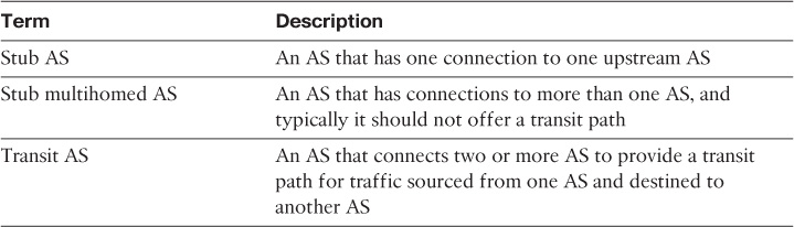
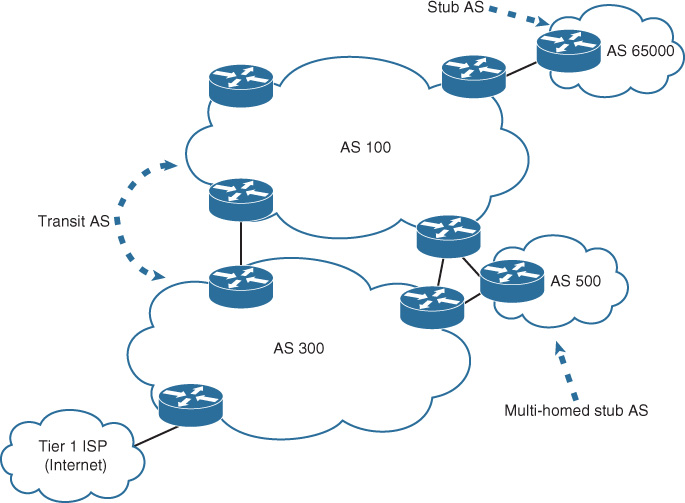
Furthermore, normally, each AS has its own characteristic in terms of administrative boundaries, geographic restrictions, QoS scheme, cost, and legal constraints. Therefore, for the routing policy control to deliver its value to the business with regard to these variables, there must be a high degree of flexibility in how and where the policy control can be imposed. Typically, there are three standard levels where interdomain routing control can be considered (inbound, transit, and outbound):
![]() Inbound interdomain routing policy to influence which path egress traffic should use to reach other domains
Inbound interdomain routing policy to influence which path egress traffic should use to reach other domains
![]() Outbound interdomain routing policy to influence which path ingress traffic sourced from other domains should use to reach the intended destination prefixes within the local domain
Outbound interdomain routing policy to influence which path ingress traffic sourced from other domains should use to reach the intended destination prefixes within the local domain
![]() Transportation interdomain routing policy to influence how traffic is routed across the transit domain as well as which prefixes and policy attributes from one domain are announced or passed to other neighboring domains, along with how these prefixes and policy attributes are announced (for example, summarized or nonsummarized prefixes)
Transportation interdomain routing policy to influence how traffic is routed across the transit domain as well as which prefixes and policy attributes from one domain are announced or passed to other neighboring domains, along with how these prefixes and policy attributes are announced (for example, summarized or nonsummarized prefixes)
As a path-vector routing protocol, BGP has the most flexible and reliable attributes to match the various requirements of interdomain routing and control. Accordingly, BGP is considered the de facto routing protocol for the global Internet and large-scale networks, which require complex and interdomain routing control capabilities and policies.
BGP Attributes and Path Selection
BGP attributes, also known as path attributes, are sets of information attached to BGP updates. This information describes the characteristics of a BGP prefix, either within an AS or between autonomous systems. According to (RFC 4271):
BGP implementations MUST recognize all well-known attributes. Some of these attributes are mandatory and MUST be included in every UPDATE message that contains NLRI. Others are discretionary and MAY or MAY NOT be sent in a particular UPDATE message.
Thus, BGP primarily relies on these attributes to influence the process of best path selection. These attributes are critical and effective when designing BGP routing architectures. A good understanding of these attributes and their behavior is a prerequisite to produce a successful BGP design. There are four primary types of BGP attributes, as summarized in Table 2-8.
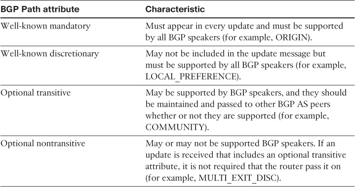
The following list highlights the typical BGP route selection (from the highest to the lowest preference):
1. Prefer highest weight (Cisco proprietary, local to router)
2. Prefer highest local preference (global within AS)
3. Prefer route originated by the local router
4. Prefer shortest AS path
5. Prefer lowest origin code (IGP < EGP < incomplete)
6. Prefer lowest MED (from other AS)
7. Prefer eBGP path over iBGP path
8. Prefer the path through the closest IGP neighbor
9. Prefer oldest route for eBGP paths
10. Prefer the path with the lowest neighbor BGP router ID
Note
For more information about BGP path selection, refer to the document “BGP Best Path Selection Algorithm,” at http://www.cisco.com/c/en/us/support/docs/ip/border-gateway-protocol-bgp/13753-25.html.
BGP as the Enterprise Core Routing Protocol
Most enterprises prefer IGPs such as OSPF as the core routing protocol to provide end-to-end enterprise IP reachability. However, in some scenarios, network designers may prefer a protocol that can provide more flexible and robust routing policies and can cover single and multirouted domains with the ability to facilitate a diversified administrative control approach.
For example, an enterprise may have a large core network that connects different regions or large department networks, each with its own administrative control. To achieve that, we need a protocol that can provide interconnects between all the places in the network (PINs) and at the same time enable each group or region to maintain the ability to control their network without introducing any added complexity when connecting the PINs. Obviously, a typical IGP implementation in the core cannot achieve that, and even if it is possible, it will be very complex to scale and manage.
In other words, when the IGP of large-scale global enterprises network reaches the borderline of its scalability limits within the routed network, which usually contains a high number of routing prefixes, and a high level of flexibility is required to support “splitting routed networks” into multiple failure domains with distributed network administration, BGP is the ideal candidate protocol as the enterprise core routing protocol.
BGP in the enterprise core can offer the following benefits to the overall routing architecture:
![]() A high degree of responsiveness to new business requirements, such as business expansion, business decline, innovation (IPv6 over IPv4 core), and security policies like end-to-end path separation (for example, MP-BGP + MPLS in the core)
A high degree of responsiveness to new business requirements, such as business expansion, business decline, innovation (IPv6 over IPv4 core), and security policies like end-to-end path separation (for example, MP-BGP + MPLS in the core)
![]() Design simplicity (separating complex functional areas, each into its own routed region within the enterprise)
Design simplicity (separating complex functional areas, each into its own routed region within the enterprise)
![]() Flexible domain control by supporting administrative control per routing domains (per region)
Flexible domain control by supporting administrative control per routing domains (per region)
![]() More flexible and manageable routing policies that support intra- and interdomain routing requirements
More flexible and manageable routing policies that support intra- and interdomain routing requirements
![]() Improved scalability because it can significantly reduce the number of prefixes that regional routing domains need to hold and process
Improved scalability because it can significantly reduce the number of prefixes that regional routing domains need to hold and process
![]() Optimized network stability by stressing fault isolation domain boundaries (for example, at IGP island edges), where any control plane instability in one IGP/BGP domain will not impact other routing domains (topology and reachability information hiding principle)
Optimized network stability by stressing fault isolation domain boundaries (for example, at IGP island edges), where any control plane instability in one IGP/BGP domain will not impact other routing domains (topology and reachability information hiding principle)
However, network designers need to consider some limitations or concerns that BGP might introduce to the enterprise routing architecture when used as the core routing protocol:
![]() Convergence time: In general, BGP convergence time during a change or following a failure event is slower than IGP. However, this can be mitigated to a good extent when advanced BGP fast convergence techniques are well tuned, such as BGP (PIC).
Convergence time: In general, BGP convergence time during a change or following a failure event is slower than IGP. However, this can be mitigated to a good extent when advanced BGP fast convergence techniques are well tuned, such as BGP (PIC).
![]() Staff knowledge and operational complexity: BGP in the enterprise core can simplify the routing design. However, additional knowledge and experience for the operation staff is required because the network will be more complex to troubleshoot, especially if multiple control policies in different directions are applied for control and traffic engineering purposes.
Staff knowledge and operational complexity: BGP in the enterprise core can simplify the routing design. However, additional knowledge and experience for the operation staff is required because the network will be more complex to troubleshoot, especially if multiple control policies in different directions are applied for control and traffic engineering purposes.
![]() Hardware and software constraints: Some legacy or low-end network devices either do not support BGP or may require a software upgrade to support it. In both cases, there is a cost and possibility of a maintenance outage for the upgrade. This might not always an acceptable or supported practice by the business.
Hardware and software constraints: Some legacy or low-end network devices either do not support BGP or may require a software upgrade to support it. In both cases, there is a cost and possibility of a maintenance outage for the upgrade. This might not always an acceptable or supported practice by the business.
Enterprise Core Routing Design Models with BGP
This section highlights and compares the primary and most common design models that network designers and architects can consider for large-scale enterprise networks with BGP as the core routing protocol (as illustrated in Figure 2-46 through Figure 2-49). These design models are based on the design principle of dividing the enterprise network into a two-tiered hierarchy. This hierarchy includes a transit core network to which a number of access or regional networks are attached. Typically, the transit core network runs BGP and glues the different geographic areas (network islands) of the enterprise regional networks. In addition, no direct link should interconnect the regional networks. Ideally, traffic from one regional network to another must traverse the BGP core. However, each network has unique and different requirements. Therefore, all the design models discussed in this section support the existence or addition of backdoor links between the different regions; remember to always consider the added complexity to the design with this approach:
![]() Design model 1: This design model has the following characteristics:
Design model 1: This design model has the following characteristics:
![]() iBGP is used across the core only.
iBGP is used across the core only.
![]() Regional networks use IGP only.
Regional networks use IGP only.
![]() Border routers between each regional network and the core run IGP and iBGP.
Border routers between each regional network and the core run IGP and iBGP.
![]() IGP in the core is mainly used to provide next-hop (NHP) reachability for iBGP speakers.
IGP in the core is mainly used to provide next-hop (NHP) reachability for iBGP speakers.
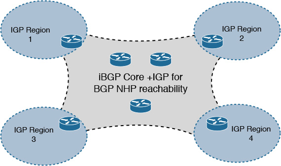
![]() Design model 2: This design model has the following characteristics:
Design model 2: This design model has the following characteristics:
![]() BGP is used across the core and regional networks.
BGP is used across the core and regional networks.
![]() In this design model, each regional network has its own BGP AS number (ASN) (no direct BGP session between the regional networks).
In this design model, each regional network has its own BGP AS number (ASN) (no direct BGP session between the regional networks).
![]() Reachability information is exchanged between each regional network and the core over eBGP (no direct BGP session between regional networks).
Reachability information is exchanged between each regional network and the core over eBGP (no direct BGP session between regional networks).
![]() IGP in the core as well as at the regional networks is mainly used to provide NHP reachability for iBGP speakers in each domain.
IGP in the core as well as at the regional networks is mainly used to provide NHP reachability for iBGP speakers in each domain.
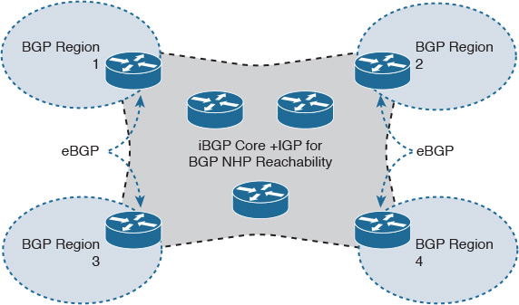
![]() Design model 3: This design model has the following characteristics:
Design model 3: This design model has the following characteristics:
![]() MP-BGP is used across the core (MPLS L3VPN design model).
MP-BGP is used across the core (MPLS L3VPN design model).
![]() MPLS is enabled across the core.
MPLS is enabled across the core.
![]() Regional networks can run either static IGP or BGP.
Regional networks can run either static IGP or BGP.
![]() IGP in the core is mainly used to provide NHP reachability for MP-BGP speakers.
IGP in the core is mainly used to provide NHP reachability for MP-BGP speakers.
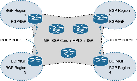
![]() Design model 4: This design model has the following characteristics:
Design model 4: This design model has the following characteristics:
![]() BGP is used across the regional networks.
BGP is used across the regional networks.
![]() In this design model, each regional network has its own BGP ASN.
In this design model, each regional network has its own BGP ASN.
![]() Reachability information is exchanged between the regional networks directly over direct eBGP sessions.
Reachability information is exchanged between the regional networks directly over direct eBGP sessions.
![]() IGP can be used at the regional networks to provide local reachability within each region and may be required to provide NHP reachability for BGP speakers in each domain (BGP AS).
IGP can be used at the regional networks to provide local reachability within each region and may be required to provide NHP reachability for BGP speakers in each domain (BGP AS).
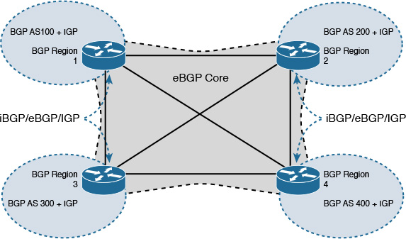
These designs are all valid and proven design models; however, each has its own strengths and weaknesses in certain areas, as summarized in Table 2-9. During the planning phase of network design or design optimization, network designers or architects must select the most suitable design model as driven by other design requirements, such as business and application requirements (which ideally must align with the current business needs and provide support for business directions such as business expansion).
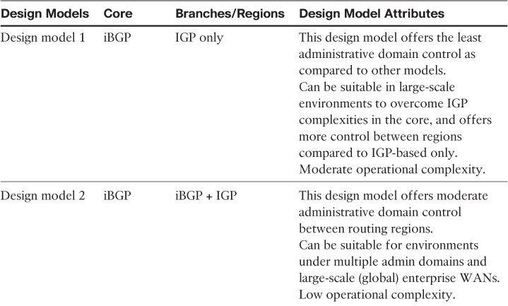
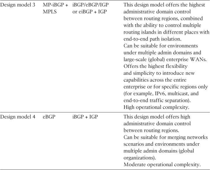
IGP or control plane complexity referred to in the table above is in comparison to the end to end IGP based design model, specifically across the core.
BGP Shortest Path over the Enterprise Core
BGP as a path-vector control plane protocol normally prefers the path with the smallest number of autonomous systems when traversing multiple autonomous systems when other attributes such as local_preference are the same (classical interdomain routing scenarios). Typically, in interdomain routing scenarios, the different routed domains have their own policies, which do not always need to be exposed to other routing domains. However, in the enterprise core with BGP scenarios, when a router selects a specific path based on the BGP AS-PATH attribute, the “edge eBGP” nodes cannot determine which path within the selected core or transit BGP core AS is the shortest (hypothetically, the optimal path). For instance, the scenario in Figure 2-50 depicts design model 2 of BGP enterprise core. The question is this: How can router A decide which path is the shortest (optimal) within the enterprise core (AS 65000)?
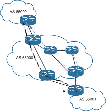
Accumulated IGP Cost for BGP (AIBGP) is an optional nontransitive BGP path attribute, designed to enhance shortest path selection in scenarios like the one in the example, where a large-scale network is part of a single enterprise with multiple administrative domains using multiple contiguous BGP networks (BGP core routing design model 2, discussed earlier in this section). Therefore, it is almost always more desirable that BGP consider the shortest path with the lowest metric across the transit BGP core. In fact, AIBGP replicates the behavior of link-state routing protocols in computing the distance associated with a path that has routes within a single flooding domain. Although the BGP MED attribute can carry IGP metric values, MED comes after several BGP attributes in the path selection process. In contrast, AIBGP is considered before the AS-PATH attribute when enabled in the BGP path selection process, which makes it more influential in this type of scenario:
1. Prefer highest weight (Cisco proprietary, local to router)
2. Prefer highest local preference (global within single AS)
3. Prefer route originated by the local router
5. Prefer shortest AS path
6. Prefer lowest origin code (IGP < EGP < incomplete)
7. Prefer lowest MED (from other AS)
8. Prefer eBGP path over iBGP path
9. Prefer the path through the closest IGP neighbor
It is obvious that AIBGP can be a powerful feature to optimize the BGP path selection process across a transit AS. However, network designers must be careful when enabling this feature because when AIBGP is enabled, any alteration to the IGP routing can lead to a direct impact on BGP routing (optimal path versus routing stability).
BGP Scalability Design Options and Considerations
This section discusses the primary design options to scale BGP in general at an enterprise network grade. Chapter 6, “Service Provider MPLS VPN Services Design,” extends these concepts and discusses the control plane and BGP scalability design considerations of service provider grade networks.
The natural behavior of BGP can be challenging when the size of the network grows to a large number of BGP peers, because it will introduce a high number of route advertisements, along with scalability and manageability complexities and limitations. According to the default behavior of BGP, any iBGP-learned route will not be advertised to any iBGP peer (the typical BGP loop-prevention mechanism, also known as the iBGP split-horizon rule). This means that a full mesh of iBGP peering sessions is required to maintain full reachability across the network. On this basis, if a network has 15 BGP routers within an AS, a full mesh of iBGP peering will require (15(15 – 1) / 2) = 105 of iBGP sessions to manage within an AS. Consequently, it will be a network that has a large amount of configuration associated with a high probability of configuration errors, and is complex to troubleshoot and has very limited scalability. However, BGP has two main proven techniques that you can use to reduce or eliminate these limitations and complexities of the BGP control plane:
![]() Route reflection (described in RFC 2796)
Route reflection (described in RFC 2796)
![]() Confederation (described in RFC 3065).
Confederation (described in RFC 3065).
BGP Route Reflection
Route reflection is a BGP route advertisement mechanism based on relaying the iBGP-learned routes from other iBGP peers. This process involves a special BGP peer or set of peers called route reflectors (RRs). These RRs can alter the classical iBGP spilt-horizon rule by re-advertising the BGP route that was received from iBGP peers to other iBGP peers, also known as route reflector clients, which can significantly reduce the total number of iBGP sessions, as illustrated in Figure 2-51. Moreover, RRs reflect routes to nonclient iBGP peers as well, in certain cases.
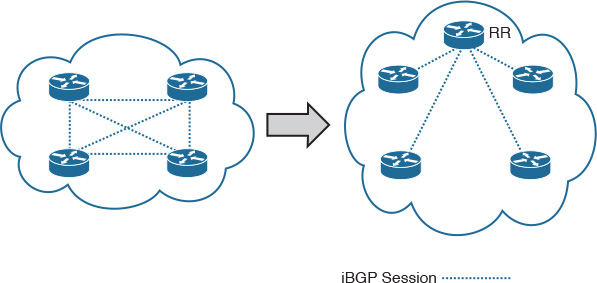
Figure 2-52 summarizes RR route advertisement rules based on three primary route sources and receivers in terms of the BGP session type (eBGP, iBGP- RR-client, and iBGP - non-RR-client).
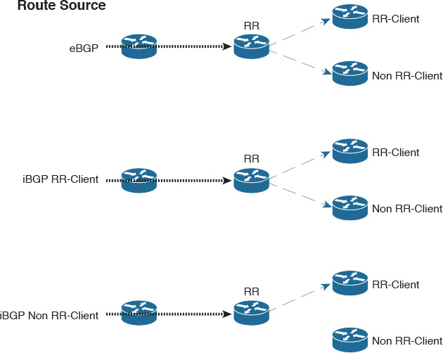
It is obvious from the figure that the route(s) sourced from an iBGP non-RR client peer(s) will not be re-advertised by the RR to another iBGP non-RR client peer(s) [24].
As a result, the concept of RR can help network designers avoid the complexities and limitations associated with iBGP full-mesh sessions, where more scalable and manageable designs can be produced. However, BGP RR can introduce new challenges that network designers should take into account, such as redundancy, optimal path selection, and network convergence. These points are covered in the subsequent sections, as well as in other chapters throughout this book.
Route Reflector Redundancy
In BGP environments, RRs can introduce a single point of failure to the design if no redundancy mechanism is considered. RR clustering is designed to provide redundancy, where typically two (or more) RRs can be grouped to serve one or more iBGP clients. With RR clustering, technically, BGP use a special 4-byte attributes called CLUSTER_ID. If any pair of RRs has the same CLUSTER_ID, this means that they are part of one RR cluster. Each route exchanged between those RRs in the same cluster will be ignored and not installed in their BGP routing table if this route identified by the receiving RR has the same CLUSTER_ID attribute that is being used. However, in some situations, it is recommended that two redundant RRs be configured with different CLUSTER_IDs for an increased level of BGP routing redundancy. For instance, the RR client in Figure 2-53 is multihomed to two RRs. If each RR is deployed with a different CLUSTER_ID, the RR client will continue to be able to reach prefix X, even after the link with RR 1 fails.
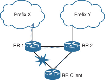
In contrast, if RR 1 and RR 2 were deployed with the same CLUSTER_ID, after this failure event the RR client in Figure 2-53 would not be able to reach Prefix X. This is because the CLUSTER_ID attribute mechanism will stop propagation of a route from RR 1 to RR 2 with the same CLUSTER_ID.
Furthermore, two BGP attributes were created specifically to optimize redundant RR behavior, especially with regard to avoiding routing information loops (for example, duplicate routing information). If the redundant RRs are being deployed in different clusters, the two attributes are ORIGINATOR_ID and CLUSTER_LIST.
RR Logical and Physical Topology Alignment
As discussed earlier in Chapter 1, the physical topology forms the foundation of many design scenarios, including BGP RRs. In fact, with BGP RRs, the logical and physical topologies must be given special consideration. They should be as congruent as possible to avoid any undesirable behaviors, such as suboptimal routing and routing loops. For example, the scenario depicted in Figure 2-54 is based on an enterprise network that uses BGP as the core routing protocol (based design model 1, discussed earlier in this chapter). In this scenario, the data center is located miles away from the campus core and is connected over two dark fiber links. The enterprise campus core routers C and D are configured as BGP RR (same RR cluster) to aggregate iBGP sessions of the campus buildings and data center routers. Data center aggregation router E is the iBGP client of core RR D, and the data center aggregation router F is the iBGP client of core RR C.
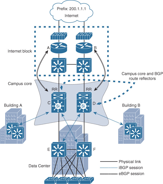
If the prefix 200.1.1.1 is advertised by both Internet edge routers (A and B), typically router A will advertise it to core router C, and router B will advertise it to core router D over eBGP sessions. Then, each RR will advertise this prefix to its clients. (RR C will advertise it to data center aggregation router F, and RR D will advertise to data center aggregation router E.) Up to this stage, there is no issue. However, when routers E and F try to reach prefix 200.1.1.1, a loop will be formed, as follows:
Note
For simplicity, this scenario assumes that both campus cores (RR) advertise the next-hop IPs of the Internet edge routers to all the campus blocks.
![]() Based on the design in Figure 2-54, data center aggregation E will have the next hop to prefix 200.1.1.1 as Internet edge router B.
Based on the design in Figure 2-54, data center aggregation E will have the next hop to prefix 200.1.1.1 as Internet edge router B.
![]() Data center aggregation F will have next hop to prefix 200.1.1.1 as Internet edge router A.
Data center aggregation F will have next hop to prefix 200.1.1.1 as Internet edge router A.
![]() Data center aggregation E will forward the packets destined to prefix 200.1.1.1 to data center aggregation F. (Based on physical connectivity and IGP, the Internet edge router B is reachable via data center aggregation F from the data center aggregation E point of view.)
Data center aggregation E will forward the packets destined to prefix 200.1.1.1 to data center aggregation F. (Based on physical connectivity and IGP, the Internet edge router B is reachable via data center aggregation F from the data center aggregation E point of view.)
![]() Because data center aggregation F has prefix 200.1.1.1, which is reachable through A, it will then send the packet back to data center aggregation E, as illustrated in Figure 2-55.
Because data center aggregation F has prefix 200.1.1.1, which is reachable through A, it will then send the packet back to data center aggregation E, as illustrated in Figure 2-55.
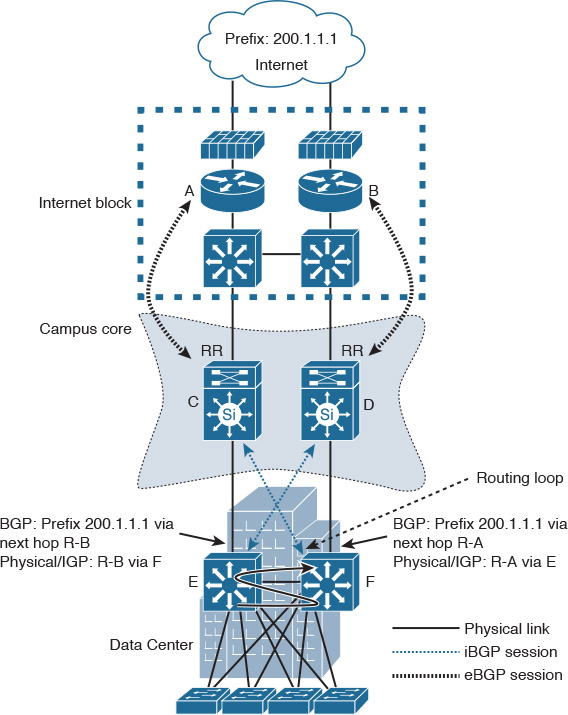
This loop was obviously formed because there is no alignment (congruence) between iBGP-RR topology and the physical topology. The following are three simple possible ways to overcome this design issue and to continue using RRs in this network:
![]() Add a physical link directly between E and D and between F and C, along with an iBGP session over each link to the respective core router. (It might take a long time to provision a fiber link, or it might be an expensive solution from the business point of view.)
Add a physical link directly between E and D and between F and C, along with an iBGP session over each link to the respective core router. (It might take a long time to provision a fiber link, or it might be an expensive solution from the business point of view.)
![]() Align the iBGP-RR peering with physical topology by making E the iBGP client to RR C and F the iBGP client to RR D (the simplest solution), as illustrated in Figure 2-56.
Align the iBGP-RR peering with physical topology by making E the iBGP client to RR C and F the iBGP client to RR D (the simplest solution), as illustrated in Figure 2-56.
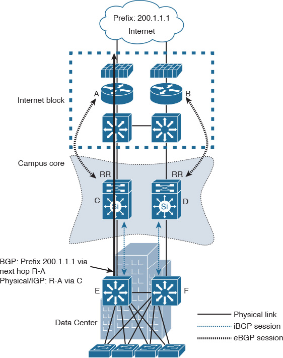
![]() Add a direct link between core RRs, place each RR in different RR cluster along with direct iBGP session between them. (This might add control plane complexity in this particular scenario to align IGP and BGP paths without alignment between the physical topology and iBGP client to RR sessions.)
Add a direct link between core RRs, place each RR in different RR cluster along with direct iBGP session between them. (This might add control plane complexity in this particular scenario to align IGP and BGP paths without alignment between the physical topology and iBGP client to RR sessions.)
One of the common limitations of the route reflection concept in large BGP environments is the possibility of suboptimal routing. This point is covered in more detail later in this book.
Update Grouping
Update grouping helps to optimize BGP processing overhead by providing a mechanism that groups BGP peers that have the same outbound policy in one update group, and updates are then generated once per group. By integrating this function with BGP route reflection, each RR update message can be generated once per update group and then replicated for all the RR clients that are part of the relevant group, as depicted in Figure 2-57 [25].
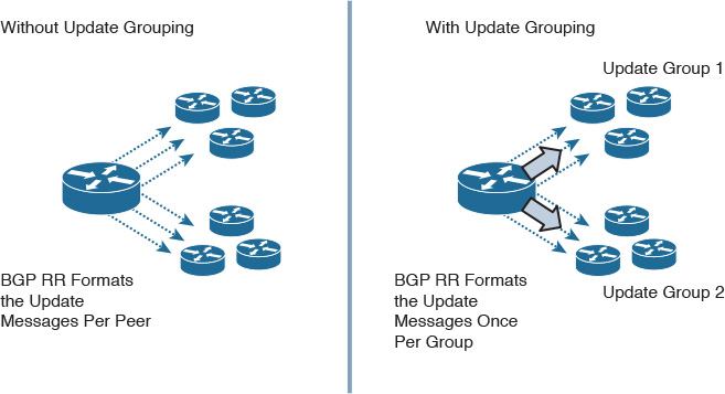
Technically, update grouping can be achieved by using peer group or peer template features, which can enhance BGP RR functionality and simplify the overall network operations in large BGP networks by
![]() Making the configuration easier, less error prone, and more readable
Making the configuration easier, less error prone, and more readable
![]() Lowering CPU utilization
Lowering CPU utilization
![]() Speeding up iBGP client provisioning (because they can be configured and added quickly)
Speeding up iBGP client provisioning (because they can be configured and added quickly)
BGP Confederation
The other option to solve iBGP scalability limitations in large-scale networks is through the use of confederations. The concept of a BGP confederation is based on splitting a large iBGP domain into multiple (smaller) BGP domains (also known as sub-autonomous systems). The BGP communication between these sub- autonomous systems is formed over eBGP session (a special type of eBGP session referred to as intra-confederation eBGP session) [24]. Consequently, the BGP network can scale and support a larger number of BGP peers because there is no need to maintain a full mesh among the sub-autonomous systems; however, within each sub-AS iBGP, full mesh is required, as illustrated in Figure 2-58.
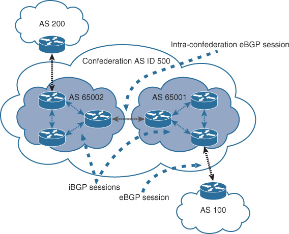
Note
The intra-confederation eBGP session has a mixture of both iBGP and eBGP characteristics. For example, NEXT_HOP, MED, and LOCAL_PREFRENCE attributes are kept between sub-autonomous systems. However, the AS_PATH is changed with updates across the sub-autonomous systems.
Note
The confederations appear as a single AS to external BGP autonomous systems. Because the sub-AS topology is invisible to external peering BGP autonomous systems, the sub-AS is also removed from the eBGP update sent to any external eBGP peer.
In large iBGP environments like a global enterprise (or Internet service provider [ISP] type of network), you can use both RR and confederation jointly to maximize the flexibility and scalability of the design. As illustrated in Figure 2-59, confederation can help to split the BGP AS into sub-autonomous systems, where each sub-AS can be managed and controlled by a different team or business unit. At the same time, within each AS, the RR concept is used to reduce iBGP full-mesh session complexity. In addition, network designers must make sure that IGP metrics within any given sub-AS are lower than those between sub-autonomous systems to avoid any possibility of suboptimal routing issues within the confederation AS.
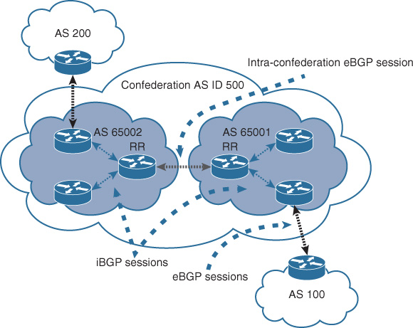
To avoid BGP route oscillation, which is associated with RRs or confederations in some scenarios, network designers must consider deploying higher IGP metrics between sub-autonomous systems or RR clusters than those within the sub-AS or cluster.
Note
Although BGP route reflection combined with confederation can maximize the overall BGP flexibility and scalability, it may add complexity to the design if the combination of both is not required. For instance, when merging two networks with a large number of iBGP peers in each domain, confederation with RR might be a feasible joint approach to optimize and migrate these two networks if it does not compromise any other requirements. However, with a large network with a large number of iBGP peers in one AS that cannot afford major outages and configuration changes within the network, it is more desirable to optimize using RR only rather than combined with confederation.
Confederation Versus Route Reflection
The most common dilemma is whether to use route reflection or confederation to optimize iBGP scalability. The typical solution to this dilemma, from a design point of view, is “it depends.” Like any other design decision, deciding what technology or feature to use to enhance BGP design and scalability depends on different factors. Table 2-10 highlights the different factors that can help you narrow down the design decision with regard to BGP confederation versus route reflection.
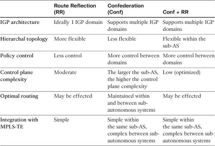
Again, there is no 100 percent definite answer. As a designer, you can decide which way to go based on the information and architecture you have and the goals that need to be achieved, taking the factors highlighted in Table 2-10 into consideration.
Further Reading
“BGP Case Studies”: http://www.cisco.com/c/en/us/support/docs/ip/border-gateway-protocol-bgp/26634-bgp-toc.html
“Load Sharing with BGP in Single and Multihomed Environments: Sample Configurations”: http://www.cisco.com
“Designing Scalable BGP Designs”: http://www.ciscopress.com/articles/article.asp?p=1763921&seqNum=7
BGP Route Reflection - An Alternative to Full Mesh IBGP, RFC 2796: http://www.ietf.org
BGP Route Reflection: An Alternative to Full Mesh Internal BGP (IBGP), RFC 4456: http://www.ietf.org
BGP MULTI_EXIT_DISC (MED) Considerations, RFC 4451: http://www.ietf.org
Route Redistribution Design Considerations
Route redistribution refers to the process of exchanging or injecting routing information (typically routing prefixes) between two different routing domains or protocols. However, route redistribution between routing domains does not always refer to the route redistribution between two different routing protocols. For example, redistribution between two OSPF routing domains where the border router runs two different OSPF instances (process) represents the redistribution between two routing domains using the same routing protocol. Route redistribution is one of the most advanced routing design mechanisms commonly relied on by network designers to achieve certain design requirements, such as the following:
![]() Merger and acquisition scenarios. Route redistribution can sometimes facilitate routing integration between different organizations.
Merger and acquisition scenarios. Route redistribution can sometimes facilitate routing integration between different organizations.
![]() In large-scale networks, such as global organizations, where BGP might be used across the WAN core and different IGP islands connect to the BGP core, full or selective route redistribution can facilitate route injection between these protocols and routing domains in some scenarios.
In large-scale networks, such as global organizations, where BGP might be used across the WAN core and different IGP islands connect to the BGP core, full or selective route redistribution can facilitate route injection between these protocols and routing domains in some scenarios.
![]() Route redistributions can also be used as an interim solution during the migration from one routing protocol to another.
Route redistributions can also be used as an interim solution during the migration from one routing protocol to another.
Note
None of the preceding points can be considered as an absolute use case for route redistribution, because the use of route redistribution has no fixed rule or standard design. Therefore, network designers need to rely on experience when evaluating whether route redistribution needs to be used to meet the desired goal or whether other routing design mechanisms can be used instead, such as static routes.
Route redistribution can sometimes be as simple as adding a one-line command. However, the impact of it sometimes leads to major network outages because of routing loops or the black-holing of traffic, which can be introduced to the network if the redistribution was not planned and designed properly. That is why network designers must have a good understanding of the characteristics of the participating routing protocols and the exact aim of route redistribution. In general, route redistribution can be classified into two primary models, based on the number of redistribution boundary points.
![]() Single redistribution boundary point
Single redistribution boundary point
![]() Multiple redistribution boundary points
Multiple redistribution boundary points
Single Redistribution Boundary Point
This design model is the simplest and most basic route redistribution design model; it has minimal complexities, if any. Typically, the edge router between the routing domains can perform either one- or two-way route redistribution based on the desired goal without any concern, as depicted in Figure 2-60. This is based on the assumption that there is no other redistribution point between the same routing domains anywhere else across the entire network.
However, if the redistributing border router belongs to three routing domains, the route that is sourced from another routing protocol cannot be redistributed into a third routing protocol on the same router. For instance, in Figure 2-61, the route redistributed from EIGRP into OSPF cannot be redistributed again from OSFP into RIP. (This behavior is described as a nontransitive attribute.)
Multiple Redistribution Boundary Points
Networks with two or more redistribution boundary points between routing domains require careful planning and design prior to applying the redistribution into the production network, because it can lead to a complete or partial network outage. The primary issues that can be introduced by this design are as follows:
![]() Routing loop
Routing loop
![]() Suboptimal routing
Suboptimal routing
![]() Slower network convergence time
Slower network convergence time
To optimize a network design that has two or more redistribution boundary points, network designers must consider the following aspects and how each may impact the network, along with the possible methods to address it based on the network architecture and the design requirements (for example optimal versus suboptimal routing):
![]() Metric transformation
Metric transformation
![]() Administrative distance
Administrative distance
Metric Transformation
Typically, each routing protocol has its own characteristic and algorithm to calculate network paths to determine the best path to use based on certain variables known as metrics. Because of the different metrics (measures) used by each protocol, the exchange of routing information between different routing protocols will lead to metric conversion so that the receiving routing protocol can understand this route, as well as be able to propagate this route throughout its routed domain. Therefore, specifying the metric at the redistribution point is important, so that the injected route can be understood and considered.
For instance, a common simple example is the redistribution from RIP into OSPF. RIP relies on hop counts to determine the best path, whereas OSPF considers link cost that is driven by the link bandwidth. Therefore, redistributing RIP into OSPF with a metric of 5 (five RIP hops) has no meaning to OSPF. Hence, OSPF assigns a default metric value to the redistributed external route. Furthermore, metric transformation can lead to routing loops if not planned and designed correctly when there are multiple redistribution points. For example, Figure 2-62 illustrates a scenario of mutual redistribution between RIP and OSPF over two border routers. Router A receives the RIP route from the RIP domain with a metric of 5, which means five hops. Router B will redistribute this route into the OSPF domain with the default redistribution metrics or any manually assigned metric. The issue in this scenario is that when the same route is redistributed back into the RIP domain with a lower metric (for example, 2), router A will see the same route with a better metric from the second border router. As a result, a routing loop will be formed based on this design (because of metric transformation).
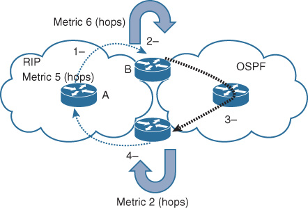
Hypothetically, this metric issue can be fixed by redistributing the same route back into the RIP domain with a higher metric value (for example, 7). However, this will not guarantee the prevention of routing loops because there is another influencing factor in this scenario, which is administrative distance (see the following section, “Administrative Distance,” for more detail). Therefore, by using route filtering or a combination of route filtering and tagging to prevent the route from being re-injected back into the same domain, network designers can avoid route looping issues in this type of scenario.
Administrative Distance
Some routing protocols assign a different administrative distance (AD) value to the redistributed route by default (typically higher than the locally learned route) to give it preference over the external (redistributed route). However, this value can be changed, which enables network designers and engineers to alter the default behavior with regard to route and path section. From the route redistribution design point of view, AD can be a concern that requires special design considerations, especially when there are multiple points of redistribution with mutual route redistribution.
To resolve this issue, either route filtering or route tagging jointly with route filtering can be used to avoid re-injecting the redistributed (external) route back into the same originating routing domain. You can tune AD value to control the preferred route. However, this solution does not always provide the optimal path when there are multiple redistribution border routers performing mutual redistribution. If for any reason AD tuning is used, the network designer must be careful when considering this option, to ensure that routing protocols prefer internally learned prefixes over external ones (to avoid unexpected loops or suboptimal routing behavior).
Route Filtering Versus Route Tagging with Filtering
Routing filtering and route tagging combined with route filtering are common and powerful routing policy mechanisms that you can use in many routing scenarios to control route propagation and advertisement and to prevent routing loops in situations where multiple redistribution boundary points are exits with mutual route redistribution between routing domains. However, these mechanisms have some differences that network designers must be aware of, as summarized in Table 2-11.
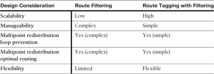
Based on the simple comparison in Table 2-11, it is obvious that route filtering is more suitable for small and simple filtering and loop-prevention tasks. In contrast, route filtering associated with route tagging can support large-scale and dynamic networks to achieve more scalable and flexible routing policies across routing domains.
For example, in the scenario illustrated in Figure 2-63, there are two boundary redistribution points with mutual redistribution between EIGRP and IS-IS in both directions deployed at R1 and 2. In addition, R10 is injecting external EIGRP route for an organization to communicate with their business partner; this route will typically have by default an AD value of 170.
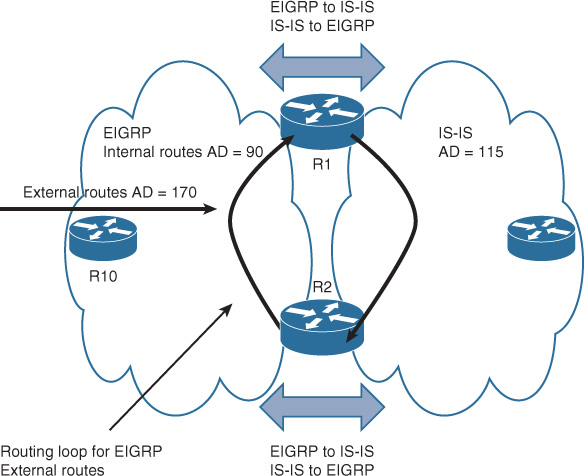
After this external route is injected into the EIGRP domain, internal users connected to the IS-IS domain started complaining that they could not reach any of the intended destinations located at their business partner network.
This design has the following technical concerns:
![]() Two redistribution boundary points
Two redistribution boundary points
![]() Mutual redistribution at each boundary point from a high AD domain (external EIGRP in this case) to a lower AD domain
Mutual redistribution at each boundary point from a high AD domain (external EIGRP in this case) to a lower AD domain
![]() Possibility of metric transformation (applicable to the external EIGRP route when redistributed back from IS-IS with better metrics)
Possibility of metric transformation (applicable to the external EIGRP route when redistributed back from IS-IS with better metrics)
As a result, a route looping will be formed with regard to the external EIGRP (between R1 and R2). With route filtering combined with tagging, as illustrated in Figure 2-64, both R1 and R2 can stop the re-injection of the redistributed external EIGRP route from IS-IS back into EIGRP again.
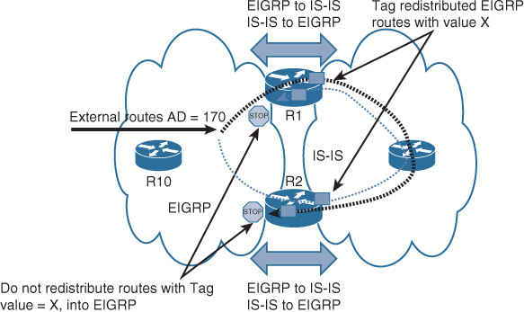
This is achieved by assigning a tag value to the EIGRP route when it is redistributed into IS-IS (at both R1 and R2). At the other redistribution boundary point (again R1 and R2) routes can be stopped from being redistributed into EIGRP again based on the assigned tag value. After you apply this filtering, the loop will be avoided, and path selection can be something like that depicted in Figure 2-65. With route tagging as in this example, network operators do not need to worry about managing and updating complicated access control lists (ACLs) to filter prefixes, because they can match the route tag at any node in the network and take action against it. Therefore, this offers simplified manageability and more flexible control.
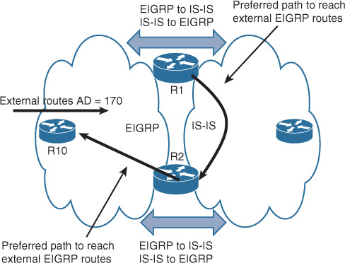
The optimal path, however, will not be guaranteed in this case unless another local filtering is applied to deny the EIGRP route from being installed in the local IS-IS routing table of the boundary routers. However, this must be performed only if optimal path is a priority requirement, to avoid impacting any potential loss of path redundancy. For instance, if R1. In Figure 2-65 filter the redistributed EIGRP external routes by “R2” from being installed into IS-IS local routing table (based on the assigned route tag by R2) optimal path can be achieved here. However if there is a LAN or hosts connected directly to R1, and R1 loses its connection to the EIGRP domain. In this case any device or network uses R1 as its gateway, will not be able to reach the EIGRP external routes (unless there is a default route, or a floating static route with higher AD, points to R2 within the IS-IS domain), in other words, to achieve optimal path, a second filtering layer is required at the ASBRs (R1 and R2 in this example) to filter the “redistributed” external EIGRP routes by the other IS-IS ASBR from being re-injected into IS-IS local routing table of the ASBR based on the route tag (refer to this sample example for more technical details,5). Also each ASBRs should use a default route (ideally static route, point to the other ASBR) to maintain redundancy to external prefixes in case of an ASBR link failure toward the EIGRP domain, as illustrated in Figure 2-66.
5. “Preventing route looping by using route tagging”, https://supportforums.cisco.com/document/32191/preventing-route-looping-using-route-tagging
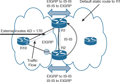
From design point of view, achieving optimal network design does not mean optimal path must always be considered. For example, as a network designer you must look at the bigger picture using the “holistic approach” highlighted previously in chapter 1, in order to evaluate and decide, what are the possible options to achieve the design requirements optimally?, and what can be the implications of each design option?. For instance in the scenario discussed above, if the IS-IS domain is receiving a default route from an internal node such as an Internet edge router. In this case, injecting a default route from the ASBRs (R1 and R2) most probably will break the Internet reachability for the IS-IS domain or any network directly connected to R1 and R2. Therefore, if both paths (over R1 and R2, with or without asymmetrical routing) technically satisfy the requirements for the communication between this organization and its partner network, in this case from network design perspective “optimal path” is not a requirement to achieve “optimal design”. Because, optimal path can introduce design and operational complexity as well as it may break the internet reachability in this particular scenario.
Note
Route tagging in some platforms require the IS-IS “wide metric” feature to be enabled in order for the route tagging to work properly, where migrating IS-IS routed domain from “narrow metrics to wide metrics” must be considered in this case6.
6. IETF RFC 3787, Recommendations for Interoperable IP Networks using Intermediate System to Intermediate System IS-IS
Note
If asymmetrical routing has a bad impact on the communications in the scenario above, between EIGRP and IS-IS domains, it can be avoided by tuning EIGRP metrics such as delay, when the IS-IS route redistributed into EIGRP to control path selection from EIGRP domain point of view and align it with the selected path from IS-IS side (to align both ingress and egress traffic flows).
Enterprise Routing Design Recommendations
This chapter discussed several concepts and approaches pertaining to Layer 3 control plane routing design. Table 2-12 summarizes the main Layer 3 routing design considerations and recommendations in a simplified way that you can use as a foundation to optimize the overall routing design.
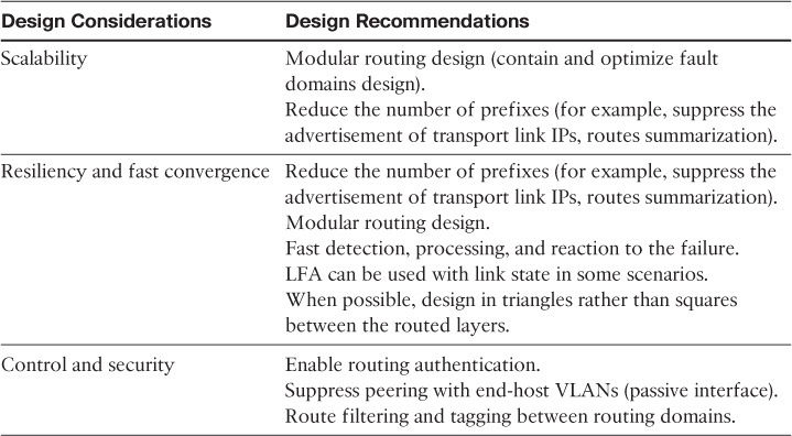
Determining Which Routing Protocol to Use
In large-scale enterprise networks with different modules and many remote sites, selecting a routing protocol can be a real challenge. Therefore, network designers need to consider the answers to the following questions as a foundation for routing protocol selection:
![]() What is the underlying topology, and which protocol can scale to a larger number of prefixes and peers?
What is the underlying topology, and which protocol can scale to a larger number of prefixes and peers?
![]() Which routing protocol can be more flexible, taking into account the topology and future plans (for example, integrating with other routing domains)?
Which routing protocol can be more flexible, taking into account the topology and future plans (for example, integrating with other routing domains)?
![]() Is fast convergence a requirement? If yes, which protocol can converge faster and at the same time offer stability enhancement mechanisms?
Is fast convergence a requirement? If yes, which protocol can converge faster and at the same time offer stability enhancement mechanisms?
![]() Which protocol can utilize fewer hardware resources?
Which protocol can utilize fewer hardware resources?
![]() Is the routing internal or external (different routing domains)?
Is the routing internal or external (different routing domains)?
![]() Which protocol can provide less operational complexity (for instance, easy to configure and troubleshoot)?
Which protocol can provide less operational complexity (for instance, easy to configure and troubleshoot)?
Although these questions are not the only ones, they cover the most important functional requirements that can be delivered by a routing protocol. Furthermore, there are some factors that you need to consider when selecting an IGP:
![]() Size of the network (for example, the number of L3 hops and expected future growth)
Size of the network (for example, the number of L3 hops and expected future growth)
![]() Security requirements and the supported authentication type
Security requirements and the supported authentication type
![]() IT staff knowledge and experience
IT staff knowledge and experience
![]() Protocol’s flexibility in modular network such as support of flexible route summarization techniques
Protocol’s flexibility in modular network such as support of flexible route summarization techniques
Generally speaking, EIGRP tends to be more simple and scalable in hub-and-spoke topology and over networks with three or more hierarchical layers, whereas link-state routing protocols can perform better over flat networks when flooding domains and other factors discussed earlier in this book are tuned properly. In contrast, BGP is the preferred protocol to communicate between different routing domains (external), as summarized in Figure 2-67.
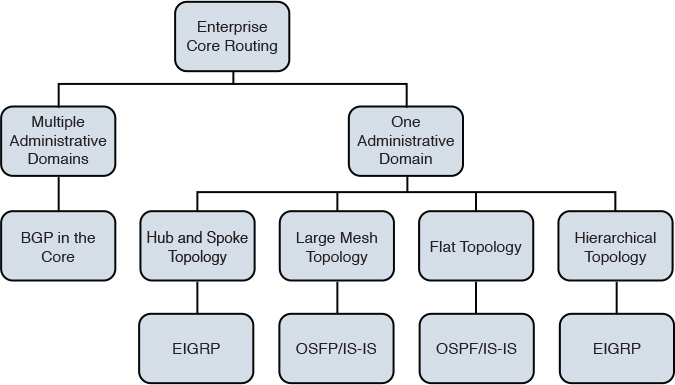
Moreover, the decision tree depicted in Figure 2-68 highlights the routing protocol selection decision to migrate from one routing protocol to another based on the topology used. This tree is based on the assumption that you have the choice to select the preferred protocol.
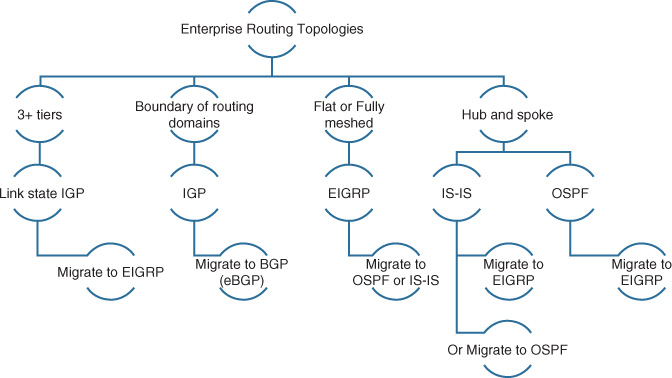
Summary
For network designers and architects to provide a valid and feasible network design (including both Layer 2 and Layer 3), they must understand the characteristics of the nominated or used control protocols and how each behaves over the targeted physical network topology. This understanding will enable them to align the chosen protocol behavior with the business, functional, and application requirements, to achieve a successful business-driven network design. Also, considering any Layer 2 or Layer 3 design optimization technique such as route summarization may introduce new design concerns (during normal or failure scenarios) such as suboptimal routing. Therefore, the impact of any design optimization must be taken into consideration and analyzed, to ensure the selected optimization technique will not induce new issues or complexities to the network that could impact its primary business functions. Ideally the requirements of the business critical-applications and business priorities should drive design decisions.