
Chapter 9. Network High-Availability Design
Business application and service availability considerations in today’s modern converged networks have become a vital design element, especially now that many businesses understand the IT network’s availability impact and cost to the organization, whether it is an enterprise or service provider network. Practically, the cost of a service downtime due to a network outage can take different forms: tangible, intangible, or a combination of both. Some of the common losses that can be caused by network downtime (which normally impact the business either directly or indirectly) are as follows:
![]() Tangible such as data loss, revenue loss, and reduced user productivity
Tangible such as data loss, revenue loss, and reduced user productivity
![]() Intangible such as degraded reputation, customer dissatisfaction, and employees dissatisfaction
Intangible such as degraded reputation, customer dissatisfaction, and employees dissatisfaction
Consequently, the availability of the different IT infrastructure and services becomes one of the common primary requirements of today’s modern businesses that rely to a large extent on technology services to facilities achieving their business goals, such as mobility, cloud-hosted services, e-government services, Internet of Things (IoT), and smart connected cities. Therefore, many of these businesses with converged next-generation networks are aiming to achieve the five nines of network and IT services availability when developing their network designs.
Note
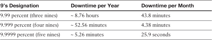
The term five nines usually refers to the degree of service availability. Literally, it refers to 99.999 percent of the functional time of a system, which can be translated to time of downtime per month/year as listed in Table 9-1.
Although it is hard to achieve the absolute five nines, it is becoming common nowadays for it to be targeted as an availability requirement in network service level agreements (SLAs). Achieving a true end-to-end five nines level of availability for a given service or application is not an easy goal to achieve because there are multiple influencing factors. For example, multiple factors impact the overall level of availability of any given application in a data center, such as network infrastructure availability, server component availability, storage availability, and all other components that are part of this application architecture on higher layers such as database, front-end application, and so on. Therefore, this chapter focuses only on the network infrastructure part and the design aspects and considerations that pertain to the network elements only (elements that helps to optimize the overall availability of the other elements carried over the network such as critical business applications).
Note
As discussed earlier in this book, the need for network availability is increasing with the increased adoption of converged types of network and service consolidation. However, several variables dictate the level of network availability. It is not always the case that every part of the network requires the same level of network availability. In other words, the high level of availability is not always a common requirement.
Although network availability is not always a common requirement, it must be evaluated based on different criteria such as level of criticality and business priorities, which can specify the level of impact of the downtime on the business. In addition, sometimes it is too difficult to define when the network is down. For instance, is network downtime based on a specific application’s downtime, or is it based on specific part of the network, such as the data center? In fact, business requirements, goals, and the level of impact caused by the downtime with regard to these business priorities and goals can determine the standards of how network downtime is defined.
In general, the term network availability is an operations parameter reflected by the ratio of the time a network can be considered functional and performing as expected. Moreover, a system is seen as reliable when functioning without failure over a certain period of time. In fact, a system’s reliability can be measured either by the level of its operational quality within a given time slot (when the system was up and running) until the system went to a down state, which is also known as mean time between failures (MTBF = Total operational time / Number of failures), or by calculating a system’s failure rate (Number of failures / Total operational time).
The term operational quality here refers to some scenarios where a system might be technically up, yet is not performing its functions at the minimum required level. This means that the system not delivering the intended service or performing a function reliably even if is technically up. It is important to note that system reliability is one of the primary contributing elements to achieving the ultimate level of system or network availability.
The importance of system reliability is illustrated in the following case, where there is a network designed with a high level of availability (including redundant components). However, the interconnections between the core components of this network have low reliability. Examples of low reliability include the following:
![]() Unreliable line cards used at the core node.
Unreliable line cards used at the core node.
![]() The transport medium is unreliable, and the links keep flapping.
The transport medium is unreliable, and the links keep flapping.
Despite the fact that this network was designed with high-availability considerations, the low level of reliability of the core components in this network will impact the overall service availability.
However, the mean time to repair (MTTR) reflects the actual time required to repair a system from a failure condition. The following standard formula shows the correlation between availability, MTBF, and MTTR to calculate a system’s availability:
Availability = MTBF / (MTBF + MTTR)
Based on this formula, it is obvious that increasing the MTBF and decreasing MTTR can offer an improved overall level of availability. Thus, you can improve the availability of a network by optimizing the capability of its elements, such as the interconnecting transport links, to function without failures. A reliable network must be designed to tolerate at least a single component failure. Some designs may require the network to cater for multiple failures to meet certain design requirements. This usually translates into more redundant components, higher cost, and probably higher operational complexity.
Hypothetically, the more redundant paths we add to the network design, the higher the MTBF we can achieve. However, increasing MTBF is only half of the job. Therefore, network designers must consider how to reduce the repair time as well. Technically, adding more redundancy, which means increasing the parallelism here (redundant paths/links) leads to a higher MTTR at the network control plane layer. This will result in an increased control plane complexity and probably slower convergence time. In sum, for network designers to achieve the desired level of network availability, there must either be very highly reliable components end to end that reduce the probability of failure to a minimum or there must be redundant components that can take over in the event of a failure (reducing the possibility of failures versus reducing complete network outages).
Many recent industry studies and reports show that the majority of system downtime occurs because of either a deficiency in design analysis, testing (proof of concept [POC]), or operational mistakes. The minority of system downtime results from hardware or software failures. Therefore, decreasing the possibility of service or network outages can be more efficient and achievable than focusing only on eliminating any system or network component failure possibility. Consequently, this chapter always focuses on how to balance between having a reliable and fault-tolerant design to achieve the intended goal in a resilient and effective manner.
Fault Tolerance
In general, network fault tolerance can be defined as the capability of a network to continue its service (no downtime) in the event of any component failure, with minimal service interruption using a redundant component that can take over in transparent fashion. Ideally, this should be unnoticeable by the end users or applications. However, the operating quality may decrease, depending on the considerations for the post-failure situation, with regard to whether the redundant component can fully handle the load or partially handle it.
In addition, some businesses deem it acceptable for their networks to stay operational with degraded quality, rather than facing a complete network failure. In other words, a network can be considered fault tolerant when it offers the capability to function (fully or partially) for the duration of any network component failure, usually over a redundant component. Commonly, the more network nodes and components that are added, the more likely it is for network high availability to be undermined. Therefore, network designers need to consider how to optimize these types of designs and reduce single points of failure to achieve the desired level of the network uptime. To achieve the desired level of network availability and a high level of resiliency to cater for different types of failure conditions, the following fault-tolerance design aspects must be considered:
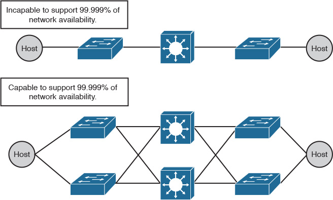
![]() Network level redundancy: It is also referred to as network path redundancy, and is essential to catering to link failures, such as fiber cuts, incorrect cabling, and so on. It is uncommon in LAN environments that end hosts connect with dual links at the access layer. Even though this will reduce the end-to-end reliability level, it is almost always acceptable as long as path redundancy is from the access layer onward (excluding data center high-availability [HA] considerations, because redundant connections are critical at the server access layer), as illustrated in Figure 9-1.
Network level redundancy: It is also referred to as network path redundancy, and is essential to catering to link failures, such as fiber cuts, incorrect cabling, and so on. It is uncommon in LAN environments that end hosts connect with dual links at the access layer. Even though this will reduce the end-to-end reliability level, it is almost always acceptable as long as path redundancy is from the access layer onward (excluding data center high-availability [HA] considerations, because redundant connections are critical at the server access layer), as illustrated in Figure 9-1.
![]() Device and component redundancy: Typically, redundant nodes provide redundancy during a node failure triggered by hardware or software. There are two types of node-level redundancies: redundant nodes and redundant components within a single device. You can use one or both types, based on the level of availability required and the targeted network environment (criticality). Considerations regarding passing traffic through the failure (for example, using redundant supervisors) versus passing traffic around the failure (using redundant devices) are primary influencing factors to the choice here as well. In addition, remember that redundant components (for example, redundant line cards for the uplinks) help to increase the overall level of system reliability. In general, redundant devices with diverse network paths offer better resiliency compared to a single device with redundant components. That said, a device with redundant components is more feasible for nodes that represent a single point of failure, such as a provider edge (PE) node in service provider networks.
Device and component redundancy: Typically, redundant nodes provide redundancy during a node failure triggered by hardware or software. There are two types of node-level redundancies: redundant nodes and redundant components within a single device. You can use one or both types, based on the level of availability required and the targeted network environment (criticality). Considerations regarding passing traffic through the failure (for example, using redundant supervisors) versus passing traffic around the failure (using redundant devices) are primary influencing factors to the choice here as well. In addition, remember that redundant components (for example, redundant line cards for the uplinks) help to increase the overall level of system reliability. In general, redundant devices with diverse network paths offer better resiliency compared to a single device with redundant components. That said, a device with redundant components is more feasible for nodes that represent a single point of failure, such as a provider edge (PE) node in service provider networks.
![]() Operational redundancy: Although the focus is almost always on how to optimize network redundancy and availability during unplanned failure scenarios, it is also important to consider how to provide redundancy during planned network outages, such as using in-service software upgrade (ISSU) or software maintenance update (SMU) capabilities.
Operational redundancy: Although the focus is almost always on how to optimize network redundancy and availability during unplanned failure scenarios, it is also important to consider how to provide redundancy during planned network outages, such as using in-service software upgrade (ISSU) or software maintenance update (SMU) capabilities.
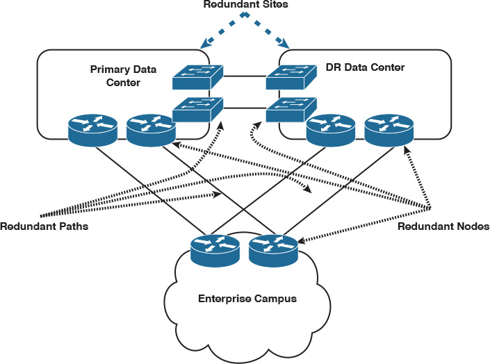
![]() Network architecture: The network architecture itself can facilitate, to a large degree, achieving an optimized level of availability. For instance, a hierarchical network design stresses redundancy at multiple layers to overcome any possible single point of failure. The other good example is “how” Clos architecture (TRILL or VxLAN based) helps to achieve large scale-out expansion in data center networks with several redundant components at the spines level without introducing complexity to the overall architecture. Furthermore, design redundancy at site or module level can help achieve optimized business and service availability for critical sites. A typical example of this is a disaster recovery (DR) data center with data center interconnect (DCI), as illustrated in Figure 9-2.
Network architecture: The network architecture itself can facilitate, to a large degree, achieving an optimized level of availability. For instance, a hierarchical network design stresses redundancy at multiple layers to overcome any possible single point of failure. The other good example is “how” Clos architecture (TRILL or VxLAN based) helps to achieve large scale-out expansion in data center networks with several redundant components at the spines level without introducing complexity to the overall architecture. Furthermore, design redundancy at site or module level can help achieve optimized business and service availability for critical sites. A typical example of this is a disaster recovery (DR) data center with data center interconnect (DCI), as illustrated in Figure 9-2.
Note
In Figure 9-2, the network can operate in an active-standby or active-active manner using the available redundant paths/components.
Note
In any network, fault tolerance relies on different process and mechanisms to achieve the desired level of switchover to the backup component, as discussed in subsequent sections.
Fate Sharing and Fault Domains
It is important that network architects and designers understand the difference and relation between fate sharing and fault domains. Fate sharing refers to the philosophy of system design in which a single system is constructed of multiple subsystems or components, with a failure of one subcomponent leading to a complete system failure (sharing the same fate). For instance, a failure of the CPU of a smartphone will normally lead to a complete device failure as a result of a single subcomponent failure. Moreover, in the networking world, fate sharing also refers to the scenarios where multiple virtual networks share a single network infrastructure (more specifically, single network element such as a physical link with multiple subinterfaces where each subinterface carries a different virtual network).
However, fault domain, as highlighted earlier in this book, refers to a domain where multiple systems reside under a single domain (physical or logical) and a failure in one component can impact all other components within the same domain, such as flooding of updates or error messages. Let’s consider the following example to demonstrate the impact and relationship between these concepts.
The scenario illustrated in Figure 9-3 shows two data center networks interconnected over a Layer 2 DCI. In addition, some virtualized networks are interconnected over the same DCI over a generic routing encapsulation (GRE) tunnel (with Multiprotocol Label Switching [MPLS] Layer 3 virtual private networking [L3VPN] enabled over the GRE tunnel). In this scenario, if any failure happens to the MPLS labels inside this tunnel, all the virtual networks passing through this tunnel will be impacted (sharing the same fate) as a result of a subcomponent failure of the entire MPLS L3VPN over GRE solution.
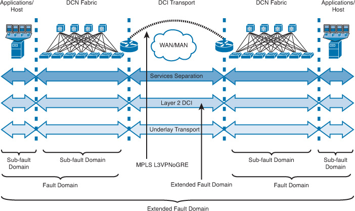
Similarly, the failure of the DCI in this particular scenario will lead to the failure of the multiple virtual networks carried over the GRE tunnel and of the extended VLAN over the Layer 2 DCI, resulting in a fate sharing situation as well. Another common terminology applicable here is the shared risk link group (SRLG), which is commonly used in traffic engineering designs where multiple links share a single point of failure, in which all the links pass through one network node (for example, all the cables are going into a single device on the same line card). A failure of this node or any subcomponent (such as the line card where the links terminate) will usually lead to complete failure for all the networks that have their links passing through this node (the SRLG point).
Moreover, as shown in Figure 9-3, each Layer 2 segment in each data center (DC) represents a fault domain. Extending the LAN over the DCI, however, will in turn lead to extending the fault domain of each DC to the other one. For instance, any host MAC flooding in an extended VLAN in one DC will be propagated across the DCI to the other DC. Layer 2 flooding may lead to DCI congestion, which will usually impact all other traffic passing over this path, including the GRE tunnel. For instance, if a host or node fails in one of the DCs, in some situations this may lead to a significant amount of flooding within a single failure domain (in this scenario, the failure domain extended across the DCI), which most probably will lead to congestion of the DCI link. As a result, all the virtual networks passing over the MPLS L3VPN over GRE will be impacted as well. In other words, the impact of a failure in a fault domain can affect all the systems in that domain, unlike fate sharing, which is normally limited to a given system or subcomponent of the entire network such as the GRE tunnel (described in the example), or it can be a group of MPLS Traffic Engineering (MPLS-TE) tunnels passing through an SRLG point.
One of the common design principles used to generate a design that is reliable and resilient enough and that caters for different failure scenarios (like the one described in this section) is called design for failure. This principle is discussed in the following section.
Network Resiliency Design Considerations
Today’s converged networks that carry voice and other real-time applications must recover in the event of network component failure in a few seconds (and sometimes within milliseconds) to effectively transmit traffic without affecting the end-user experience. Convergence times of less than one second could be highly desirable or a requirement for some networks, such as MPLS VPN service providers that offer virtual leased line (VLL) services. Therefore, network designers who aim to achieve the desired level of HA of network services must eliminate any single point of failure throughout the network. The network must recover during a component failure, such as link or node failure, to a redundant component that can continue the service operation. In other words, a redundant component that takes over in the event of a node or link failure must offer a fast network recovery (self-healing), also known as fast convergence, to maintain the desired level of network and service availability.
Furthermore, the redundant component should ideally take over within an acceptable period (for example, before mission-critical business application sessions restart) and handle the required functions reliably during the failure event. For example, you may have link- and device-level redundancy in your network that eliminates any single point of failure along the network path. However, in the event of any component failure, the network could take up to five minutes to recover from a simple failure to start using the redundant component. This may not be an acceptable resiliency level by the business, and this downtime in a next-generation converged network will impact many other services, such as mission-critical business applications and IP telephony services. Therefore, in this case, the availability goal from the business point of view is not optimally achieved, and so this does not justify the cost of buying and deploying redundant components.
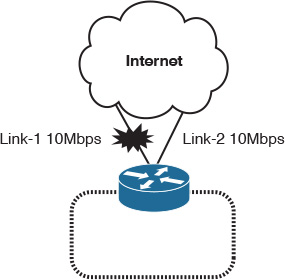
The other factor that needs to be considered is how reliably the redundant component can function following a network failure event to provide a truly resilient network design. For example, one common scenario where the increased parallelism (redundancy) may not lead to optimized service availability is with an enterprise Internet edge designed with multiple paths (links) with the intention to maximize the overall performance and provide a reliable solution.
However, the concern in this type of design is when the business requires maximizing the utilization of the available Internet links to increase the return on investment (ROI) of these links and to improve application and Internet service performance, as illustrated in Figure 9-4. If one of the Internet links goes down, the second link, with a maximum of 10 Mbps of bandwidth, will start handling 20 Mbps during the link 1 failure, which will lead to an almost 50 percent degraded performance (assuming both links are fully utilized). Therefore, unplanned redundancy probably leads to an undesirable outcome following a failure event.
For this enterprise to resolve this issue, it should add a third link to offload some of the traffic during any link failure. However, this solution will increase control plane and operational complexity and will add additional cost from the business point of view (capital expenditure [capex]). Alternatively, this enterprise needs to consider accurate link capacity planning, where each link utilization should not reach more than ~45 percent in a normal situation to cater to both links’ bandwidth requirements during a link failure scenario. Although this solution will incur additional cost, it adds no operational and control plane complexity to the existing design.
Note
Both solutions are valid, and the goal of this scenario is to highlight the importance of the planning and the analysis of the different failure scenarios and its impact on achieving a true resilient network design.
Network designers must aim to create a network design that offers resistance to failures (reliable) and that can recover quickly and reliably in the event of a failure (resilient). In this regard, network designers should always consider the analytical principle used today by public cloud providers such as Amazon AWS Cloud, commonly known as design for failure, in which network designers ensure that the possible failure scenarios (including root causes and the failure scenario’s impact on the business) have been analyzed and addressed within the design. Applying this design for failure principle facilitates the desired level of availability. It also helps network architects and designers identify and understand the impact and risk of different failure events on the business, such as the estimated outage period and to what degree this failure can disrupt business operations.
Consequently, when you design a network for failure with the objective of offering a highly fault-tolerant, reliable, and resilient network design, consider the following as you construct the foundation of the design architecture:
![]() Perform analysis of different downtime failure scenarios and their impact on the business’s critical functions and data to be aligned with the business’s expectations, such as recovery time objective (RTO) and recovery point objective (RPO) levels.
Perform analysis of different downtime failure scenarios and their impact on the business’s critical functions and data to be aligned with the business’s expectations, such as recovery time objective (RTO) and recovery point objective (RPO) levels.
![]() Optimize network services availability on higher layers to the desired level that meets business and user expectations, such as web-application firewalls, Domain Name System (DNS), and load balancers.
Optimize network services availability on higher layers to the desired level that meets business and user expectations, such as web-application firewalls, Domain Name System (DNS), and load balancers.
![]() Every network component should be redundant (when possible) to eliminate any single point of failure across the network path.
Every network component should be redundant (when possible) to eliminate any single point of failure across the network path.
![]() The network should be adequately capable of recovering in the event of a node or link failure with minimal or no service interruption during the recovery process, and without any operator intervention (resilient).
The network should be adequately capable of recovering in the event of a node or link failure with minimal or no service interruption during the recovery process, and without any operator intervention (resilient).
![]() The redundant component can continue to function at the desired level during a failure scenario (reliable resiliency).
The redundant component can continue to function at the desired level during a failure scenario (reliable resiliency).
![]() Classify and set recovery priorities from both business and technical points of view. (Critical functions and prerequisite services for other functions must always recover first.)
Classify and set recovery priorities from both business and technical points of view. (Critical functions and prerequisite services for other functions must always recover first.)
Note
The desired level of a network’s availability or convergence time will vary from business to business. Therefore, for the purpose of the CCDE exam, only consider fast network recovery time if it is explicitly required or implied through other requirements.
When designing a highly available and resilient network that can converge fast enough without impacting any business-critical activities or applications, network designers need to consider a number of things. In other words, it is not limited to the scope of tuning control plane timers; in fact, it is an end-to-end process. Network designers need to consider all the network layers involved in this convergence process to achieve a true and effective convergence.
As a network designer, start by asking the following questions to understand whether the network is performing at the desired level, and to meet application requirements and business expectations:
![]() The characteristics of business-critical applications: How much time does each business-critical application or service running on the network require before it loses its state or session? For instance, the CEO’s voice call might be dropped because of minor packet loss (over 3 percent of packet loss) during network convergence time.
The characteristics of business-critical applications: How much time does each business-critical application or service running on the network require before it loses its state or session? For instance, the CEO’s voice call might be dropped because of minor packet loss (over 3 percent of packet loss) during network convergence time.
![]() Network reaction: How long does the network take to converge following a component failure? You should consider end-to-end recovery time because the network might reconverge in some parts quicker than other parts and introduce microloops.
Network reaction: How long does the network take to converge following a component failure? You should consider end-to-end recovery time because the network might reconverge in some parts quicker than other parts and introduce microloops.
![]() Network security components: Are there network security devices in the path, such as firewalls? If yes, are they redundant? How quick is its failover process? Is it a stateful or stateless failover?
Network security components: Are there network security devices in the path, such as firewalls? If yes, are they redundant? How quick is its failover process? Is it a stateful or stateless failover?
Note
It is important to note that the target here is not only routing convergence, but the overall network convergence. As a network designer, always ask the question, “What can be done apart from the typical control plane timers to minimize loss in the event of a failure?”
This section discusses various mechanisms that network designers can consider to optimize network availability and convergence time to achieve the optimal targeted level of resiliency at different levels:
![]() Device-level resiliency
Device-level resiliency
![]() Protocol-level resiliency
Protocol-level resiliency
Note
As mentioned earlier, this chapter focuses only on network availability. In reality, the overall service and application availability must be measured end to end (at all layers; instance, if a voice control system [such as Cisco CallManager] is running on a cluster distributed across two data centers). In the event of the primary (active) data center failure, the network may reconverge in a few seconds, whereas Session Initiation Protocol (SIP)-based IP phones may take up to three minutes to register with the new active call control system because of a DNS failover delay (timeout duration).
Device-Level Resiliency
Device-level resiliency (also referred to as component resiliency) aims to maintain or keep traffic forwarding intact during a component failure at the network node level, such as routing processor failure. Therefore, it is critical for network designers to not get this concept confused with protocol-level resiliency, which usually aims to route traffic around the failed component. If routing protocols are tuned to converge quickly (subseconds), this will demolish the value of deploying device-level redundancy. Therefore, a balance between the device-level resiliency and the protocol-level must be considered when the device-level resiliency is a requirement.
Different protocols and mechanisms aim to offer a network design that can continue to forward traffic through a network node with a failure (such as a primary routing processor failure), with the assumption that a redundant routing processor is available on the same device. The following are the primary mechanisms used to achieve device-level resiliency:
![]() Stateful switchover (SSO): Allows the standby route processor to take immediate control and maintain connectivity protocols
Stateful switchover (SSO): Allows the standby route processor to take immediate control and maintain connectivity protocols
![]() Nonstop forwarding (NSF): Continues to forward packets until route convergence is complete
Nonstop forwarding (NSF): Continues to forward packets until route convergence is complete
![]() Graceful restart (GR): Reestablishes the routing information bases without churning the network
Graceful restart (GR): Reestablishes the routing information bases without churning the network
![]() Nonstop Routing (NSR): Continues to forward packets and maintains routing state
Nonstop Routing (NSR): Continues to forward packets and maintains routing state
GR and NSR suppress routing changes on peers to SSO-enabled devices during processor switchover events (SSO), reducing network instability and downtime. In addition, the following protocol-specific considerations must be taken into account with regard to device-level resiliency design:
![]() NSR is desirable in cases where the routing protocol peer does not support the RFCs necessary to support GR. However, it comes at a cost of using more system resources than would be used if the same session used GR.
NSR is desirable in cases where the routing protocol peer does not support the RFCs necessary to support GR. However, it comes at a cost of using more system resources than would be used if the same session used GR.
![]() For MPLS-enabled networks, you can use the following features to enhance network resiliency during a component failure:
For MPLS-enabled networks, you can use the following features to enhance network resiliency during a component failure:
![]() Label Distribution Protocol (LDP) GR (RFC 3478)
Label Distribution Protocol (LDP) GR (RFC 3478)
![]() LDP-IGP synchronization (RFC 5443)
LDP-IGP synchronization (RFC 5443)
![]() LDP session protection (based on the LDP targeted hello functionality defined in RFC 5036)
LDP session protection (based on the LDP targeted hello functionality defined in RFC 5036)
![]() Because NSR is a self-contained solution, it is more feasible for when the peer routing node is not under the same administrative authority, as is the case with PE-CE (customer edge) routers. In addition, NSR improves the overall system’s reliability.
Because NSR is a self-contained solution, it is more feasible for when the peer routing node is not under the same administrative authority, as is the case with PE-CE (customer edge) routers. In addition, NSR improves the overall system’s reliability.
Network edge nodes such as PE devices in a service provider (SP) environment represent a single point of failure; therefore, features such as NSF and SSO, along with redundant components (redundant supervisors), are more common with these devices to provide redundant intra-chassis route processors and network resilience. Backbone network nodes, however, are more commonly deployed with protocol-level resiliency, in which network convergence depends on protocol convergence to an alternate primary path such as using tuned interior gateway protocol (IGP) for fast convergence or MPLS-TE fast reroute (FRR).
Operationally, a major consequence and benefit of SSO is that adjacent devices do not see a link failure when the route processor switches from the primary to the hot standby route processor. This applies to route processor switchovers only. If the entire chassis were to lose power or fail, or a line card failure were to occur, the links would fail, and the peer would detect such an event. Of course, this assumes point-to-point Gigabit Ethernet interfaces, Packet over SONET (POS) interfaces, and so on, where link failure is detectable. Even with NSF enabled, physical link failures are still detectable by a peer and override NSF awareness.1
1. http://www.cisco.com/en/US/technologies/tk869/tk769/technologies_white_paper0900aecd801dc5e2.html
Protocol-Level Resiliency
As highlighted earlier in this chapter, a resilient network is a network that can recover following any network failure event. Network recovery, however, refers to the overall required time for all network nodes participating in path calculation, and traffic routing and forwarding, to complete restructuring or updating network reachability information following a network component failure (for example, a link or node failure). This is usually performed at the control plane “protocol” level. The faster the convergence time, the quicker a network can react to any change in the topology. There are two primary network recovery approaches:
![]() Network restoration approach: A reactive approach that computes an alternate primary path to reroute traffic over it after detection of a network component failure. Normal Open Shortest Path First (OSPF) behavior after failure of the primary path is a good example of this approach.
Network restoration approach: A reactive approach that computes an alternate primary path to reroute traffic over it after detection of a network component failure. Normal Open Shortest Path First (OSPF) behavior after failure of the primary path is a good example of this approach.
![]() Network protection approach: This approach is a proactive concept that precomputes (or signals) a backup loop-free alternate path in advance before any failure event. In the event any failure is detected, the protected traffic is moved over to the backup path transparently (commonly within 100 ms or less).
Network protection approach: This approach is a proactive concept that precomputes (or signals) a backup loop-free alternate path in advance before any failure event. In the event any failure is detected, the protected traffic is moved over to the backup path transparently (commonly within 100 ms or less).
In general, at any given layer in the network, network protection approach offers faster convergence than restoration. However, in some scenarios, it can be an expensive option, such as with optical layer protection. It may also introduce an added layer of complexity to the design, control plane, and the manageability of the network, such as using a full mesh of MPLS-TE tunnels among a large number of nodes.
That said, there is no single best approach; it always depends on the business goals and functional and application requirements to be satisfied. For instance, a five-minute recovery time might not be an issue for a retail business, whereas in a financial services environment, this duration may cost the business hundreds of thousands of dollars. Therefore, the cost of a failure here can justify the expensive but fast and reliable network recovery solution. The subsequent sections cover the two primary approaches of protocol-level resiliency in more detail.
Network Restoration
As described earlier, the concept of network restoration or convergence refers to the time required for network nodes to recompute their routing and forwarding tables and calculate a new primary path reactively following a network component failure. Convergence time is an essential measurement of “how long” routers within a routing domain can take to reach the state of convergence. In addition, network and protocol convergence can be seen as a primary performance indicator. However, achieving the desired level of convergence time is not as simple as tuning a few protocol timers. In fact, multiple elements determine how quickly and reliably a network or routing protocol convergence can occur at different network layers. Hence, any design that aims to optimize a routing protocol convergence time has to take all of these elements into consideration. These elements are categorized as follows:
![]() Event detection
Event detection
![]() Event propagation
Event propagation
![]() Event processing
Event processing
![]() Update routing and forwarding tables
Update routing and forwarding tables
As depicted in Figure 9-5, each of these elements contributes to the overall convergence time. Therefore, the optimization of these elements collectively reduces the time a network needs to recover following a failure event.
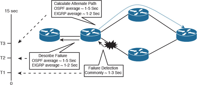
To achieve the desired convergence time, all these elements must be considered. In other words, the optimization of one or a subset of these elements only does not necessarily lead to an optimized convergence time at the desired level. The following subsections, considering the different characteristic of each routing protocol, discuss how each of these elements influence the overall convergence time.
Event Detection Considerations
The declaration or detection of a peer failure is a primary element in optimizing network convergence, simply because it is the trigger to starting the network recovery process. The detection of a failure in networking can happen at different layers, such as the physical layer (IP over dense wavelength-division multiplexing [IPoDWDM]), data link layer (Point-to-Point Protocol / High-level Data Link Control [PPP/HDLC] keepalive messages), network layer (routing protocols), and up to the application layer. This section focuses on the network convergence at the network layer and below.
The most commonly used mechanism to detect a link failure and to check a control plane neighbor’s reachability is a “poll-driven” mechanism that relies on the Layer 3 control plane hello messages and hold timers, also commonly referred to as fast hellos. Due to the deployment simplicity of fast hellos, it is one of the most common mechanisms used in many networks today. However, in large-scale networks and networks with strict convergence time requirements, this mechanism introduces several limitations that may inhibit achieving the desired level of network convergence, such as the following:
![]() Scalability limitations: Typically occur in a network with a large number of Layer 3 control plane peers
Scalability limitations: Typically occur in a network with a large number of Layer 3 control plane peers
![]() Hardware resource consumption overhead: Normally, when the number of Layer 3 control plane peers increases, there will be potential CPU spikes that may introduce what are called false positives, where links might be incorrectly declared to be broken
Hardware resource consumption overhead: Normally, when the number of Layer 3 control plane peers increases, there will be potential CPU spikes that may introduce what are called false positives, where links might be incorrectly declared to be broken
To overcome the limitations of this poll-based failure detection mechanism, you can use an event-driven mechanism instead to add more reliable and faster detection capabilities with low overhead. The most common and proven protocol used for this purpose is the bidirectional forwarding detection (BFD). BFD operates independently of the Layer 3 control plane protocols based on the concept of hello or heartbeat type protocols. Moreover, BFD supports several control protocols such as Hot Standby Routing Protocol (HSRP), link-state, Border Gateway Protocol (BGP), and Enhanced Interior Gateway Routing Protocol (EIGRP), where each protocol can register with BFD to be notified when BFD detects a neighbor loss. As a result, these routing protocols can overcome the delay and limitations of the poll-based failure detection mechanism that is mainly based on protocol hello and hold timers. BFD offers a more simplified, reliable, and faster failure detection mechanism (within tens of milliseconds).
Note
Typically, routers connected over direct point-to-point links can be notified by the physical layer when a link fails, which accelerates failure detection by the Layer 3 nodes. BFD, however, enables network operators to achieve fast failure detection in scenarios where two or more Layer 3 nodes are interconnected over a Layer 2 switched network. In this scenario, these Layer 3 nodes do not need to rely on control plane fast hellos and hold timers to detect a Layer 3 peer link or node failure.
Besides the BFD-supported control protocols highlighted earlier, BFD is also supported with static routing, and based on the status of the associated BFD session, the static route is either added to or withdrawn from the Routing Information Base (RIB) table, which makes static routing more reliable.
In BGP environments, however, the IGP fast failure detection and subsecond convergence time may lead to temporary traffic black-holing because of the typical significant convergence time difference between IGP and BGP by default. For instance, in a typical enterprise network with BGP in the core or an MPLS VPN SP network, such as a Carrier Ethernet (MPLS L2VPN Ethernet VPN [EVPN] based), the operator may deploy its backbone IGP to detect a link’s failure and recover within one second to achieve fast-converging next-generation L2VPN transport. As a result, in this scenario after a link or node failure, IGP will converge in one second, whereas Multiprotocol BGP (MP-BGP) continues to use the same next hop to reach a MAC addresses advertised in BGP by a remote PE for a given EVPN-EVI (EPVN instance) that is no longer a valid next hop after the last failure event. This is because MP-BGP, in this situation, is still relying on the poll mechanism to deal with the changes in the RIB, where “every 60 seconds, the BGP scanner recalculates best path for all prefixes.” In other words, MP-BGP in this case may take up to 60 seconds to realize that the next hop is not anymore useable, and during this 60 second time period between scan cycles, IGP instability, invalid BGP next-hop, or other network failures can cause black holes and routing loops to temporarily form2.
2. “BGP Support for Next-Hop Address Tracking”, http://www.cisco.com
However, with BGP next-hop tracking (NHT) and the address tracking filter (ATF), if the next-hop IP of MGP-BGP routes changes because of link failure followed by fast failure detection and IGP convergence, BGP now can respond faster (by lowering the response time to next-hop changes for prefixes installed in the RIB) without the need to wait for the initial 60 seconds of the “scanner.” Therefore, it is always important to understand what other protocols are running over the network besides IGP, and to understand how fast failure detection and IGP fast convergence (for example, subsecond convergence time) will impact the performance and behavior of these protocols or applications.
In spite of the benefits of deploying fast failure detection (subsecond), the following are the main design concerns that must be considered when designing a fast convergence network with subsecond failure detection:
![]() Instability: In many situations, very fast failure detection can lead to flapping and can add high overhead on the network hardware and routing protocols because of unnecessary processing and calculation.
Instability: In many situations, very fast failure detection can lead to flapping and can add high overhead on the network hardware and routing protocols because of unnecessary processing and calculation.
![]() Break device-level resiliency: Very fast failure detection breaks the concept of device-level resiliency described earlier (SSO, NSF, NSR). Therefore, the design cannot mix these two approaches (passing traffic through the failure versus passing traffic around the failure). This is because it may take about one to two seconds for the secondary route processor (supervisor) to start the failover process. Therefore, detecting a failure too fast (such as using BFD or too-low-tuned fast hellos) will usually override the entire failover process.
Break device-level resiliency: Very fast failure detection breaks the concept of device-level resiliency described earlier (SSO, NSF, NSR). Therefore, the design cannot mix these two approaches (passing traffic through the failure versus passing traffic around the failure). This is because it may take about one to two seconds for the secondary route processor (supervisor) to start the failover process. Therefore, detecting a failure too fast (such as using BFD or too-low-tuned fast hellos) will usually override the entire failover process.
![]() Traffic black-holing: If the fast failure detection was not aligned properly with the other protocols and overlay technologies running over IGP, such as MP-BGP or IP tunneling keepalives, the network could possibly face temporary traffic black-holing after a failure.
Traffic black-holing: If the fast failure detection was not aligned properly with the other protocols and overlay technologies running over IGP, such as MP-BGP or IP tunneling keepalives, the network could possibly face temporary traffic black-holing after a failure.
Event Propagation and Processing Considerations
The propagation of a network failure event and the computation process after detecting the failure refers to the reaction of the control plane to describe the failure event to other peers and finding an alternate primary path, respectively. With regard to route convergence design considerations, what is important is how long each of these processes takes and how they can be optimized. In general, there are two primary influencing factors to optimize these processes:
![]() Protocol characteristic and its timers: This varies based on the control plane protocol in use.
Protocol characteristic and its timers: This varies based on the control plane protocol in use.
![]() Network design: This is common for all protocols, to a large extent.
Network design: This is common for all protocols, to a large extent.
As discussed earlier, each protocol has different characteristics and its own philosophy for propagating and processing routing changes and updates, whether its link state, distance vector, or path vector. Typically, when a failure is detected by a Layer 3 node running a link-state routing protocol, this node and any other node connected to the failed component will start propagating this event by flooding OSPF link-state advertisements (LSAs) or Intermediate System-to-Intermediate System link-state packets (IS-IS LSPs) to every node within the link-state flooding domain. The overall event propagation duration of each LSA/LSP is normally governed by three primary timers: generation delay, reception delay, and processing delay.
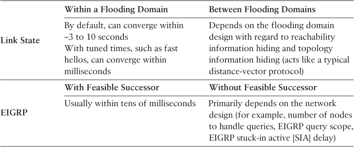
Both IS-IS and OSPF, however, can use the incremental shortest path first SPF (iSPF) algorithm to optimize SPF computations and converge faster in response to network events and topology changes, simply because iSFP is more efficient than the full SPF algorithm. In contrast, EIGRP uses a completely different logic and sequence. EIGRP finds an alternate path (usually precalculated using EIGRP feasible successor, thus avoiding the entire EIGRP query process, which significantly improves EIGRP convergence following failure event detection). Then, EIGRP propagates the failure to the peers. Table 9-2 highlights the fundamental differences between link state and EIGRP with regard to each protocol’s convergence characteristic.
In contrast, with BGP as a path-vector protocol, its propagation philosophy of a failure event is based on the propagation of withdrawal update messages that normally can be tuned to reduce the overall duration. In addition, the tuning of the following elements that technically influence BGP transport offer an optimized BGP performance to handle a large number of prefixes during the propagation and processing following a failure in the BGP path:
![]() TCP maximum segment size (MSS)
TCP maximum segment size (MSS)
![]() TCP window size
TCP window size
![]() Path maximum transmission unit (MTU) discovery (RFC 1191)
Path maximum transmission unit (MTU) discovery (RFC 1191)
![]() BGP minimum route advertisement interval (MRAI)
BGP minimum route advertisement interval (MRAI)
![]() Router queues (for example, input queue hold)
Router queues (for example, input queue hold)
Note
BGP prefix-independent convergence (PIC), described later in this chapter, helps to significantly enhance BGP convergence time.
From a network design perspective, the following common design considerations can help to optimize the convergence time and improve network stability:
![]() Fault isolation: As discussed earlier, fault isolation has a significant influence on enhancing the operation of routing protocols and reducing the amount of information that needs to be propagated. It also enhances the scope of the topology information shared between logical routing domains, which ultimately reduces hardware overhead utilization and the time required for the Layer 3 nodes to complete the propagation, processing, and finding an alternate primary path.
Fault isolation: As discussed earlier, fault isolation has a significant influence on enhancing the operation of routing protocols and reducing the amount of information that needs to be propagated. It also enhances the scope of the topology information shared between logical routing domains, which ultimately reduces hardware overhead utilization and the time required for the Layer 3 nodes to complete the propagation, processing, and finding an alternate primary path.
![]() Number of routes: One of the primary influencers on the overall time required for propagating, processing, and updating routing and forwarding tables is the number of the effected prefixes with a network change. Therefore, the information reachability hiding techniques discussed earlier in this book will help considerably in optimizing network convergence time and at the same time reduce the impact on its stability. For instance, with EIGRP, in addition to route summarization, stub routers help to reduce the processing of the DUAL algorithm and the scope of query messages. This will enhance the overall EIGRP convergence time while keeping the network as stable as possible (minimal to zero impact on the remote stub networks). Similarly, with link-state protocols, such as IS-IS (L1) or OSPF, in stub areas or totally stubby areas, the router’s LSA database size can be reduced, which will enhance the overall convergence time as well.
Number of routes: One of the primary influencers on the overall time required for propagating, processing, and updating routing and forwarding tables is the number of the effected prefixes with a network change. Therefore, the information reachability hiding techniques discussed earlier in this book will help considerably in optimizing network convergence time and at the same time reduce the impact on its stability. For instance, with EIGRP, in addition to route summarization, stub routers help to reduce the processing of the DUAL algorithm and the scope of query messages. This will enhance the overall EIGRP convergence time while keeping the network as stable as possible (minimal to zero impact on the remote stub networks). Similarly, with link-state protocols, such as IS-IS (L1) or OSPF, in stub areas or totally stubby areas, the router’s LSA database size can be reduced, which will enhance the overall convergence time as well.
![]() Multiple available paths: The availability of a second path can significantly enhance convergence time. Therefore, with EIGRP, it is essential that the design supports the precomputation of EIGRP feasible successor. In addition, apart from EIGRP feasible successor, if a BGP speaker has two available paths to a given destination network, the time required to process and find an alternate path can be eliminated because there is already an alternate path. However, unlike IGP, achieving this with BGP is sometimes challenging, especially in large networks where there is an route reflector (RR) in the path. The features and techniques covered in Chapter 5, “Service Provider Network Architecture Design,” are designed specifically to overcome these limitations in some BGP topologies. Similarly, availability of a second route in link state will offer an almost immediate failover with minimal to zero service interruption.
Multiple available paths: The availability of a second path can significantly enhance convergence time. Therefore, with EIGRP, it is essential that the design supports the precomputation of EIGRP feasible successor. In addition, apart from EIGRP feasible successor, if a BGP speaker has two available paths to a given destination network, the time required to process and find an alternate path can be eliminated because there is already an alternate path. However, unlike IGP, achieving this with BGP is sometimes challenging, especially in large networks where there is an route reflector (RR) in the path. The features and techniques covered in Chapter 5, “Service Provider Network Architecture Design,” are designed specifically to overcome these limitations in some BGP topologies. Similarly, availability of a second route in link state will offer an almost immediate failover with minimal to zero service interruption.
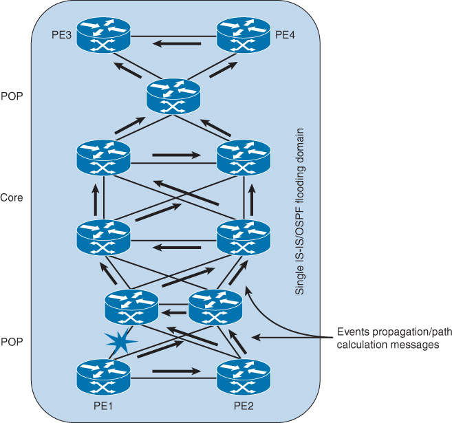
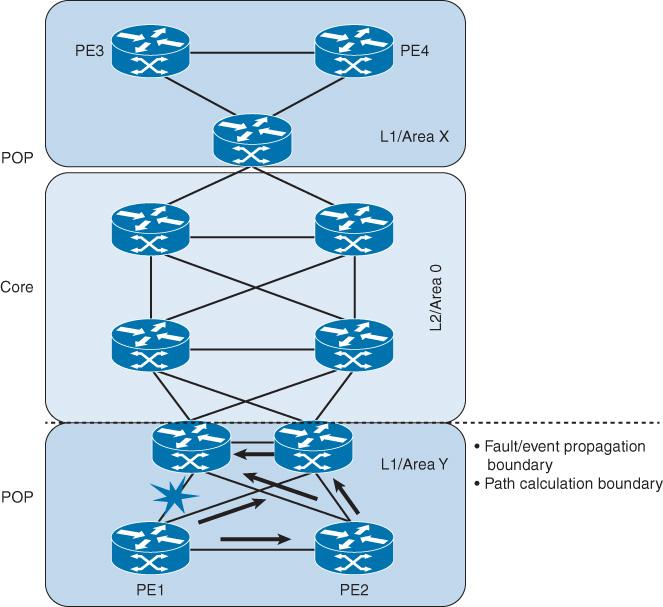
Let’s consider the scenario illustrated in Figure 9-6 to demonstrate the impact of link-state design on convergence time and the overall network stability following a network failure event. In this scenario, if PE1 needs to calculate the possible paths to reach PE3 loopback IP, there is a high number of possible paths to be considered part of the path computation process. It is obvious that this design has an increased MTTR because of the high degree of parallelism (redundant paths). Therefore, when network designers evaluate a design like the one depicted in Figure 9-6, they should consider the following fundamental questions when there is a link or node failure:
![]() How many possible paths must PE1 calculate and process?
How many possible paths must PE1 calculate and process?
![]() How many routers will be notified about a single link failure?
How many routers will be notified about a single link failure?
![]() How many routers will not be effected by this failure, but yet will unnecessarily receive and process the update messages?
How many routers will not be effected by this failure, but yet will unnecessarily receive and process the update messages?
Note
Even if EIGRP were used in this design, the question is, “How big should the EIGRP query scope be?”
In conclusion, the design presented in this scenario will slow down the convergence time, stability, and the performance of the network, as well, because of the flat routing design, especially if there is a large number of prefixes carried by the control plane.
If you introduce the principle of fault isolation with IGP logical flooding domains (using IS-IS levels, OSPF areas, or EIGRP summarization) depending on the used control plane protocol, PE1 will have a significantly optimized topology because it will have a fewer number of paths to calculate to reach PE3 (the calculation and updates flooding will usually be up to the border of the flooding domain), as illustrated in Figure 9-7. As a result, the design offers faster network convergence time with a higher level of stability (fault isolation).
Note
It is important, from a design point of view, to understand the location and role of the node that needs to be optimized for network convergence (for instance, if it is a core router or edge [PE] router) because the impact of applying some optimizations techniques can differ. Typically, PE devices handle more customer routes; consequently, tuning IGP timers aggressively down may introduce noticeable stability and performance issues.
Updating the RIB and FIB
Updating the Routing Information Base (RIB) and Forwarding Information Base (FIB) are other influencing factors within the network convergence process. Typically, after the control plane updates the Layer 3 node RIB table, the updates are propagated and reflected to the FIB table (either centrally or distributed depending on the hardware platform architecture). Normally, any process containing prefix installation will first be impacted by the number of prefixes to be installed (the larger the number of prefixes, the longer the duration of installation). Therefore, for networks with a significantly large number of prefixes (thousands or hundreds of thousands of prefixes), this process will be impacted at both levels:
![]() Updating the RIB table
Updating the RIB table
![]() Populating the updates to the FIB table or tables
Populating the updates to the FIB table or tables
One common mechanism to optimize the prefix installation process is prefix prioritization, in which network operators can assign a higher priority for certain prefixes, such as loopback IPs, to establish an LDP session quickly (in MPLS networks) before other prefixes, such as BGP prefixes. Similarly, the BGP event-based VPN import helps to accelerate route installation, where (PE) nodes in an MPLS L3VPN environment can propagate VPN routes to the CE nodes without relying on the scan time delay. Furthermore, Link-state offers the flexibility to network operators to avoid packets loss (instability) when a network node reloads or recovers from a failure. In this particular scenario, IGP most probably will converge (build its routing table) before BGP, and some routers may start forward traffic through the just reloaded node, which may lead to packs’ loss. Because at this point of time, BGP is still rebuilding its routing tables (not fully populated with all IP prefixes). Link-state overcomes this issue by advertising routes with higher metrics “for a fixed period of time” after a node reload or a recovery from a failure. This ultimately will help to avoid impacting transit traffic that is currently using other alternate routes and gives BGP more time to rebuild its routing table. Technically to achieve this, OSPF uses the “wait-for-bgp” feature to send route-LSAs with infinity metric after a reload until BGP is converged or the predefined timer is expired, in the same way, IS-IS uses “set-overload-bit” to wait until BGP converged or the predefined timer is expired3.
3. “Uses of the Overload Bit with IS-IS”, “Using OSPF Stub Router Advertisement Feature”, http://www.cisco.com
Network Fast Restoration Versus Network Stability
Today’s converged networks carry sensitive real-time traffic (such as Voice over IP [VoIP] and business video) and should offer a relatively fast restoration time following any network failure event (usually by tuning routing protocol timers aggressively low). However, the very fast reaction may sensitize the network, causing it to potentially take an action and converge and reconverge again because of the very fast failure detection and protocol reaction for any simple link flap or packet loss. As a result, this will impact the overall stability of the network and probably will outweigh any benefit of the fast convergence.
Therefore, network designers must compromise between both (fast convergence and stability) to achieve a stable fast converging design. There are multiple ways at different layers to optimize the overall network stability when the network is tuned to converge quickly. For instance, a dampening mechanism can relatively mitigate the effect of network instability. Dampening mechanisms are applicable at the protocol and link level, such as link-state exponential backoff and IP interface dampening, respectively. In addition, link-state protocol “throttling” of SPF and LSA/LSP generation mitigates the impact of network instability, such as link flapping, to some extent.
Furthermore, the design considerations discussed earlier in this chapter and previous chapters in this book, such as fault isolation, can play a primary role in optimizing the overall network stability. This is because the flooding and bad behavior caused by an unstable component in one domain will be contained and will not be propagated across the entire network (multiple flooding domains concept). As a general rule of thumb, tuning control plane timers aggressively low should be done with very careful planning, considering the different design aspects and influencing factors, along with a thorough testing of multiple failure scenarios.
Microloops
Microloops, also known as transient loops, occur when different nodes in the network calculate new alternate paths following a failure event independently of each other and at different times. This behavior is typical in a ring full- or partial-meshed topology running the link-state control plane. For instance, in Figure 9-8, if host A is communicating with host B and the link between R3 and R5 fails, R5 will reconverge and send the traffic to R4. Assuming R4 is converged as well, it will usually then forward the traffic toward R1. If R1 has not converged yet, traffic will loop between these two nodes (R4 and R1). If the duration of this microloop is small, where the network can converge quickly, packets will usually loop for a short duration before their time to live (TTL) expires. Eventually, the packets from host A will reach host B in this scenario. However, if the application is very sensitive, such as voice traffic, this might lead to a call dropped or low voice quality. In other words, application characteristics and their level of tolerance must be considered here as well.
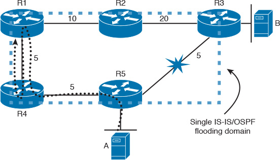
In contrast, if the duration of the microloop is long, in this scenario it may be because of the slow R1 convergence time. In this case, a packet’s TTL will normally expire, or the packet’s rate may exceed the available bandwidth. In both cases, it will result in packet drop. Practically, this type of microloop is not always an issue and is acceptable by many businesses. However, it might not be an acceptable behavior for other businesses. In these cases, where this type of microloop is unacceptable, network designers need to either use a triangle topology or a different approach to control network convergence in fully meshed, partially meshed, square, or ring topologies following a network component failure. This limitation can be resolved with the network protection approach, which is covered in the following section.
Note
R1 prefers the path via R4-R5 to reach R3 before the failure event in the scenario described earlier, because of the lower path cost.
Note
Network designers may use the microloop prevention feature described in IETF draft “litkowski-rtgwg-uloop-delay-xx” to mitigate the impact of link-state routing protocol transient loops during topology changes when possible.
Network Protection Approach
Although the network restoration approach is the most commonly used approach to optimize network recovery duration, this approach has the following limitations, which may impact the requirements of some networks:
![]() With the restoration approach, large-scale networks may face microloops (as discussed earlier) for a few seconds until the entire core and network has converged properly, which will usually lead to some packet loss within this duration.
With the restoration approach, large-scale networks may face microloops (as discussed earlier) for a few seconds until the entire core and network has converged properly, which will usually lead to some packet loss within this duration.
![]() Tuning routing protocol timers to react and converge very quickly is required to achieve subsecond network convergence time. However, this will result in reduced network stability, which increases the likelihood that the network may react to any simple packet loss. It will also add operational complexity in large networks with a large number of nodes.
Tuning routing protocol timers to react and converge very quickly is required to achieve subsecond network convergence time. However, this will result in reduced network stability, which increases the likelihood that the network may react to any simple packet loss. It will also add operational complexity in large networks with a large number of nodes.
In contrast, the network protection approach may be more suitable for satisfying the requirements of large-scale networks that need very fast convergence time (subsecond) without sacrificing network stability. Typically, with the network protection approach, the alternate path is always preestablished and does not need to wait for a protocol calculation across several devices throughout the network following network component failure detection. However, regardless of how fast the switchover method is, if the failure detection mechanism is slow it will overweigh the benefits of the FRR. Therefore, the issues and mechanisms discussed earlier in this chapter regarding failure detection must be considered to achieve a true fast convergence.
This section discusses the primary and most common technologies used to achieve the network protection approach. Each of these technologies can be deployed solely or in combination with other protocols, based on the goal to be achieved, supported features, targeted topology, and network environment.
MPLS-TE Fast Reroute
MPLS-TE fast reroute (MPLS-TE FRR) is commonly used by service provider networks and large-scale enterprise networks where fast recovery after failure detection is a fundamental requirement. It is normally driven by application requirements, such as real-time applications (VoIP), where a network has to reconverge following a network component failure in a relatively undetectable time from the application perspective. However, designing an MPLS-TE with FRR can be a complex task, especially when the network is large and has a large number of paths and nodes. Therefore, to select the right design approach, you must identify the goal to be achieved There are two primary MPLS-TE FRR approaches:
![]() Path protection (end to end): With MPLS-TE FRR, there are usually two LSPs used. The first one is the primary, and the second one is the presignaled backup LSP. The end-to-end FRR approach has some limitations with this behavior that network designers must consider [115]:
Path protection (end to end): With MPLS-TE FRR, there are usually two LSPs used. The first one is the primary, and the second one is the presignaled backup LSP. The end-to-end FRR approach has some limitations with this behavior that network designers must consider [115]:
![]() Resource overutilization: When the secondary path is preestablished, it will lead to what is known as double booking for the network resources, in particular bandwidth booking, with Resource Reservation Protocol (RSVP) to maintain the same bandwidth constraints as the primary LSP (TE tunnel) to keep the same level of the offered service level agreement (SLA) (1:1 protection).
Resource overutilization: When the secondary path is preestablished, it will lead to what is known as double booking for the network resources, in particular bandwidth booking, with Resource Reservation Protocol (RSVP) to maintain the same bandwidth constraints as the primary LSP (TE tunnel) to keep the same level of the offered service level agreement (SLA) (1:1 protection).
![]() Overprotection: This can occur when other mechanisms are used to protect a given set of links within the path, because this approach cannot protect links selectively along the path.
Overprotection: This can occur when other mechanisms are used to protect a given set of links within the path, because this approach cannot protect links selectively along the path.
![]() Longer restoration time: The path protection approach is usually based on a headend-controlled switchover; therefore, this behavior may lead to unexpected delays because it relies on the propagation time of RSVP error message to the headend node to perform the switchover following a failure event.
Longer restoration time: The path protection approach is usually based on a headend-controlled switchover; therefore, this behavior may lead to unexpected delays because it relies on the propagation time of RSVP error message to the headend node to perform the switchover following a failure event.
However, the path protection approach may offer lower operational complexity when a small number of LSPs need to be set up with a more controlled end-to-end LSP backup path.
![]() Local protection: Both local and path protection rely on the concept of a preestablished or signaled backup LSP. However, with the local protection MPLS-TE FRR, the protection is based on a segmented approach rather than end to end. In other words, the aim of MPLS-TE FRR is to locally repair the protected LSPs by rerouting them over a preestablished backup path (MPLS-TE tunnels) that bypasses either failed links or nodes. This offers an improved scalability (fewer network states) and recovery time compared to the path protection approach. The two primary MPLS-TE FRR local protection approaches are as follows (shown in Figure 9-9):
Local protection: Both local and path protection rely on the concept of a preestablished or signaled backup LSP. However, with the local protection MPLS-TE FRR, the protection is based on a segmented approach rather than end to end. In other words, the aim of MPLS-TE FRR is to locally repair the protected LSPs by rerouting them over a preestablished backup path (MPLS-TE tunnels) that bypasses either failed links or nodes. This offers an improved scalability (fewer network states) and recovery time compared to the path protection approach. The two primary MPLS-TE FRR local protection approaches are as follows (shown in Figure 9-9):
![]() Link protection
Link protection
![]() Node protection
Node protection
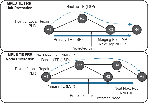
The decision of whether to use link protection or node protection, or both, is mainly based on the network architecture, physical topology layout, level of protection, and the ultimate goal to be achieved by the FRR. However, under general design principles, it is always recommended to keep it as simple as possible. For instance, consider protection for one failure rather than double failure scenarios to avoid situations where you design MPLS-TE FRR to cater for both link and node protection. In addition, if the network node has a reliability level of 99.999 percent, while the line cards or the interconnecting optical links have 99.5 percent of reliability, it is more reasonable to use link protection rather than node protection. Similarly, if a high level of end-to-end LSP availability is required and the next hop (NHOP) passes through an SRLG but the next-next hop (NNHOP) does not, it might be more feasible to use NNHOP to satisfy this design requirement. Again, these are only general design decision considerations. The actual decision has to be driven by the design requirements in terms of business requirements, functional requirements, and application requirements.
MPLS-TE FRR Design Considerations
In addition to the points highlighted with regard to the different approaches of MPLS-FRR, some technical considerations must be taken into account during the planning and design phases of any MPLS-TE FRR to achieve a successful and effective solution that can deliver its promised value. This section discusses the most common considerations with regard to MPLS-TE FRR design.
Multiple Backup Tunnels and Tunnel Selection
The only limiting factor for the maximum configurable number of backup tunnels to protect a given interface is memory limitations. However, the more tunnels and backup tunnels in the network, the more design and operational complexity is added to the network. Therefore, as a rule of thumb, it is always recommended to not overengineer the network with an extremely high number of MPLS-TE tunnels and backup tunnels (the same concept discussed earlier when having many redundant links will overweigh the benefits at higher layers, such as the network routing layer). Nonetheless, in some scenarios, having multiple TE back tunnels can be beneficial, such as the following:
![]() Additional redundant paths: It may be feasible to consider additional backup tunnels to protect the LSPs of critical traffic with a higher level of redundancy requirements, to cater for a double-failure scenario.
Additional redundant paths: It may be feasible to consider additional backup tunnels to protect the LSPs of critical traffic with a higher level of redundancy requirements, to cater for a double-failure scenario.
![]() Link capacity purposes: Sometimes the protected interface has a high bandwidth, whereas the alternate paths each individually cannot offer the same level of link capacity. Therefore, distributing the traffic over multiple backup tunnels can protect this high-capacity link over multiple paths (backup LSPs) to maintain adequate bandwidth protection following a failure event.
Link capacity purposes: Sometimes the protected interface has a high bandwidth, whereas the alternate paths each individually cannot offer the same level of link capacity. Therefore, distributing the traffic over multiple backup tunnels can protect this high-capacity link over multiple paths (backup LSPs) to maintain adequate bandwidth protection following a failure event.
For instance, if the protected interface is a high-capacity link and no single backup path exists with an equal capacity, multiple backup tunnels can protect that one high-capacity link. The LSPs using this link will fail over to different backup tunnels, allowing all the LSPs to have adequate bandwidth protection during failure (rerouting). In other words, if bandwidth protection is not desired, the router spreads LSPs across all available backup tunnels (load balancing across backup tunnels).
However, technically, if multiple backup tunnels are deployed, the backup tunnel selection process will consider the following selection criteria when choosing the preferred one:
![]() Tunnel that terminates at the NNHOP over a tunnel that terminates at NHOP.
Tunnel that terminates at the NNHOP over a tunnel that terminates at NHOP.
![]() Tunnel deployed with subpool reservation will be preferred over a tunnel deployed with any pool (same concept applies to tunnels delayed with global pool reservation, global pool over the one with any).
Tunnel deployed with subpool reservation will be preferred over a tunnel deployed with any pool (same concept applies to tunnels delayed with global pool reservation, global pool over the one with any).
![]() Tunnel deployed with the lowest sufficient subpool reservation will be preferred over a tunnel deployed with a higher bandwidth subpool reservation.
Tunnel deployed with the lowest sufficient subpool reservation will be preferred over a tunnel deployed with a higher bandwidth subpool reservation.
![]() Tunnel deployed with limited backup bandwidth over a tunnel deployed with unlimited bandwidth.
Tunnel deployed with limited backup bandwidth over a tunnel deployed with unlimited bandwidth.
For instance, in the scenario illustrated in Figure 9-10, if an LSP at R1 requires a backup tunnel with a 1-Mbp subpool bandwidth, the preferred tunnel will be selected based on the tunnel selection preferences previously listed, as follows:
1. TE2, TE3, and TE4 are first, because they all terminate at NNHOP.
2. TE2 will be eliminated because it protects only LSPs using global-pool bandwidth.
3. TE3 will be preferred over TE4 because it is deployed with a subpool that has the least sufficient backup bandwidth available as compared to TE4.
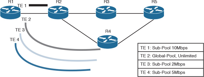
Therefore, to ensure that the protected traffic flows can be distributed across multiple backup TE tunnels, the attributes of the backup TE tunnels with regard to the selection criteria highlighted above must be the same.
Path Reoptimization and MPLS-TE Tunnel Promotion
One of the most common requirements with MPLS-TE with FRR is that traffic must reuse the original LSP/MPLS-TE tunnel after the failed link or node has recovered. Another common requirement is that MPLS-TE paths should be moved across links/paths that are less congested or optimal when they are available. From a high-level design point of view, both requirements are valid points and offer a value to the business (more optimized and dynamic paths and bandwidth utilization). However, two primary design concerns should be considered:
![]() Network stability: Moving traffic from one MPLS-TE tunnel to another in a matter of subseconds can impact network stability in some situations, such as when there is a link flap and traffic will keep moving between the primary and backup MPLS-TE tunnels.
Network stability: Moving traffic from one MPLS-TE tunnel to another in a matter of subseconds can impact network stability in some situations, such as when there is a link flap and traffic will keep moving between the primary and backup MPLS-TE tunnels.
![]() RSVP double booking of bandwidth: In each of the design requirements above, traffic has to be moved from one MPLS-TE tunnel to another. Ideally, traffic transition must be performed in a transparent manner in which no service interruption must occur (unnoticeable by applications). To achieve this MPLS-TE, use a principle called make before break (refer to IETF, RFC 3209).
RSVP double booking of bandwidth: In each of the design requirements above, traffic has to be moved from one MPLS-TE tunnel to another. Ideally, traffic transition must be performed in a transparent manner in which no service interruption must occur (unnoticeable by applications). To achieve this MPLS-TE, use a principle called make before break (refer to IETF, RFC 3209).
In addition, the conditions of MPLS-TE backup tunnels may change for any given LSP, in which case it will cause reevaluation or what is commonly known as promotion. Such scenarios include the following:
![]() A new backup tunnel comes up. For instance in Figure 9-11, the MPLS-TE tunnel 1 is protected by TE tunnel 20 (NHOP). When backup TE tunnel 30 (NNHOP) comes up on line, this may cause reevaluation of the current backup tunnel.
A new backup tunnel comes up. For instance in Figure 9-11, the MPLS-TE tunnel 1 is protected by TE tunnel 20 (NHOP). When backup TE tunnel 30 (NNHOP) comes up on line, this may cause reevaluation of the current backup tunnel.
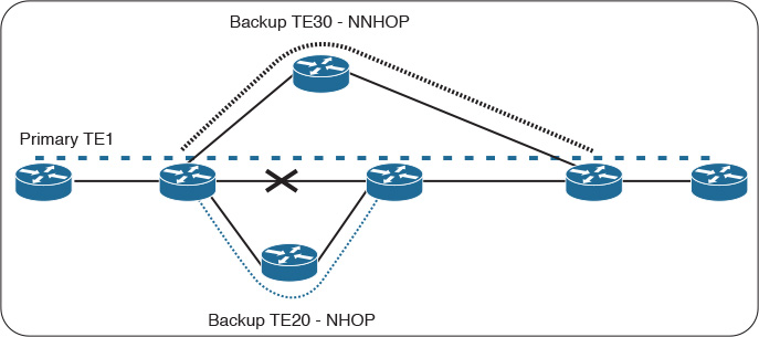
![]() The actual available bandwidth (or required bandwidth) for the current active backup tunnel may change.
The actual available bandwidth (or required bandwidth) for the current active backup tunnel may change.
![]() The current active backup tunnel may go down.
The current active backup tunnel may go down.
Note
Reevaluation of the current TE backup does not mean the protected LSP must switch over to a new path immediately. In other words, if an LSP is actively using a backup tunnel and a better backup tunnel becomes available, the active LSP is not switched to the better backup tunnel; instead, it might be considered during the next periodic promotion cycle [63].
Path Diversity and Fate Sharing
The main goal of FRR is to provide a precomputed backup path with an extremely fast switchover time from the primary (failed path) to the backup path. However, sometimes the backup path may traverse an SRLG point. This can introduce a risk for a certain type of traffic that must meet a tight SLA with a high degree of end-to-end path reliability and service availability. Therefore, network designers in scenarios like this should cater to a double-failure scenario and make sure that the backup TE tunnel takes a diverse path from the primary path. Network designers should also avoid any SRLG in the path (if possible) to avoid fate sharing during failure scenarios.
One of the main concerns with MPLS-TE and FRR is the scalability limitations when the network grows to an extremely large number of nodes due to the mesh nature of MPLS-TE. Therefore, a combined approach of MPLS-TE FRR and other FRR mechanisms, such as loop-free alternate (LFA), is sometimes used to lessen the impact of having a very large number of primary and backup tunnels across the network.
In addition, the location of the TE headend and tail end and how the backup tunnels handle the backup LSPs are primary influences on the level of scalability of the TE and FRR design (as highlighted earlier in Chapter 5) (in other words, if the TE tunnels are set up between PEs versus across the core only [P] routers and whether one backup tunnel is designed to protect multiple interfaces, where one backup tunnel can protect hundreds or thousands of LSPs [also known as N:1]. For example, using MPLS-TE FRR directly between PEs in a service provider network with tens or hundreds of PEs can significantly complicate the design and increase operational cost and control plane complexity.
The aforementioned points are purely design decisions. Practically, it is impossible to generalize and advise that a certain design option is almost always better. Yet by understanding the impact of these points on the overall network and FRR solution scalability, network designers can make a better design decision, considering the goals that need to be achieved, business priorities, network size, and the supported technologies and capabilities. For example, some networks may have a software code that does not support LFA, and a software upgrade is not an option. In this case, LFA will be eliminated from the design options. Similarly, if a service provider wants to meet certain levels of an SLA for its VIP customers, where no single point of failure must exist along the primary and backup paths, it is more feasible to set up MPLS-TE along with FRR end to end (PE-to-PE), which excludes any SRLG in the path that meets bandwidth and other constrained SPF (CSPF) requirements. As highlighted in Chapter 5, the planning of the MPLS-TE is crucial to generate a viable and reliable design, including FRR considerations.
Bandwidth Protection Considerations
Bandwidth protection with regard to MPLS-TE FRR back tunnels is one of the main design considerations that must be accounted for during the planning phase of the solution. From a design point of view, an MPLS-TE FRR design strategy that includes bandwidth protection offers a more reliable FRR solution. With this approach, the backup tunnel selection takes into consideration bandwidth availability over any given path. As a result, operators can satisfy strict SLA requirements. For example, delay-sensitive traffic, such as VoIP traffic riding a TE tunnel, can be protected with MPLS-TE FRR, which can avoid placing the backup TE tunnel over congested paths following a link or node failure. Bandwidth protection with MPLS-TE FRR commonly uses the following approaches:
![]() Limited bandwidth: With this approach, the LSPs must have a predefined bandwidth to be protected with an MPLS-TE backup tunnel. However, the aggregate value of the LSP’s bandwidth that needs to use the TE backup tunnel must not exceed the assigned bandwidth value of the TE backup tunnel. This approach is simple to deploy, but it may introduce limitations with regard to bandwidth sharing of MPLS-TE backup tunnels protecting different independent failures/LSPs.
Limited bandwidth: With this approach, the LSPs must have a predefined bandwidth to be protected with an MPLS-TE backup tunnel. However, the aggregate value of the LSP’s bandwidth that needs to use the TE backup tunnel must not exceed the assigned bandwidth value of the TE backup tunnel. This approach is simple to deploy, but it may introduce limitations with regard to bandwidth sharing of MPLS-TE backup tunnels protecting different independent failures/LSPs.
![]() Unlimited bandwidth: With this approach, the MPLS-TE backup tunnel does not provide any bandwidth protection, and the LSPs over this backup TE tunnel will share the same backup tunnel in a best effort fashion. However, only the MPLST-TE LSPs signaled with zero bandwidth can use the backup tunnels that have unlimited backup bandwidth. This approach offers a cost-effective (economical bandwidth usage) solution that supports oversubscription by sharing bandwidth protection used to cater for multiple independent failures. However, this approach does not offer differentiated treatment for different types of LSPs such as VoIP and data. Therefore, it is commonly used when MPLS-TE is intended to provide basic link protection only.
Unlimited bandwidth: With this approach, the MPLS-TE backup tunnel does not provide any bandwidth protection, and the LSPs over this backup TE tunnel will share the same backup tunnel in a best effort fashion. However, only the MPLST-TE LSPs signaled with zero bandwidth can use the backup tunnels that have unlimited backup bandwidth. This approach offers a cost-effective (economical bandwidth usage) solution that supports oversubscription by sharing bandwidth protection used to cater for multiple independent failures. However, this approach does not offer differentiated treatment for different types of LSPs such as VoIP and data. Therefore, it is commonly used when MPLS-TE is intended to provide basic link protection only.
Moreover, it is important to identify the backup protection strategy used, whether the protection is N:1 (facility) or 1:1. For instance, let’s assume that an N:1 MPLS-TE backup strategy is used (without DS-TE). This means a single backup tunnel is protecting multiple LSPs. If there is an LSP carrying VoIP (delay-sensitive traffic) while other LSPs carrying data, in this case, even though an explicit bandwidth is signaled for the backup tunnel, in the case of a failure all the LSPs crossing the link will be using the same backup TE tunnel, in which VoIP traffic will not get any priority over other tunnels for data traffic. This does not mean that VoIP will always suffer with this strategy because the backup path might be overprovisioned. However, it is more of a concern that the backup path may introduce congestion in a failure scenario.
Note
As mentioned earlier, when multiple TE backup tunnels are available with different bandwidth allocation models such as global pool, subpool, or no bandwidth limit, the TE backup tunnel selection will be impacted. Furthermore, the LSPs signaled with zero bandwidth might even be demoted. This “demotion” occurs when there are one or more LSPs (without the bandwidth protection bit set) to be removed from the current assigned TE backup tunnel to provide backup to an LSP that has its bandwidth protection bit set. This scenario happens when there is insufficient backup bandwidth.
Loop-Free Alternate Path (IP FRR)
The goal of IP FRR is to reduce failure reaction time to tens of milliseconds by applying the same concept of EIGRP feasible successor to link-state routing protocols. A precomputed loop-free alternate next hop is used if the currently selected primary next hop fails, as soon as the failure is detected. A network with this feature usually experiences less traffic loss and less microlooping of packets than a network without IP FRR [Loop-free Alternate IETF draft-ietf-rtgwg-ipfrr-spec-base-12], as illustrated in Figure 9-12.
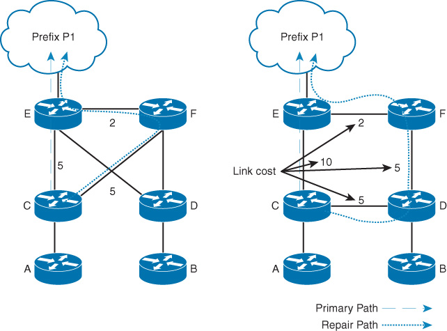
Note
In Figure 9-12 (square topology), the node D primary path to reach prefix P1 is via node F (lower path cost). Therefore, LFA is applicable in this topology (because forwarding traffic immediately after a C to E link failure will not impose any potential looping).
LFA usually offers per-prefix protection (fast convergence) for simple triangular topologies. Ring topologies, however, require considerations of the other flavor of LFA, known as remote LFA. In remote LFA, the headend node uses a tunneling mechanism (typical LDP based) to configure an MPLS path. This alternate path is installed as an LFA in the Cisco Express Forwarding (CEF) table. As a result, the LFA can bring the overconvergence time in the supported topologies to less than 50 ms after the detection of the failure because the protocol does not need to wait for the failure propagation, processing, and SPF calculation. Instead, the node can switch over quickly to the precomputed alternate path within a few milliseconds.
Despite the fact the LFA offers simple and native IP FRR support with link-state routing protocols, the following limitations, in which LFA may not be an optimal solution for every design, must be considered:
![]() LFA consumes hardware resources, which makes it less than ideal when there are many interconnections between the network nodes, such as with partially meshed and fully meshed topologies, in addition to the added complexity if LFA is in these types of topologies.
LFA consumes hardware resources, which makes it less than ideal when there are many interconnections between the network nodes, such as with partially meshed and fully meshed topologies, in addition to the added complexity if LFA is in these types of topologies.
![]() LFA is limited within a single IGP flooding domain.
LFA is limited within a single IGP flooding domain.
![]() Ring and some square topologies require packets tunneling such as MPLS to be enabled for the remote LFA to establish an LDP session, as illustrated in Figure 9-13.
Ring and some square topologies require packets tunneling such as MPLS to be enabled for the remote LFA to establish an LDP session, as illustrated in Figure 9-13.
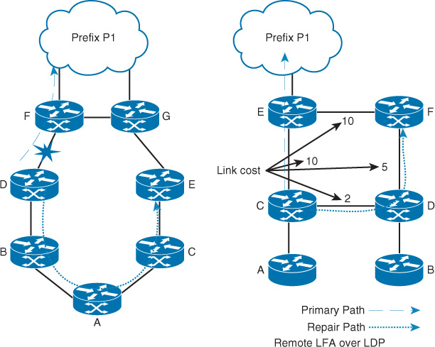
Note
By comparing the square topology in Figure 9-13 to the one illustrated in Figure 9-12, it is obvious that in Figure 9-13 node D’s preferred path to reach prefix P1 is via node C. Therefore, remote LFA R-LFA (with LDP encapsulation) is required to avoid any microlooping following C to E link failure.
The decision whether to use LFA needs to be made with input from network designers about the topology, to what extent the solution has to be deterministic, and the required FRR coverage; for example, in an SP environment across the edge networks only (points of presence [POP]), core, or both. Practically, LFA is more applicable to POP design, in particular to the ones designed in triangles. It can offer a fully protected LFA solution against both link and node failures compared to the square topology, where some prefixes may not offer a full LFA without considering the remote LFA concept.
The core of the network, however, might not be as simple and common as with the POPs. For instance, the underlying physical topology can influence the decision of whether LFA applies. Redesigning a POP network topology is almost always easier, cheaper, and less disruptive than redesigning a core network. Therefore, if the core topology is not fully supported by LFA or the network designer aims to achieve a more precise and deterministic path protection mechanism, MPLS-TE can be a better choice here. These issues will drive us to ask the question: LFA versus MPL-TE: Which one is better? Table 9-3 compares both solutions from different design aspects. Based on the scenario, requirements, and design constraints, network designs can select the most suitable approach.
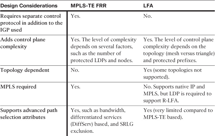
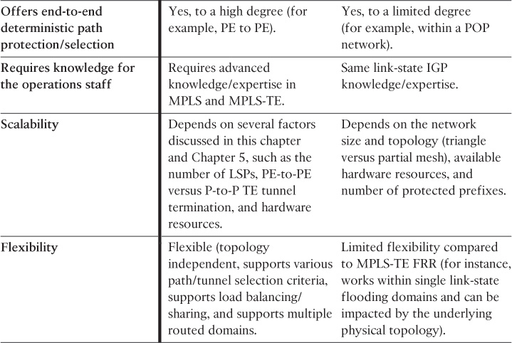
Like the MPLS-TE planning approaches discussed in Chapter 5, LFA is no different here. Network designers must
![]() Assess the goal of the solution (for example, only path protection or provide differentiated services with path protection)
Assess the goal of the solution (for example, only path protection or provide differentiated services with path protection)
![]() Assess the current environment in terms of
Assess the current environment in terms of
![]() Routing protocol in use
Routing protocol in use
![]() Physical topology.
Physical topology.
![]() Native IP or MPLS based
Native IP or MPLS based
![]() Single or multiple routing (flooding) domains
Single or multiple routing (flooding) domains
![]() Level of flexibility (for example, how flexible and easy it is for this topology to be altered or redesigned [based on the situation])
Level of flexibility (for example, how flexible and easy it is for this topology to be altered or redesigned [based on the situation])
After this foundational information has been identified, network designers can make the call whether to use LFA, MPLS-TE, or a combination of both, considering the design aspect listed in Table 9-3.
For instance, an MPLS VPN service provider with the network architecture depicted in Figure 9-14 requires very low network convergence time (path protection) across the entire network and highly flexible with advanced path protection capabilities across the core without any requirement of service differentiation. Also the suggested solution should cater for ease of deployment requirements of this operator.
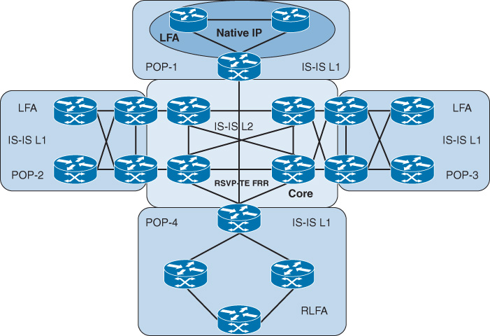
Based on the requirements provided and the network architecture, it is feasible to use LFA at the edge of the network (single flooding domain, no additional protocol to design and manage and no physical connectivity change required at the POP or core levels), while one-hop MPLS-TE along with autotunnel backup MPLS-TE FRR can be applied at the core of the network, which provides path protection that offers advanced TE capabilities without being impacted by the underlying physical connectivity (full mesh in this scenario) and with minimal operational efforts. For more details, refer to the “Further Reading” list at the end of this chapter.
BGP FRR
BGP fast reroute (FRR) accelerates BGP convergence time significantly to minimize packet loss and to avoid traffic black-holing situations after a failure event when IGP is tuned to converge in a subsecond, without sacrificing network stability. The BGP FRR concept enables BGP to use alternate paths within a subsecond following a failure event of the current active path. BGP FRR is achieved through BGP prefix-independent convergence (PIC) concept, where BGP installs a backup path or paths in RIB/FIB tables that are ready for immediate use. Therefore, a more predictable and constant convergence time of BGP can be achieved no matter how large the number of BGP prefixes is.
For example, in the MPLS VPN scenario in Figure 9-15, PE1 always considers PE2 as the preferred MP-iBGP next-hop to reach AS 600 prefixes. However, with BGP PIC, PE1 also installs an alternate path in its RIB/FIB tables (P4 in this example). When PE2 fails, PE1 will be aware of this event through the removal of the host prefix by IGPs in subsecond (assuming IGP is tuned to converge in subsecond) and will start to redirect traffic toward the alternate next-hop (via PE4). In the meantime the standard BGP convergence can take place while BGP PIC is forwarding the traffic through PE4 without introducing packet loss (or it will be very minimal, if there is any). As a result, BGP PIC offers more structured RIB/FIB tables (at the core or edge of the network) that helps network designers to align with the underlying IGP fast convergence as well as minimize packet loss and network instability following any network component failure.
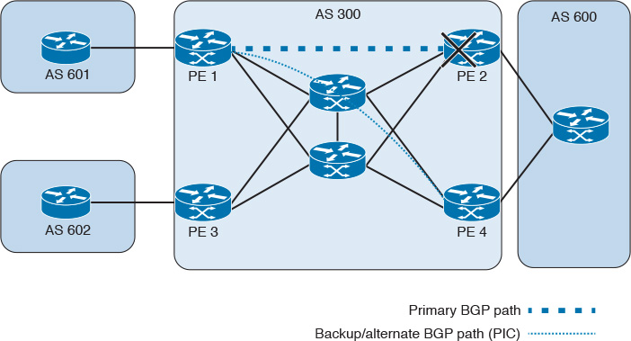
Similarly, BGP PIC offers more structured RIB/FIB tables that helps to achieve faster network convergence and minimize packets loss at the edge of the network, usually in an SP-style environment following a PE-CE link failure for multihomed CE sites. For instance, AS 600 in Figure 9-16 can be protected with BGP PIC to achieve BGP FRR using the same concept discussed earlier, where PE2 holds primary and backup paths (primary via the directly connected PE-CE link and the backup via PE4 best external). As soon as PE2 detects the link to AS 600 CE failure, traffic will be shunted to PE4 to reach the AD 600 CE to avoid packet loss, while BGP will continue its typical route withdrawal and update propagation to converge the network, as illustrated in Figure 9-16. However, because PE-CE communication is normally over an external BGP (eBGP) session (no IGP to react to the failure and updated RIB/FIB), bidirectional forwarding detection (BFD) is required to detect a failure of an eBGP one-hop peer in less than a second. This can be combined with the BGP failover feature to track the availability of the BGP neighbor (CE), not only based on link status.
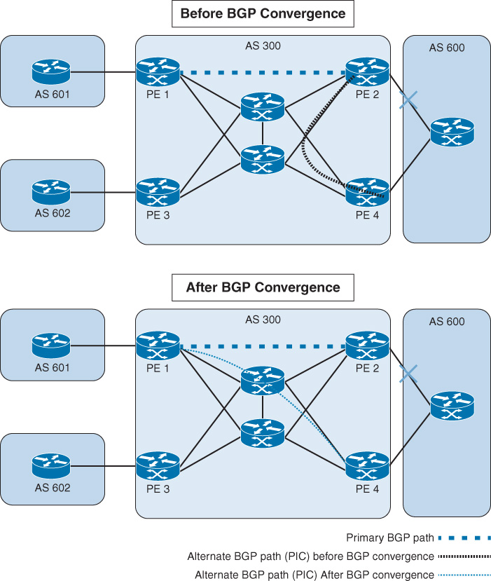
Note
Typically, at the FIB level, after a failure event where a next hop to a prefix fails, the FIB (Cisco CEF) will look for another path to reach the same prefix by searching through the FIB table to find the next longest matching path to the prefix. This proves beneficial when the next hop is several hops away and there are multiple paths to reaching that next hop, such as a router with a loopback interface IP address that is reachable via multiple physical interfaces/paths. However, this feature (recursion) may impact and conflict with the BGP PIC concept, because there is a precomputed alternate path already in place with BGP PIC. Moreover, the searching process through the FIB table almost always slows down convergence time in general. Therefore, ideally, the CEF recursion feature should be disabled at least for the learned host routes when BGP PIC is in use. In some Cisco platforms, “When the BGP PIC functionality is enabled, Cisco Express Forwarding recursion is disabled by default for next hops learned with /32 host routes and next hops that are directly connected.”4
4. “BGP PIC Edge for IP and MPLS-VPN,” http://www.cisco.com
BGP Multiple Path Announcement Solutions
The natural behavior of BGP, as defined in RFC 4271, is to announce only a single path to its BGP neighbors, known as the BGP best path. However, in some scenarios, the announcement of multiple paths within BGP is becoming a requirement, especially when BGP fast convergence is required. Furthermore, BGP path hiding of BGP RRs may prevent the efficient use of BGP multipath or keep BGP PIC from working properly. BGP path hiding also inhibits fast and local recovery because the network has to wait for the standard BGP control plane convergence to restore traffic across the network [34]. Therefore, a solution that offers path diversity is required for networks that need to use the available path or need to maintain a fast network convergence at the control plane level (BGP). Multiple solutions are available to change this default behavior of BGP and facilitate the ability to advertise multiple paths with BGP, some of which were already discussed in Chapter 5 with regard to hot-potato routing with RR. In addition, these mechanisms serve to optimize BGP FRR in similar scenarios:
![]() BGP additional paths
BGP additional paths
![]() BGP best external
BGP best external
![]() BGP diverse paths
BGP diverse paths
![]() Different route distinguisher (RD) approach with MP-BGP in MPLS VPN environments
Different route distinguisher (RD) approach with MP-BGP in MPLS VPN environments
Summary
This chapter covered high-availability network design and the primary elements and approaches to achieve it at multiple layers. This chapter also discussed how the concept of network convergence consists of multiple elements that all collectively work together to achieve the overall desired convergence time. In addition, two primary approaches at the protocol level (the network protection approach and the network recovery approach) to achieve the desired level of network resiliency were also examined, with each having advantages and limitations, as summarized in Table 9-4.
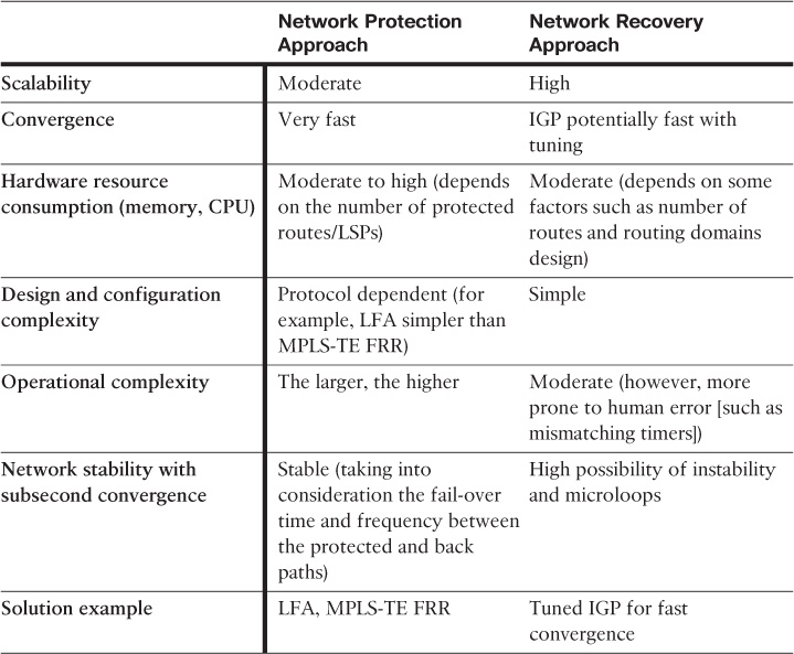
Last but not least, this chapter explained, in multiple places, that the level of availability will vary from network to network and from part to part within the same network, based on multiple variables and mainly driven by the application criticality and business priorities. In other words, not every network or every part of the network needs HA considerations or fast network convergence. For network designers to identify when and where to consider it, a good understanding of the application, functional, and business requirements is required. (For instance, identify what is critical and high priority to the business, versus what is important but not high priority, versus what is not critical and not high priority.)
Further Reading
“High Availability Campus Recovery Analysis Design Guide,” http://www.cisco.com
RFC 6571, Loop-Free Alternate (LFA) Applicability in Service Provider (SP) Networks, http://www.ietf.org
“Remote Loop-Free Alternate (LFA) Fast Re-Route (FRR),” draft-ietf-rtgwg-remote-lfa-11, http://www.ietf.org
RFC 6413, Benchmarking Methodology for Link-State IGP Data-Plane Route Convergence, http://www.ietf.org
RFC 4090, Fast Reroute Extensions to RSVP-TE for LSP Tunnels, http://www.ietf.org
“MPLS Traffic Engineering (TE) - Autotunnel Primary and Backup,” http://www.cisco.com
“Redundancy Mechanisms for Carrier Ethernet Networks and Layer 2 VPN Services,” http://www.ciscolive.com
RFC 6981, A Framework for IP and MPLS Fast Reroute Using Not-Via Addresses, http://www.ietf.org