Chapter 7
WLAN Media and Application Services
Introduction
Providing differentiated treatment for different types of applications is a difficult challenge for Wi-Fi networks (and CCIE candidates). Wi-Fi networks are inherently unstable. Speeds are half duplex, overhead renders the links less deterministic, devices move, and users tend to bring old devices that disrupt the performance of your latest shiny fast phone or laptop.
In this context, providing a good application experience for your users requires a combination of sound RF design, a good understanding of your client database, and a solid background in QoS foundations and QoS configuration. This last aspect is difficult to acquire because you will find that, in AireOS, QoS features that saw light in the early days of Wi-Fi QoS (and are now nearly obsolete) stand next to QoS features that just appeared in the 802.11 standard. This chapter will help you triage all these elements and give you the basis you need to provide a good quality experience to your users. You should also be able to face the exam in confidence. This chapter is organized into two sections. The first section gives you the technical background you need to understand application differentiated services over Wi-Fi. The second section shows you how these elements are configured on the various platforms, AireOS, switches, and Autonomous APs. More specifically, the two sections are organized as follows:
Section 1 provides the survival concepts needed to understand QoS over 802.11. This section first introduces the notion of differentiated services to help you understand DSCP markings and IP Precedence. These notions are then related to QoS design and the concept of traffic classes. Operating QoS classes implies recognizing traffic, and the following subsections explain how traffic is identified and marked, with Layer 3 techniques for IPv4 and IPv6, and with Layer 2 techniques, with 802.11e and also 802.1Q, 802.1D, and 802.1p, to which 802.11e often gets compared. This first section then examines different techniques to handle congestion.
Section 2 covers the configuration of differentiated treatment for application services over the various architectures. The first architecture to be covered is AireOS, and you will see how QoS profiles, bandwidth contracts, QoS mappings, and trust elements are configured. You also learn how to configure congestion management techniques, including EDCA parameters, CAC, and AVC. You then see how Fastlane creates specific additions for iOS and MacOS devices. You then learn how application services are configured for autonomous APs. Quite a few items available on AireOS are also configured on autonomous APs; however, autonomous APs are Layer 2 objects. Therefore, they present some variations that you need to understand and master. Finally, you will see how QoS is configured on switches. Your goal is not to become a QoS expert but to be able to autonomously configure a switch to provide a basic support for the QoS policies you configured on your WLAN infrastructure.
At the end of this chapter, you should have a good understanding of real-time application support for wireless clients.
QoS Survival Concepts for Wireless Experts
QoS is not a static set of configuration commands designed long ago by a circle of wise network gurus and that are valid forever. In fact, QoS models, traffic definitions, and recommendations have evolved over the years as common traffic mixes in enterprise networks have changed. With new objects (such as IoT), new protocols, and new traffic types, QoS continues to evolve. However, you do not need to be a QoS expert to pass the CCIE Wireless exam, you just need to understand the logic of QoS and survive by your own, configuring standard QoS parameters that will affect your Wi-Fi network’s most sensitive traffic (typically Voice). In short, your task is to understand QoS well enough to make Voice over Wi-Fi work.
The Notion of Differentiated Treatment
Let’s start with a quiz question: What is the second most configured feature in Cisco networking devices? If you read the title of this chapter, then you probably guessed: QoS (the first one is routing).
QoS is therefore a fundamental concept. However, to help you survive the complexities of the CCIE lab exam, but also to help you face real deployment use cases, we need to dispel a few legends. The first legend is that QoS is about lack of bandwidth and that adding bandwidth solves the problem and removes the need for QoS. This is deeply untrue. QoS is about balance between the incoming quantity of bits per second and the practical limitations of the link where these bits must be sent.
Let’s look at a nonwireless example to help clarify this concept. Suppose that you need to send a video flow over a 1 Gbps switch interface. The communicated bandwidth, 1 Gbps, is only an approximation over time of the capacity of the link. One gigabit per second is the measure of the transmission capability of the Ethernet port and its associated cable (over 1 second, this port can transmit one billion bits). But behind the port resides a buffer (in fact probably more than one, each buffer being allocated to a type of traffic), whose job is to store the incoming bits until they can be sent on the line, and a scheduler, whose job is to send blocks of bits to the cable.
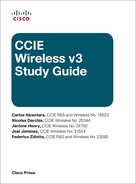
A high-end switch buffer can store 5.4 MB. If the switch port is built around the notion of four queues, that’s 1.35 MB per queue. Now, your port can send 1 gigabit per second, which translates to about 125 kilobytes per microseconds. If you map the buffer to the link speed, you see that the buffer can store up to 10.8 ms of data before being filled up.
Suppose that your switch receives a flow of video packets, representing a modest 2 MB burst intended to draw a full 32-color 1080p video frame. You can immediately see that, even if the port is completely idle before the burst arrives from within the switch bus (let’s assume that the internal bus is faster than 1 Gbps; a common speed for a good switch can be around 480 Gbps), the buffer can saturate long before the entire flow is stored and then transmitted on the line, as shown in Figure 7-1.
From the outside, you see a modest 2 MB burst of packets, a very low link utilization (less than 1%), and yet several bytes are dropped. The issue is that 2 MB should never have been sent to that queue in less than 11 ms, and this is where QoS comes into play. Here, more bandwidth does not solve the problem (you already have enough bandwidth, and your link utilization is overall less than 1%). What solves the problem is making sure that the right quantity of packets gets through the interface buffer in a reasonable amount of time, so as not to saturate the interface beyond capacity.
The same issue can be seen in the wireless world. Suppose that you send voice packets, using no QoS (best effort) from a smartphone to an access point. These packets are very small (one audio payload can typically represent 160 bytes), so bandwidth is typically a non-issue. Yet, oblivious to the presence of voice traffic (as you use best effort), the AP suddenly jumps to another channel to scan (RRM). The AP is likely to be gone for about 80 ms, during which your phone will fail to receive an ACK for the last voice packet, will retry many times while rate shifting down, then drop the packet and attempt to send the next one, and so on. When the AP returns to the channel, you will have lost three consecutive packets, which is enough for the user to detect a short drop in the audio flow and complain about Wi-Fi. Yet, troubleshooting the issue will show no oversubscription of the link. The issue is not bandwidth. The issue is that proper priority was not given to this real-time traffic over other tasks. Typically, 30 ms in the cell is the maximum time interval allowed for a Wi-Fi driver to send a real-time voice frame (UP 6). After that delay, this type of frame is dropped from the queue. Here again, the solution is not more bandwidth but proper servicing over time of packets based on their specific category. In other words, ensure that voice packets are not delayed for more than 30 ms in the cell, regardless of the available bandwidth. This is again what QoS does.
Another lasting legend about QoS is that it should be configured on weak links (typically, WAN and Wi-Fi). However, QoS is not a Wi-Fi or a WAN problem—it is an end-to-end problem. Each medium has unique characteristics, and the complexity of configuring QoS is to make sure to translate the requirements of each traffic type into configurations adapted to the local medium. Therefore, you need a mix of global configurations and local particulars to express a global QoS intent for each traffic and translate this intent to each local medium specific constraints. As you saw from the bandwidth urban legend, your Wi-Fi could be configured for QoS and yet traffic could be dropped on the switch side, if you neglected the LAN side because of its large bandwidth.
This end-to-end concern, and also the fact that Wi-Fi is one of the weakest links, are the reasons why the CCIE Wireless exam expects from you the ability to configure QoS for Wi-Fi but also have reasonable knowledge on how the intent you expressed through your Wi-Fi QoS configuration would translate on the switch port to your access point or your WLC. You do not need to be a QoS expert, but you must be able to verify that QoS will not stop at the AP or WLC port. This ability translates into the knowledge of the different families of traffic and the various possibilities brought by QoS to offer a different treatment for different types of traffic: prioritize urgent business-relevant traffic and delay or drop traffic of lower urgency or importance depending on the link capacity.
Traditionally, these requirements translate into different possible types of actions and mechanisms:
QoS Design: Your first task is to determine which traffic matters for your network. Most of the time, this determination will bring you to create different categories of traffic.
Classification and marking: After traffic starts flowing and enters your network, you must identify it; when identification is completed, you may want to put a tag on each identified traffic packet so as not to have to run the identification task at every node.
Congestion management tools: When congestion occurs, multiple tools can help manage the available bandwidth for the best. In traditional QoS books, this section would cover many subsections, such as Call Admission Control mechanisms, policing, shaping, queue management, and a few others. In the context of the CCIE Wireless exam, you need to understand the main principles, and we will group under this category topics that matter for you.
Link efficiency mechanisms: On some links, you can compress or simplify packets to send the same amount of information using less bandwidth. This is especially important on WAN connections but is completely absent from Wi-Fi links. You will find efficiency mechanisms for Wi-Fi, such as MIMO, blocks, and a few others, and they do improve transmissions. However, this is not efficiency in the sense of transmission compression or simplification. The term link efficiency is important to know in the context of QoS, but you will not need to implement such a mechanism, with a QoS approach, for Wi-Fi.
The listed actions and mechanisms have different relative importance for the CCIE Wireless exam. The following sections cover what you need to know, and we refer to the category names along the way to help your learning.
QoS Design
Just as you do not start building a house without a blueprint, you also do not start configuring QoS without a QoS blueprint. This blueprint lists the types of traffic that you expect in your network and organizes these types into categories. As a Wireless CCIE, your job is not to build an enterprise QoS blueprint. However, a basic understanding of what this blueprint covers will help you reconcile the apparent inconsistencies between 802.11e QoS marking and DSCP/802.1p marking, and will also show you why some vendors get it right and others do not.
The main concern behind this QoS blueprint, often called a QoS model, is about arbitration between packets. Suppose you have two packets that get onto an interface (toward any type of medium). Suppose that you have to decide which packet to send first (because your outgoing medium has a slower data rate than wherever these two packets came from), or you have to decide to pick one to send and drop the other (because your interface buffer cannot store the second packet, and because the second packet will not be useful anymore if it is delayed, or for any other reason). If you have built a QoS model, and if you know which packet belongs to which class in that model, you can make a reasonable choice for each packet.
A very basic QoS model runs around four classes: real-time traffic (voice or real-time conferencing), control traffic for these real-time flows (but this category also includes your network control traffic, such as RIP updates), data, and everything else. Data is often called transactional data, and it matches specific data traffic that you identified as business relevant and that you care about, such as database traffic, email, FTP, backups, and the like. Everything else represents all other traffic that may or may not be business relevant. If it is business relevant, it is not important enough that it needed to be identified in the transactional data category.
The four-queue model is simple and matches the switching queuing structure available in old switches (and vice versa; the switches queues were built to match the common QoS model implemented by most networks). This model was common 15 years ago, but it proved a bit too simple and over the years was replaced by a more complex 8-class model. Keep in mind that this was during the 2000s (you will see in a few pages why this is important).
The 8-class model separates real-time voice from real-time video. One main reason is that video conferencing increased in importance during these years. If you happen to use video conferencing, you probably notice that the sound is more important than the image. If your boss tells you that you are “…ired,” you want to know if the word was hired or fired. Sound is critical. However, if your boss’s face appears to pixilate for a second, the impact on the call is lower. Also, real-time video is video conferencing, and the 4-class model did not have a space for streaming video. It is different from transactional data because it is almost real-time, but you can buffer a bit of it. By contrast, video conferencing cannot be buffered because it is real-time.
Similarly, network control updates (like RIP or EIGRP updates) are not the same as real-time application signaling. As you will see in the next section, real-time application signaling provides statistical information about the call. It is useful to know if, and how, the call should be maintained. You can drop a few of these statistical packets without many consequences. Of course, if you drop too many of these packets, the call will suffer (but only one call will suffer). By contrast, if you drop EIGRP updates, your entire network collapses. The impact is very different, and putting both in the same control category was too simplistic.
Finally, there is clearly all the rest of the traffic, but there is also a category of traffic that you know does not matter. A typical example is peer-to-peer downloads (such as BitTorrent). In most networks, you want to either drop that traffic or make sure that it is sent only if nothing else is in the pipe. This traffic is called scavenger and should not compete with any other form of traffic, even the “Everything else” traffic that may or may not be business relevant.
The result is that the 8-class model implements the following categories: Voice, Interactive Video, Streaming Video, Network Control, (real-time traffic) Signaling, Transactional Data, Best Effort, and Scavenger.
The 8-class model is implemented in many networks. In the past decade, another subtler model started to gain traction, which further breaks down these eight classes. For example, the Network Control class is divided in two, with the idea that you may have some network control traffic that is relevant only locally, whereas some other network control traffic is valid across multiple sections of your network. Similarly, real-time video can be one way (broadcast video of your CEO’s quarterly update) or two ways (video conferencing). Usually, the broadcast is seen as more sensitive to delay and losses than the two-way video because the broadcast impacts multiple receivers (whereas an issue in a video-conference packet usually impacts only one receiver). Also, some traffic may be real time but not video (such as gaming). With the same splitting logic, a single Transactional Data category came to be seen as too simple. There is indeed the transactional data traffic, but if there is a transaction, traffic like FTP or TFTP does not fit well in that logic. Transactional should be a type of traffic where a user requests something from a server and the server sends it (ERP applications or credit card transactions, for example). By contrast, traffic such as file transfers or emails is different. This type of traffic can be delayed more than the real transactional data traffic and can send more traffic too, so it should have its own category. In fact, it should be named bulk data. In the middle (between the transactional data and the bulk data classes), there is all the rest, which is business-relevant data that implies data transfer but is neither transactional nor bulk. Typically, this would be your management traffic, where you upload configs, code updates, your telnet to machines, and the like. This class is rightly called Network Management (or Operations, Administration and Maintenance, or OAM).
This further split results in a 12-class model, with the following categories:
Network Control and Internetwork Control
VoIP
Broadcast Video
Multimedia Conferencing
Real-time Interactive
Multimedia Streaming
Signaling
Transactional Data
Network Management (OAM)
Bulk Data
Best Effort
Scavenger
A great document to learn more about these categories (and, as you will see in the DSCP part, their recommended marking) is the IETF RFC 4594 (https://www.ietf.org/rfc/rfc4594.txt).
Keep in mind that there is not a “right” QoS model. It all depends on what traffic you expect in your network, how granular you want your categorization to be, and of course, what you can do with these classes. If your switches and routers have only four queues (we’ll talk about your WLC and APs soon), having a 12-class model is great, but probably not very useful. You may be able to use your 12 classes in a PowerPoint but not in your real network.
In most networks, though, starting from a 12-class model allows the QoS designers to have fine-grained categories that match most types of traffic expected in a modern network. When some network devices cannot accommodate 12 categories, it is always possible to group categories into common buckets.
Application Visibility and Identification
Although QoS design should be your first action, it implies a knowledge of QoS mechanisms and categories. It is therefore useful to dwell on classification fundamentals, especially because Wi-Fi has a heavy history in the classification field.
Classifying packets implies that you can identify the passing traffic. The highest classification level resides at the application layer. Each application opens a certain number of sockets in the client operating system to send traffic through the network. These sockets have different relative importance for the performances of the application itself.
An example will help you grasp the principles. Take a voice application like Jabber. When the application runs, your smartphone microphone records the room audio, including (hopefully) the sound of your voice. Typically, such an application splits the audio into small chunks, for example, of 20 milliseconds each.
Note
You will find that there can be a lot of complexity behind this process, and that the process described here is not strictly valid for all applications. For example, some applications may slice time in chunks of 20 ms but record only a 10-millisecond sample over that interval, and consider it a good-enough representation of the overall 20 millisecond sound. Other applications will use 8 or 10 millisecond slices, for example.
Each 20-millisecond audio sample is converted into bits. The conversion process uses what is called a codec (to “code” and “decode”). Each codec results in different quantities of bits for the same audio sample. In general, codecs that generate more bits also render a sound with more nuances than codecs with a smaller bit encoding. A well-known reference codec is G.711, which generates about 160 bytes (1280 bits) of payload for each 20 ms sound sample. With 50 samples per second, this codec consumes 64 kbps, to which you must add the overhead of all the headers (L2, L3, L4) for the payload transmission. Other codecs, like PDC-EFR, consume only 8 kbps, at the price of a less-nuanced representation of the captured audio. It is said to be more “compressed” than G.711. Some codecs are also called elastic, in that they react to congestion by increasing the compression temporarily. The art of compressing as much as possible, while still rendering a sound with a lot of nuances, is a very active field of research, but you do not need to be a codec expert to pass the CCIE Wireless exam.
As you use Jabber, the application opens a network socket to send the flow of audio to the network. Keep in mind that the audio side of the application is different from the transmission side of your smartphone. Your network buffer receives from the application 160 bytes every 20 ms. However, transmitting one audio frame over an 802.11n or 802.11ac network can take as little as a few hundred microseconds. The function of the network stack is to empty the buffer, regardless of the number of packets present. When your Wi-Fi card gains access to the medium, it sends one block or multiple frames, depending on the operating system’s internal network transmission algorithm, until the buffer is empty. As soon as a new packet gets into the network buffer, the driver reattempts to access the medium, and will continue transmitting until the buffer is empty again.
Therefore, there is no direct relationship between the voice part of the application and the network part. Your smartphone does not need 1 second to send 1 second worth of audio, and your smartphone also does not need to access the medium strictly every 20 milliseconds. The application will apply a timestamp on every packet. On the receiver side, the application will make sure that packets are decoded back into a sound and played in order at the right time and pace (based on each packet timestamp).
The receiver will also send, at intervals, statistics back to the sender to inform it about which packets were lost, which were delayed, and so on. These statistic messages are less important than the audio itself but are still useful for the sender to determine, for example, whether the call can continue or whether the transmission has degraded beyond repair (in which case the call is automatically terminated). Sending such statistics implies opening another socket through the operating system. It is common to see real-time voice sent over UDP while the statistics part would be sent over a TCP socket. In a normal audio call, both sides exchange sounds, and therefore both sides run the previous processes.
Note
Some codecs use Voice Activity Detection, or VAD. When the microphone captures silence, or audio below a target volume threshold, the application decides that there is nothing to send and does not generate any packet for that sampling interval. However, this mechanism sometimes gives the uncomfortable impression of “dead air” to the listener. Many codecs prefer to send the faint sound instead. Others send a simplified (shorter) message that instructs the application on the listener’s end to play instead a preconfigured “reassuring white noise” for that time interval.
Many well-known applications can be recognized by the ports they use. For example, TCP 80 is the signature of web traffic. This identification is more complex for real-time applications because they commonly use a random port in a range. For example, Jabber Audio, like many other real-time voice applications, uses a random UDP port between 16384 and 32766. The port can change from one call to the next. This randomness helps ensure that two calls on the same site would not use the same port (which can lead to confusion when devices renew or change their IP addresses) and improves the privacy of the calls by making port prediction more difficult for an eavesdropper.
Processes like Network Based Application Recognition (NBAR, which is now implementing its second generation and is therefore often called NBAR2) can use the ports to identify applications. When the port is not usable, the process can look at the packet pattern (packet size, frequency, and the like) to identify the application. Looking beyond the port is called Deep Packet Inspection (DPI). NBAR2 can identify close to 1,400 different applications. Identification can rely on specific markers. For example, a client opening a specific (random) port to query a Cisco Spark server in the cloud then receives an answer containing an IP address, and then exchanges packets over the same port with that IP address, is likely to have just opened a Spark call to that address. NBAR2 can easily identify this pattern. When the whole exchange is encrypted, NBAR2 can rely on the packet flow (how many packets, of what size, at what interval) to fingerprint specific applications. NBAR2 can recognize more than 170 encrypted applications with this mechanism.
Therefore, deploying NBAR2 at the edge of your network can help you identify which application is sending traffic. However, running DPI can be CPU intensive. After you have identified the type of traffic carried by each packet, you may want to mark this packet with a traffic identifier so as not to have to rerun the same DPI task on the next networking device but apply prioritization rules instead. In some cases, you can also trust the endpoint (your wireless client for example) to mark each packet directly.
This notion of “trust” will come back in the “trust boundary” discussion, where you will decide whether you want to trust (or not) your clients’ marking.
Layer 3, Layer 2 QoS
Each packet can be marked with a label that identifies the type of traffic that it carries. Both Layer 3 headers (IPv4 and IPv6) and most media Layer 2 headers (including Ethernet and 802.11) allow for such a label. However, Layer 2 headers get removed when a packet transits from one medium to the other. This is true when a packet goes through a router. The router strips Layer 2 off, looks up the destination IP address, finds the best interface to forward this packet, then builds the Layer 2 header that matches that next interface medium type before sending (serializing) the packet onto the medium.
This Layer 2 removal also happens without a router. When your autonomous AP receives an 802.11 frame, it strips off the 802.11 header and replaces it with an 802.3 header before sending it to the Ethernet interface. When the AP is managed by a controller, the AP encapsulates the entire 802.11 frame into CAPWAP and sends it to the WLC. The WLC looks at the interface where the packet should be sent and then removes the 802.11 header to replace it (most likely) with an 802.3 header before sending it out.
In all cases, the original Layer 2 header is removed. For this reason, we say that the Layer 2 header is only locally significant (it is valid only for the local medium, with its specific characteristics and constraints). By contrast, the Layer 3 part of the packet is globally significant (it exists throughout the entire packet journey). This is true for the entire header, but is also true for the QoS part of that header. As a consequence, the QoS label positioned in the Layer 3 section of the packet expresses the global QoS intent—that is to say a view, valid across the entire journey, on what this packet represents (from a QoS standpoint). The label expresses a classification (what type of traffic this packet carries). Because your network carries multiple types of traffic (organized in categories, as detailed in the next section), each label represents a type of traffic but also expresses the relative importance of this traffic compared to the others. For example, if your network includes five traffic categories labeled 1 to 5, and if 5 is the most important category, any packet labeled 5 will be seen as not just “category 5” but also “most important traffic.” However, keep in mind that the label you see is “5,” and nothing else. You need a mapping mechanism to translate this (quantitative) number into a qualitative meaning (“most important traffic”).
The way Layer 3 QoS is expressed depends on the IP system you use (IPv4 or IPv6) and the tagging system you use (for example, IP Precedence or DSCP). Luckily, they are similar and inclusive of one another.
IPv4 QoS Marking
The IPv4 header has a field called Type of Service (ToS).
Note
Do not confuse Layer 3 Type of Service (ToS) and Layer 2 (e.g. 802.1) Class of Service (CoS). CoS is Layer 2, ToS is Layer 3. A way to remember it is to say that ToS is on Top, while CoS is Closer to the cable.
Using ToS, QoS can be expressed in two ways:
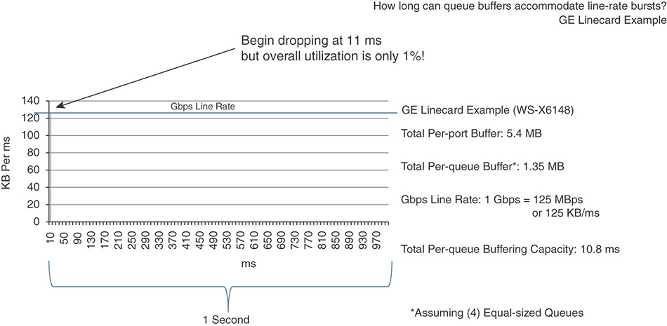
Three bits can be used to mark the QoS value. This is the IP Precedence system. You must be aware of its existence, but the next system (DSCP) incorporates IP Precedence. In most networks, IP Precedence is used only to express a QoS label compatible with other systems that also only allow 3 bits to express QoS (for example, 802.1 or 802.11). The IPv4 ToS field contains 8 bits. When IP Precedence is used, only the most significant bits (MSB, the bits on the left side) are used, resulting in a labeling scale from 000 to 111 (0 to 7 in decimal). The other bits (on the right) are usually left to be 0, although they can in theory be used to express other information, such as reliability or delay.
Another system, differentiated services code point (DSCP), extends the number of possibilities. DSCP uses the 6 bits on the left, thus creating 64 different QoS values. The other last 2 bits (on the right side) mark explicit congestion notification (ECN), thus informing the destination point about congestion on the link. For our purpose, these 2 rightmost bits are always 0 (because they do not express a QoS category), and we’ll ignore them in this section. Figure 7-2 shows the location of the QoS field in an Ethernet frame.
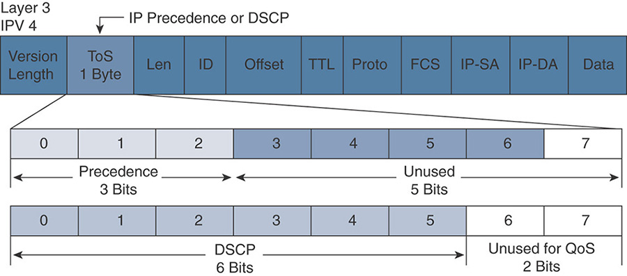
Figure 7-2 DSCP and CoS Fields
Both DSCP and IP Precedence keep the rightmost bit at 0 (this bit is called MBZ, “must be zero”). This means, among other things, that you should never find in a standard network an odd DSCP value. All DSCP values are expected to be even numbers (again, unless the network is nonstandard and the admin uses experimental QoS marking).
DSCP is more complex than IP Precedence because it further divides the 6 left bits into three sections. As a CCIE Wireless, you do not need to be a QoS expert. In fact, you can probably survive the exam with no clear knowledge of DSCP internals, but gaining some awareness will undoubtedly help you design your networks’ QoS policies properly.
Within the DSCP 6-bit label, the three leftmost bits (the 3 MSBs) express the general importance of the traffic, here again on scale from 000 to 111 (0 to 7 in decimal). “Importance” is a relative term. In theory, you could decide that 101 would mean “super important,” while 110 would mean “don’t care.” If you were to do so, you would be using experimental QoS. Experimental, because translating this importance beyond your own network (into the WAN, for example) would become pretty challenging, as any other network could mean anything they wanted with the same bits. To simplify the label structure and help ensure end-to-end compatibility of packet markings between networks, the IETF has worked on multiple RFCs that organize possible traffic types in various categories, and other RFCs that suggest a standardized (that is, common for all) marking for these different categories of traffic. A great RFC to start from is RFC 4594. Reading it will give you a deeper understanding of what types of traffic categories are expected in various types of networks, and what relative importance and marking they should receive. Cisco (and the CCIEW exam) tend to follow the IETF recommendations.
Note
There is in fact only one exception, voice signaling, that the IETF suggests labeling CS5, while Cisco recommends using CS3. The IETF rationale is that signaling belongs to the Voice category and should therefore be right below the audio flows in terms of priority. The Cisco rationale is that this is signaling (statistical exchanges about the voice flow, and not real-time data itself), and that therefore it should come after other types of real-time traffic, such as real-time video.
In most systems, a higher value (for example, 110 vs. 010) represents a type of traffic that is more sensitive to losses or additional delays. This does not mean that the traffic is more important, but simply that delaying or losing packets for that traffic category has more impact on the network user quality of experience. A typical case is real-time voice and FTP. If you drop a voice packet, it typically cannot be re-sent later (the receiving end has only a short window of opportunity to receive this packet on time and play it in the flow of the other received audio packets). By contrast, an FTP packet can be dropped and re-sent without major impact, especially because FTP uses TCP (which will make sure that the lost packet is identified as such and re-sent properly).
Because the three leftmost bits express the general importance of the traffic, and because you have more bits to play with, each set of leftmost bits represent what is called a class of traffic. For example, you could follow the IETF recommendations and label all your real-time video traffic with the leftmost bits 100. But within that category, that class of traffic, you may have different types of flows. For example, your network may carry the business-relevant Spark real-time video traffic and personal traffic (for example, Viber or Facetime). If congestion occurs, and you have no choice but to drop or delay one video packet, which one should you choose? Because you want to keep your job as a network admin, you will probably choose to forward that Spark video packet where your boss is discussing a million-dollar contract and delay or drop that Facetime video packet where your colleague tells his aunt how great her coffee tastes. This wise choice means that you have to further label your video traffic, and this is exactly what the next two bits in DSCP do. They are called drop probability bits. Remember that the last bit on the right is called MBZ (must be zero) and will therefore always be zero in normal networks, and under normal circumstances. Figure 7-3 shows the structure of how DSCP values translate to per-hop behavior (PHB) classes.
The slight complexity of DSCP is that the class bits and the drop probability work in reverse logic.
The three leftmost bits represent the general traffic class, and the convention is that a higher number means a traffic more sensitive to delay and loss (a traffic that you should delay, or drop less, if possible). So you would delay or drop 010 before you delay or drop 100.
By contrast, the drop probability bits represent, within a class, which traffic should be dropped or delayed first. This means that a drop probability of 11 is higher than a drop probability of 10, and the traffic marked 11 will be dropped before the traffic marked 10.
Let’s take a few examples. Suppose that you have a packet marked 101 00 0. Class is 101, drop probability is 00 (and MBZ is, of course, 0).
Suppose that you have a congestion issue and have to delay a packet marked 101 00 0 or a packet marked 100 00 0. Because 101 is higher than 100, you will probably delay 100 00 0. (We suppose here and later that you follow the IETF reasonable and common rules.)
Now suppose that you have to choose between a packet marked 100 10 0 and a packet marked 100 11 0. Because the class is the same, you cannot use the class to make a choice. But because one packet has a drop probability of 11, higher than the other (10), you will choose to delay the packet marked 100 11 0 (because it belongs to the same class as the other but its drop probability is higher). This difference between the class and the drop probability confuses a lot of people, so don’t feel sad if you feel that it is uselessly complicated. In the end, you just get used to it.
Now, if you have to choose between a packet marked 101 11 0 and a packet marked 100 01 0, you will delay or drop the packet marked 100 01 0 because its class is lower than the other one. You see that the class is the first criterion. It is only when the class is the same that you will look at the drop probability. When the class is enough to make a decision, you do not look at the drop probability.
Per Hop Behavior
These DSCP numbers can be difficult to read and remember. Most of the time, the binary value is converted to decimal. For example, 100 01 0 in binary is 34 in decimal. 34 is easier to remember, but it does not show you the binary value that would help you check the class and drop probability values.
The good news is that this general QoS architecture, called Diffserv (for Differentiated Services, because different packets with different marking may receive different levels of service, from “send first” to “delay or drop”), also includes a naming convention for the classes. This naming convention is called the Per Hop Behavior (PHB). The convention works the following way:
When the general priority group (3 bits on the left) is set to 000, the group is called best-effort service; no specific priority is marked.
When the general priority group contains values but the other bits (Drop Probability and MBZ) are all set to 0, the QoS label is in fact contained in 3 bits. As such, it is equivalent to the IP Precedence system mentioned earlier. It is also easily translated into other QoS systems (802.11e or 802.1D) that use only 3 bits for QoS. That specific marking (only 3 bits of QoS) is called a Class Selector (CS), because it represents the class itself, without any drop probability.
When the general priority group ranges from 001 to 100 (001, 010, 011, and 100) and contains a drop probability value, the traffic is said to belong to the Assured Forwarding (AF) class. Transmission will be assured, as long as there is a possibility to transmit.
When the general priority group is set to 101, traffic belongs to the Expedited Forwarding (EF) class. This value is decimal 5, the same as the value used for voice with IP Precedence. In the EF class, for voice traffic, the drop probability bits are set to 11, which gives a resulting tag of 101110, or 46. “EF” and “46” represent the same priority value with DSCP. This is a value you should remember (Voice = 101110 = EF = DSCP 46), but you should also know that 44 is another value found for some other voice traffic, called Voice Admit (but it’s less common). The EF name is usually an equivalent to DSCP 46 (101110). EF is in reality the name of the entire class. Voice Admit (DSCP 44) also belongs to the EF category, but it is handled specially (with Call Admission Control), so you will always see it mentioned with a special note to express that the target traffic is not your regular EF = DSCP 46.
With the exception of EF, all the other classes are usually indicated with a number that shows which level they represent. For example, AF1 will represent all traffic starting with 001. AF4 will represent all traffic starting with 100. Then, when applicable, a second number will show the drop probability. For example, the PHB AF41 represents the DSCP value 100 01 0 (DSCP 34 in decimal).
Table 7-1 summarizes the AF values.
AF Class |
Drop Probability |
DSCP Value |
AF Class 1 |
Low |
001 01 0 |
|
Medium |
001 10 0 |
|
High |
001 11 0 |
AF Class 2 |
Low |
010 01 0 |
|
Medium |
010 10 0 |
|
High |
010 11 0 |
AF Class 3 |
Low |
011 01 0 |
|
Medium |
011 10 0 |
|
High |
011 11 0 |
AF Class 4 |
Low |
100 01 0 |
|
Medium |
100 10 0 |
|
High |
100 11 0 |
When there is no drop probability, the class is called CS and a single number indicates the level. For example, the PHB CS4 represents the DSCP value 100 00 0.
Figure 7-4 will help you visualize the different values. Notice that AF stops at AF4 (there is no AF5, which would overlap with EF anyway, but there is also no AF6 or AF7). Beyond Voice, the upper classes (CS6 and CS7) belong to a category that RFC 4594 (and others) call the Network Control traffic. This is your EIGRP update or your CAPWAP control traffic. You are not expected to have plenty of these, so a common class is enough. Also, you should never have to arbitrate between packets in this class. In short, if you drop your CS6 traffic your network collapses, so you should never have to drop anything there (RFC 4594 sees CS7 as “reserved for future use,” so your network control traffic likely only contains CS6 packets).
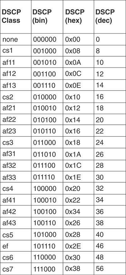
You do not need to learn all the values in this table, but you should at least know DSCP 46 (EF) for Voice, AF 41 (DSCP 34), which are used for most real-time video flows, and CS3 (voice signaling in Cisco networks).
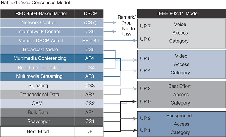
You may wonder how this table maps to the various 12 classes, and this is an important question. Figure 7-5 provides a structured view:
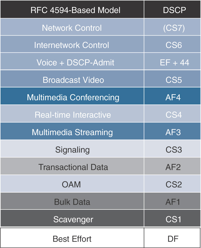
Notice that traffic higher in the list is not “more important.” It is usually more sensitive to delay and loss (as you learned earlier). The reason why this is fundamental to the understanding of QoS is “marking bargaining.” Throughout your QoS career, you will often encounter customers with requirements like this:
Customer: I want to prioritize my business-relevant traffic. I use Spark audio.
You: I see with AVC that you also have Facetime audio traffic. We’ll remark this one as Best Effort and will keep Spark audio as EF.
Customer: Wait, Facetime is not business relevant but it is still Voice, so it is delay sensitive.
You: Yes, but if we mark Facetime EF, it will compete with your business-relevant Spark audio traffic.
Customer: Okay, but can’t you give it something higher than BE that shows that we care for our employees’ personal calls, even if they are not business relevant? Something, like, say 38 or 42?
You: Dear customer, you have absolutely no understanding of QoS.
Your answer to the customer is very reasonable (at least technically). Each class will correspond to specific configuration on switches, routers (and you will see soon, WLCs and APs). Facetime is either in the same bucket as Spark and should be treated the same way (making sure that 50 packets per seconds can be forwarded with low delay, and so on), or it is not business relevant and is sent as best effort (which means “We’ll do our best to forward these packets as fast as we can, unless something more important slows us down”). There is no QoS bargaining, for multiple reasons. One of them is that you probably do not have a QoS configuration for DSCP 42, as your customer suggests. Another reason is that if you create a configuration for DSCP 42, you will have to borrow buffers and queues that are now used for something else, and your Facetime packets will compete with other traffic (for example, with the CEO daily broadcast). If you mark Facetime “something else,” like CS4 or CS5, it will again conflict with other traffic.
These are the reasons why Table 7-1 represents a series of classes, each of which will correspond to a specific set of configured parameters to service that class to best match its requirements and needs. It does not mean that voice is more important than broadcast video, for example. The table just lists typical traffic types and a label that can be applied to each traffic type. In turn, this label will be used on each internetworking device to recognize the associated traffic. With the knowledge of what this traffic type needs, each networking device will forward the packets in conditions that will provide the best possible service, taking into account the current conditions of the network links.
This understanding is also important to realize that Scavenger (CS1) is not “higher” than Best Effort (CS0, 000 00 0), even if it is listed above BE. In fact, all your configurations will purposely send CS1 traffic only if there is nothing else in the queue. If a BE packet comes in, it will go first, and CS1 will only be sent at times when it does not conflict with something else.
IPv6 Layer 3 Marking
DSCP may sound a bit complicated, but it is very efficient. We covered the IPv4 case; now let’s spend a few minutes on IPv6. The good news is that IPv6 QoS marking follows the logic and mechanics of IPv4. The IPv6 header also has an 8-bit field called the Traffic Class field, where you can mark QoS. Just like for IPv4 QoS, we ignore the rightmost 2 bits. They are also called Explicit Congestion Notice bits and are used on some media to inform the other end about a congestion on the line. Because we do not use them in Wi-Fi and because they do not express a QoS category, we ignore them.
The other 6 bits are the same as in the IPv4 header, so you can put your DSCP value there. This makes DSCP easy to use. The same value and categories are expressed in the IPv4 and the IPv6 header, as shown in Figure 7-6.
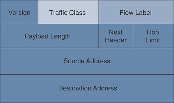
IPv6 adds another section in the header called the Flow Label. This field is not present in IPv4. It is useful for QoS in general because it allows the sender to put a label on a traffic flow. This helps identify all packets in a given flow, and helps classification. With labels, your intermediate networking device can check the label and identify the traffic without having to look at ports or run a deep packet inspection. This is useful in general, but you will not be tested on IPv6 Flow Labels on the CCIE Wireless exam.
Layer 2 802.1 QoS Marking
Remember that Layer 3 QoS marks the global QoS intent for your packet, the general category to which this packet should belong. Your packet is then transported across different media. Each medium has specific characteristics and constraints, and they cannot all categorize QoS families over 6 bits. You saw that DSCP used 6 bits, which translated into (in theory) 64 possible categories. In fact, a count from CS7 to CS0 shows that we are only using 21 values, not 64. However, the DSCP scale is open to 64 possibilities, and your network can decide to implement some experimental values if needed.
Many Layer 2 mediums do not have the possibility of expressing 64 levels of categorization because of physical limitations. Switches, for example, build transmission buffers. You may remember from the section “The Notion of Differentiated Treatment” that the general buffer is split into subbuffers for each type of traffic category. If you had to build 64 subbuffers, each of them would be too small to practically be useful or your general buffer would have to be enormous. In both cases, prioritizing 64 categories over a single line does not make much processing sense when you are expected to switch packets at line rate (1 Gbps or 10 Gbps). However, most switches can use DSCP but they use an 8- or 12-queue model.
The Ethernet world was the first to implement a QoS labeling system. It was built around 3 bits (8 categories, with values ranging from 0 to 7). The initial IP Precedence system at the IP layer was founded on the idea that there would be an equivalence between the Layer 2 and the Layer 3 QoS categories. But as you know, DSCP expanded the model. Today, the Ethernet world is aware that using L3 QoS is reasonable and that Layer 2 should translate the DSCP value, when needed, into the (older) Ethernet 3-bit model. You will find many switches that understand the Ethernet 3-bit QoS model but only use the DSCP value for their traffic classification and prioritization.
You are not taking a Routing and Switching CCIE, so you do not need to be an expert in Layer 2 QoS. However, 802.11 got its inspiration from 802.1 QoS, so it may be useful for you to see the background picture.
That picture may be confusing for non-Switching people, because 802.1 QoS appeared historically in several protocols, and you may have heard of 802.1p, 802.1D, and 802.1Q. In fact, it is just a question of historic perspective. 802.1p is the name of an IEEE task group that designed QoS marking at the MAC layer. Being an 802.1 branch, the target was primarily Ethernet. They worked between 1995 and 1998. The result of their work was published in the 802.1D standard.
Note
In the 802.1 world, lower cases are task groups, like 802.1p, and capital letters are full standards, like 802.1D. This is different from 802.11, where there is only one standard and the standard itself has no added letter. Lower cases are amended to the standard (like 802.11ac), and capital letters indicate deprecated amendments, usually politely named “recommended practices,” like 802.11F.
802.1D incorporates the 802.1p description of MAC Layer QoS but also includes other provisions, like interbridging or Spanning Tree. A revision of 802.1D was published in 2004; however, the 802.1Q standard, first published in 2003 and revised in 2005 and 2011, leverages the 802.1D standard for part of the frame header while adding other parameters (like the VLAN ID). In summary, 802.1p is the original task group, for which results were published in 802.1D and whose elements appear in the 802.1Q section of the 802.1 and 802.3 headers. Very simple.
More critical than history is the resulting QoS marking logic. 802.1p allows for 3 bits to be used to mark QoS, with values ranging from 0 to 7 (8 values total). Each value is called a Class of Service (CoS). They are named as shown in Table 7-2, in 802.1Q-2005.
Table 7-2 Classes of Service Names and Values
Class Name |
Value (Binary/Decimal) |
Best Effort |
0 / 000 |
Background |
1 / 001 |
Excellent Effort |
2 / 010 |
Critical Applications |
3 / 011 |
Video |
4 / 100 |
Voice |
5 / 101 |
Internetwork control |
6 / 110 |
Network Control |
7 / 111 |
Caution
Table 7-2 is not what the original 802.1p-1998 or 802.1D said. We’ll come back to this point soon. However, this is the current practice today, based on 802.1Q.
You see that there is a natural mapping from DSCP CS classes to these 8 values. CS7 and CS6 map to CoS 7 and 6, respectively. Voice (EF) maps to CoS 5, Video (AF4 family) to CoS 4, the critical Signaling (CS3) and Multimedia Streaming (AF3) map to CoS 3, all data (AF2 and CS2) maps to CoS 2, BE is still 0, and Background (CS1) is CoS 1. You need to squeeze several classes into one, and there are a few uncomfortable spots (like CS5), but overall, the DSCP to CoS mapping works.
It would be much more difficult to map the other way around, from CoS to DSCP, because you would not be able to use the 21 values (not to mention 64); you would use only 8. This will come back to us soon.
802.11 QoS Marking
It is now time to look at 802.11 L2 QoS marking. It looks like we took the scenic route to get there, but all you learned will help you make sense of what will look strange in the way 802.11 opposes 802.1 or DSCP. You undoubtedly remember from your CCNA or CCNP studies that the 802.11e amendment, published in 2005 and incorporated in 802.11-2007, lists the labels displayed in Figure 7-7.
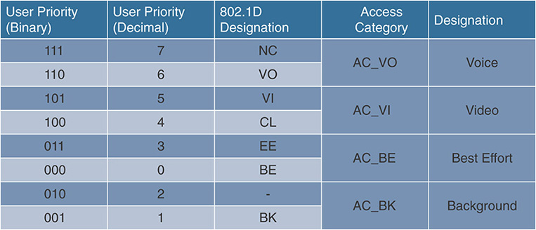
This table is an approximation of the table that appears as 20.i in 802.11e (and Table 10.1 in 802.11-2016). We added the binary value. A few elements are striking, in light of the previous pages:
The labels are called priorities (User Priorities, UP). This is because there is not a lot of buffering play available in a half-duplex medium. We will come back to this point very soon.
UPs are grouped two by two into access categories. Each access category has an intended purpose (voice, and so on).
The values differ notably from the 802.1Q table. This is something a wireless expert must understand.
Table 7-2 was 802.1Q. Table 7-3 is the original 802.1p table that was translated into 802.1D-2004:
Table 7-3 802.1p / 802.1D-2004 Classes
Class Name |
Value (Binary/Decimal) |
Best Effort |
0 / 000 |
Background |
1 / 001 |
Spare |
2 / 010 |
Excellent Effort |
3 / 011 |
Controlled Load |
4 / 100 |
Video |
5 / 101 |
Voice |
6 / 110 |
Network Control |
7 / 111 |
You can immediately see that there is a disconnect between 802.1p/802.1D and 802.1Q-2005. Voice is 6 in 802.1p/802.1d-2004 but 5 in 802.1Q-2005. Similarly, Video gets 5 versus 4, not to mention Excellent Effort downgraded from 4 to 3. At the same time, it looks like 802.11 is following 802.1p/802.1D instead of following 802.1Q. What gives?
It all comes back to this notion of the QoS model. Back at the end of the 1990s, when the 802.1p group was working, a standard model was around four queues, and a new trend was to add more queues. The most urgent traffic was seen as Network Control, and the most urgent client data traffic was seen as Voice. This is what gave birth to the 802.1p model.
When the 802.11e work started in 2000, it built on the work of a consortium, Wireless Multimedia Extensions (WME), led by Microsoft, that was already trying to implement QoS markings among Wi-Fi vendors. They (of course) followed the IEEE recommended values of the days (802.1p). The 802.11e draft was finished in 2003, and the 2003 to 2005 period was about finalizing details and publishing the document.
In between, the IETF recognized that Network Control Traffic should be split into two categories: level 6, which is the standard internetwork control traffic, and an additional category of even higher level that should in fact be reserved for future use or for emergencies (label 7). In such a model, Voice is not 6 anymore but 5, and Video moves from 5 to 4. This change was brought into the inclusion of 802.1D into the revised 802.1Q-2005, but 802.11e was already finalized.
The result is a discrepancy between the standard 802.1Q marking for Voice and Video (5 and 4, respectively), and the standard 802.11e marking for these same traffic types (6 and 5, respectively). A common question you will face as an expert is: Why did 802.11 keep this old marking? Why did they not update like 802.1Q did?
There are multiple answers to this question, but one key factor to keep in mind is that the 802.11e marking is neither old, wrong, obsolete, nor anything along that line. Ethernet is a general medium that can be found at the Access, Distribution, and Core layers. You expect any type of traffic on such a medium, including routing updates. By contrast, Wi-Fi is commonly an access medium. You do not expect EIGRP route updates to commonly fly between a wireless access point and a wireless client (wireless backbones are different and are not access mediums). As such, there is no reason to include an Internetwork Control category for 802.11 QoS. We already lose UP 7 if we keep it for future use as recommended by IETF; it would be a waste to also lose UP 6 and be left with only 5 values (plus 0). Therefore, the choice made by the IEEE 802.11 group, to keep the initial 802.1D map, is perfectly logical, and is not laziness (and yes, the 802.11 folks also know that 802.1Q changed the queues). In the future, it may happen more that 802.11 becomes a transition medium toward other networks (for example, toward your ZigBee network of smart home devices). If this happens, it may make sense to change the 802.11e queues to include an additional Internetwork Control queue. Until that day comes, a simple translation mechanism happens at the boundary between the 802.11 and the 802.1 medium (UP 6 is changed to CoS 5, UP 5 to CoS 4, while the rest of the header is converted too). As a CCIE Wireless, you need to know that these are the right markings and resist the calls to unify the markings. Current best practices are to use UP6/PHB EF/DSCP 46/CoS 5 for Voice and UP 5/PHB AF41/DSCP 34/CoS 4 for real-time video. The only exception is that CoS tends to be ignored more and more, as DSCP is used instead (more on this in the upcoming section). Any request to use UP 5 for Voice is a trap into which you should not fall.
DSCP to UP and UP to DSCP Marking
In most scenarios, you should try to use DSCP to express your QoS intent (because DSCP is independent from the local medium). However, there are cases where you need to work from UP and decide the best DSCP, or when you need to decide which UP is best for a given DSCP value. These requirements mean that you need to know what the recommended practices are for this mapping. Fear not, there is a macro that we will examine in the “Configurations” section that will help you configure the right numbers.
Downstream
Downstream traffic will come from the wire and will have a DSCP value. You need to decide which UP to use. Table 7-4 shows the Cisco recommended mapping for a 12-class QoS model. You will see each of 12 categories, their associated recommended DSCP marking (as per RFC 4594), and the associated recommended UP marking. This mapping, shown in Figure 7-8, is not just recommended by Cisco but is also an IETF standard (RFC 8325, https://tools.ietf.org/html/rfc8325).
Table 7-4 UP to DSCP Recommended Mapping
Incoming UP Value |
Recommended DSCP Value to Map To |
0 - 000 |
0 (CS0) – 000 00 0 |
1 - 001 |
8 (CS1) – 001 00 0 |
2 - 010 |
16 (CS2) – 010 00 0 |
3 - 011 |
24 (CS3) – 011 00 0 |
4 - 100 |
32 (CS4) – 100 00 0 |
5 - 101 |
34 (AF41) – 100 01 0 |
6 - 110 |
46 (EF) – 101 11 0 |
7 - 111 |
56 (CS7) – 111 00 0 |
Notice that this model uses all UPs (except 7, still reserved “for future use”). This rich mapping implies that some traffic, within the same access category (AC), will have different UPs. You will see in the “Congestion Management” section that the access method (AIFSN, TXOP) is defined on a per access category basis. This implies that both UPs in the same AC should have the same priority level over the air. However, Cisco APs (and most professional devices) have an internal buffering system that prioritizes higher UPs. In other words, although there is no difference between UP 4 and UP 5 as far as serialization goes (the action of effectively sending the frame to the air), the internal buffering mechanisms in Cisco APs will process the UP 5 frame in the buffer before the UP 4 frame, thus providing an internal QoS advantage to UP 5 over UP 4, even if you do not see this advantage in the IEEE 802.11 numbers.
Upstream
Upstream traffic should come with DSCP marking (see the next section). In that case, you should use DSCP and ignore UP. However, you may have networks and cases where UP is all you have to work from, and you need to derive the DSCP value from the UP value. This is a very limiting case because you have only 8 UP values to work from, and this does not fit a 12-class model. It also makes it impossible to map to potentially 64 DSCP values. Even if you keep in mind that only 21 DSCP values are really used (counting all the AF, CS, and EF values in the DSCP table in the previous pages), 8 UPs definitely is not enough. So you should avoid using UP to derive DSCP whenever possible, but if you have to make this mapping, the recommended structure is shown in Table 7-4.
Note that the mapping structure is very basic: For most UP values, simply map to the generic Class Selector (CS). Then, map Video and Voice to their recommended DSCP value (AF41 and EF, respectively).
Note
There is an important semantic exception to make for this table. You will see that UP 7 is recommended to be mapped to CS 7. This is the mapping recommendation. This mapping recommendation does not mean that you should have UP 7 or CS7 traffic in your network. It just says that if you have UP 7 traffic in your network, the only logical DSCP value to which UP 7 could be mapped is CS 7.
However, you should not have any UP 7 (or DSCP CS 7) traffic in your network, first because there is typically no network control traffic that would flow through your Wi-Fi access network (unless your Wi-Fi link bridges to other networks, in which case it is not “access” anymore but has become “infrastructure”), but also because CS7 is reserved for future use. So the actual recommendation is to remap any incoming CS 7 traffic (or UP 7 traffic) to 0, because such marking is not normal and would be the sign of something strange happening in your network (unless you are consciously using this marking for some experimental purpose). You will see in the “Configurations” section how this remarking is done.
Even if you have network control traffic flowing through your Wi-Fi network, the IETF recommendation is in fact to use CS 6 and map it to UP 6. It will be in the same queue as your voice traffic, which is not great. But UP 6 is better than UP 7 (which should stay reserved for future use). The expectation is that you should not have a large volume of network control traffic anyway. Therefore, positioning that traffic in the same queue as voice is acceptable because of the criticality of such traffic and the expected low volume. If you have a large volume of network control traffic over your Wi-Fi link, and you plan to also send real-time voice traffic on that link, you have a basic design issue. A given link should not be heavily used for voice traffic and be at the same time a network control exchange highway.
Trust Boundary and Congestion Mechanisms
Marking packets correctly is critical, and understanding how to translate one marking system into another when packets are routed or switched between mediums is necessary. However, marking only expresses the sensitivity of a packet to delay, jitter, loss, and bandwidth constraints. After this sensitivity is expressed, you need to look at it and do something with it.
Trust Boundary
At this point, you should understand that traffic can be identified (using various techniques, including Deep Packet Inspection, or simple IP and port identification). After identification is performed, you can apply a label to that traffic to express its category. This label can be applied at Layer 2, at Layer 3, or both. Layer 3 expresses the general intent of the traffic, while Layer 2 expresses the local translation of that general intent. After a packet is labeled, you do not need to perform classification again (you already know the traffic category)—that is, if you can trust that label. This brings the notion of trust boundary. The trust boundary represents the point where you start trusting the QoS label on a frame or packet. At that point, you examine each packet and decide its classification and associated marking. Beyond that point, you know that packets have been inspected and that their marking truly reflects their classification. Therefore, all you have to do is act upon the packet QoS label (to prioritize, delay, or drop packets based on various requirements examined in the next section).
But where should the trust boundary be located? Suppose that you receive a packet from a wireless client and this packet is marked EF (DSCP 46). Should you automatically assume that this packet carries voice traffic and should be prioritized accordingly, or should you examine the packet with Deep Packet Inspection (DPI) and confirm what type of traffic is carried? You may then discover that the packet is effectively voice, or that it is BitTorrent.
There is no right and wrong answer for this trust question, and Figure 7-9 illustrates the various options. In a corporate environment, where you expect only corporate devices and corporate activity, you may decide to fully trust your endpoints and clients. From an efficiency standpoint, this scenario is optimal because you should classify and recognize traffic as close as possible to the traffic source. If classification is done at the endpoint level, and all you have to do is act upon the marking displayed in the endpoint packets, your network QoS tasks are all around prioritization and congestion management. Classifying at the endpoint level removes the need for the network to perform DPI. DPI is CPU-intensive, so there is a great advantage in trusting the client marking. In that case, your trust boundary is right at the client level (points labeled 1 on the left).
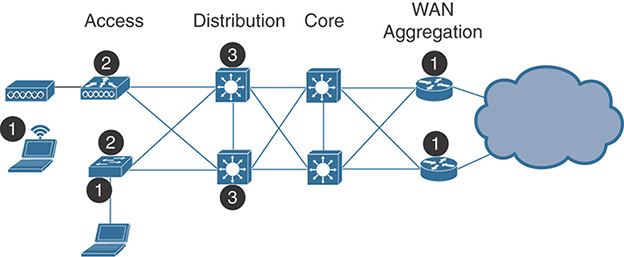
However, in most networks, you cannot trust the client marking. This lack of trust in the client QoS marking is not necessarily a lack of trust in the users (although this component is definitely present in networks open to the general public) but is often a consequence of differences in QoS implementations among platforms (in other words, your Windows clients will not mark a given application the same way as your MacOS, iOS, or Android clients). Therefore, you either have to document each operating system behavior for each application and create individual mappings and trust rules accordingly, or run DPI at the access layer (on the access switch for wired clients and on the AP or the WLC for wireless clients). In that case, your trust boundary moves from the client location to the access layer. This location of the trust boundary is also acceptable. This is the reason why you will see NBAR2/AVC be configured commonly on supporting access switches, and on APs/WLCs. They are the access layer (labeled 2 in the illustration). On the other side of the network, the first incoming router is the location where AVC rules will also be configured, because the router is the incoming location for external traffic. (It is the point under your control that is located as close as possible to the traffic source when traffic comes from the outside of your network, and is therefore also labeled 1 in the illustration.)
If you cannot perform packet classification at the access layer, you can use the aggregation layer (labeled 3 in the illustration). However, traffic from all your access network transits through aggregation. Therefore, performing classification at this point is likely to be highly CPU intensive and should therefore be avoided, if possible, especially if classification means DPI.
One point where you should never perform classification is at the core layer. At this layer, all you want to do is to switch packets as fast as possible from one location to another. This is not the place where traffic inspection should happen.
As a wireless expert, you should know that the point of entry to your network (the WAN aggregation router) is one location where classification should occur. You should also decide whether you can trust your wireless clients’ marking. As you will see later in this chapter, in most cases you cannot trust the client marking. The reason is not so much that you cannot trust your users but rather that different operating systems have different rules for application QoS marking. Therefore, unless your network is exclusively composed of iOS and MacOS devices, with a very small set of applications, running AVC on the WLC will be required if you want to have precise QoS rules in your network. This is a common rule in the CCIE Wireless exam. In the real world, running AVC consumes CPU resources, and you will want to examine the impact of AVC on your WLCs CPU before freezing your configuration to AVC Enabled and leaving for a 3-month vacation.
Congestion Management
The trust boundary determines the location where you start trusting that the QoS label present on a packet truly reflects the packet classification. Regardless of where the trust boundary lies, there will be locations in the network (before or after the trust boundary) where you will have to act upon packets to limit the effect of congestion. It is better if your trust boundary is before that congestion location (otherwise you will act upon packets based on their QoS label without being sure that the QoS label is really representing the packet class).
Multiple techniques are available to address existing or potential congestion. In QoS books, you will see many sections on this topic because this is one of the main objectives of QoS. However, as a wireless expert, you do not need deep insight into switching and routing techniques to address observed or potential congestion. In the context of CCIE Wireless, this section is limited to the techniques that are relevant to your field.
802.11 Congestion Avoidance
One key method to limit the effect of congestion is to avoid congestion in the first place. This avoidance action is grouped under the general name of congestion avoidance.
In your CCNA studies, you heard about the 802.11 access method, Carrier Sense Multiple Access with Collision Avoidance (CSMA/CA). This is one implementation of congestion avoidance, where any 802.11 transmitter listens to the medium until the medium is free for the duration of a Distributed Interframe Space (DIFS).
Note
Remember that there are two time units in a cell, the slot time and the short interframe space (SIFS). With 802.11g/a/n/ac, the slot time is 9 μs and the SIFS 16 μs. The DIFS is calculated as 1 DIFS = 1 SIFS + 2 slot times. The slot time is the speed at which stations count time (especially during countdown operations).
This “wait and listen” behavior is already a form of congestion avoidance. Then, to avoid the case where more than one station is waiting to transmit (in which case both stations would wait for a silent DIFS, then transmit at the end of the silent DISF, and thus collide), each station picks up a random number within a range, then counts down from that number (at the speed of one number per slot time) before transmitting. At each point of the countdown, each station is listening to the medium. If another station is transmitting, the countdown stops, and resumes only after the medium has been idle for a DIFS. This random number pick, followed by countdown, is also a form of congestion avoidance because it spreads the transmissions over a period of time (thus limiting the number of occurrences where two stations access the medium at the same time).
If your network is 802.11n or 802.11ac, it must implement WMM, which is a Wi-Fi Alliance certification that validates a partial implementation of 802.11e. WMM validates that devices implement access categories (AC). It tests that a device has four ACs but does not mandate a specific DSCP to UP mapping, and within each AC does not verify which of the two possible UPs is used. As 802.11n was published in 2009, it is likely that your networks will implement the WMM access method rather than the legacy access method.
WMM also implements the part of 802.11e called Enhanced Distributed Channel Access (EDCA). With WMM and EDCA, your application classifies traffic into one of the four ACs, and the corresponding traffic is sent down the network stack with this categorization. In reality, this classification can be done through a socket call at the application layer that will either directly specify the AC or, more commonly, will specify another QoS value (typically DSCP, but sometimes UP), that will in turn be translated at the Wi-Fi driver level into the corresponding AC.
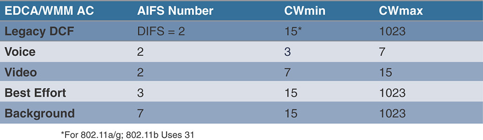
Each AC has a different initial wait time (the DIFS for non-WMM traffic). Because that initial duration is arbitrated depending on which AC the traffic belongs to, the initial wait time is called the Arbitrated Interframe Space (AIFS). Because it is calculated in reference to the DIFS, it is also often called the Arbitrated Interframe Space Number (AIFSN). The AIFSN is smaller for ACs intended for traffic that is more sensitive to loss and delay. This difference means that the driver will start counting down sooner for voice traffic than, for example, best effort or background traffic.
For each packet, the driver also picks up a random number. After the medium has been idle for the duration of the AIFSN matching the AC within which the packet is waiting, the driver will count down from that random number. The range of numbers from where the random number is picked is called the Contention Window (CW). You will see CW as a number, but keep in mind that a random number is picked within a range. So if you see CW = 15, do not think that the device should wait 15 slot times. A random number will be picked within 0 and 15, and the device would count down from that number.
The same logic applies here as for the AIFSN. ACs more sensitive to loss and delay will pick a number within a smaller range. Although the number is random (and therefore any of the ACs may pick, for example, 1 or 2), ACs with a small range have more statistical chances of picking smaller numbers more often than ACs with larger ranges.
When the countdown ends (at 0), the matching packet is sent. All four ACs are counting down in parallel. This means that it may (and does) happen that two ACs get to 0 at the same time. This is a virtual collision. 802.11 states that, in that case, the driver should consider that a collision really occurred and should apply the collision rules (below). However, some vendors implement a virtual bypass and send the packet with the highest AC, and either only reset the counter of the packet with the lower AC or send that packet with the lower AC right after the packet with the higher AC. It is difficult to know whether your client vendor implements these shortcuts unless you have visibility into the driver. Cisco does not implement these shortcuts because they violate the rules of 802.11, and because they result in weird imbalances between applications. However, Cisco implements 8 queues (per client), which means that packets with UP 5 and packets with UP 4, although belonging to the same AC, will be counting down in parallel (whereas a simpler driver would count down for one, then count down for the other, because the packet would be one after the other in the same queue). When two packets of the same AC but with different UPs end up at 0 at the same time, this is the only case where the packet with larger UP is sent first, then (after the matching AIFSN) the packet with the lower UP is also sent. This allows for a differentiated treatment between packets of the same AC but different UPs while not violating the 802.11 rules (that treats inter-AC collisions as virtual collisions, not intra-AC collisions).
Collisions can occur virtually, but also physically (when two stations send at the same time). In this case, a collision will be detected for unicast frames because no acknowledgement is received (but note that a collision will not be detected by the sender of broadcast or multicast traffic). In that case, the contention window doubles. Most drivers double the random number they picked initially, although 802.11 states that the window itself should double, and a random number can be picked from this new, twice-as-large, window. The reason for doubling the number itself is another form of congestion avoidance. If a collision happened, too many stations had too much traffic to send within too short a time interval. Because you cannot reduce the number of transmitters (you have no control over the number of stations having traffic to send at this point in time), your only solution is to work on the time dimension and extend the time interval across which that same number of stations is going to send.
This doubling of time is logical from a protocol design standpoint but not very efficient for time-sensitive traffic. Therefore, an upper limit is also put on this extension of the contention window. The contention window can only grow up to a maximum value that is smaller for voice than for video, smaller for video than for best effort, and smaller for best effort than for background traffic. Therefore, the contention window can span between an initial value, called the minimum contention window value (CWmin), and a max number, called the maximum contention window value (CWmax).
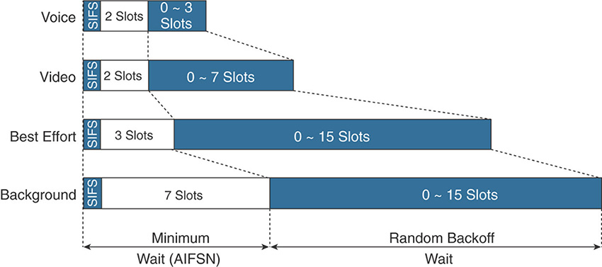
The different AIFSN and CW values are represented in Figure 7-10. You will note that the AIFSN for voice has the same value as the DIFS. However, the CWmin provides enough statistical advantage to voice that a smaller AIFSN would not have been useful. As a matter of fact, early experiments (while 802.11e was designed) showed that any smaller AIFSN for voice or video would give such a dramatic advantage to these queues over non-WMM traffic that non-WMM stations would almost never have a chance to access the medium.
Also, it is the combined effect of the AIFS and the CW that provides a statistical differentiation for each queue. As illustrated in Figure 7-11, you can see that voice has an obvious advantage over best effort. Non-WMM traffic would have the same AIFS/DIFS as the voice queue, but the CW is so much larger for best effort that voice gets access to the medium much more often than best effort.
Note that if you capture traffic and look at the CW values, you may not see the right numbers. This is because 802.11 defines them as exponents, as shown in Figure 7-12.
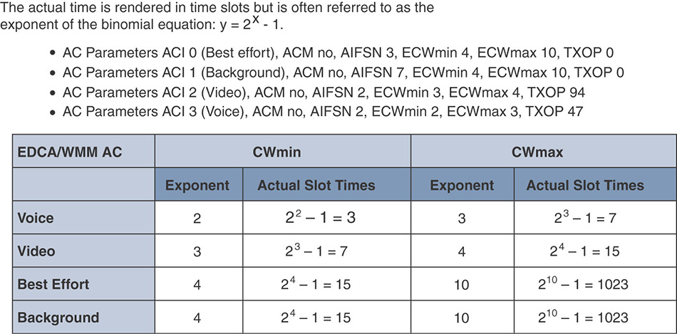
A value of 3 (0011) would in fact mean (23 − 1), which is 7. This exponent view provides a compact way to express numbers with the least number of consumed bits.
TXOP
Another technique to avoid congestion is to regulate the access to the medium. Wi-Fi is particular in its medium access logic, where each packet requires an individual contention with its associated random backoff timer. This logic is reasonably well adapted for data packets but can be detrimental for real-time packets because the time counter does not get reset between packets. Let’s take a worst-case scenario and suppose that your voice application samples audio every 10 milliseconds. We saw before that the wireless card does not need 10 milliseconds to send 10 milliseconds worth of audio, which translates to a few hundred bytes at most. However, keep in mind that each voice packet carries a timestamp in its RTP header. Suppose that you have two audio frames in your buffer. You send the first one, and at the end of the transmission the medium is still free. Yet, you need to wait for a DIFS (or an AIFS), then count down from a random backoff number before sending the next frame. Bad luck, the cell is congested, and other stations send before you get down to 0. If you look back at Figure 7-10, you will see that voice and video have the same AIFS. You will also see that voice can pick up to three slots for its backoff timer. By contrast, best effort AIFS is 3 slots long, and the random backoff is picked in a contention window ranging from 0 to 15 slots. This means that your voice packet may very well compete against a video or best effort packet, or both, and lose both races (if these packets picked a low random backoff timer).
You may think that this is not a big issue because your countdown will resume (not restart), and you will get to 0 eventually; you are right, at least on paper. One difficulty is that the original 802.11 said how long you should wait but did not say how long your transmission should be. 802.11 defined only a max MTU (an 802.11 frame is max 12,246 bits long, with the MAC and PHY headers). If your competing stations sent that max MTU at 6 Mbps, the transmission time is about 2 milliseconds.
Note
You can play with transmission numbers using this tool: https://sarwiki.informatik.hu-berlin.de/Packet_transmission_time_in_802.11.
If your phone operates in the 2.4 GHz band (remember, 802.11e was designed in 2005), you may compete against a 1 Mbps transmission, and this would represent more than 12 milliseconds of airtime. If your voice packet picked three slots, you may lose the race against three video frames, or one video frame and one best effort frame. Suppose that, in this partly congested environment, you also collide once or twice. You see that you may soon face a scenario where voice packets start piling up in your stack. Yet, if we could let you send a few more voice frames in sequence, you could catch up on this increasing delay without impacting the other transmissions too much, especially because voice packets are very small (that is, they do not consume a lot of airtime, even at low data rates). At the scale of your voice call, 30 milliseconds make a difference. At the scale of an FTP transmission, 30 milliseconds are irrelevant.
Because 802.11 could not control the max transmission time of a single frame, the 802.11e group decided to control the overall transmission time of several frames by also playing with the real-time nature of the voice and video queue. So 802.11e creates the notion of Transmit Opportunity (TXOP). In each beacon, the AP advertises TXOP values for each of the four ACs. Each TXOP is a duration, in units of 32 microseconds. Without TXOP, each station can send only one frame at a time. With TXOP, each station can transmit one frame, then continue transmitting in a burst as long as the transmission is smaller than the TXOP for that queue.
Figure 7-13 shows the 802.11e TXOP values for all ACs.
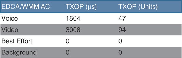
Those values mean that, if you are transmitting traffic from the voice AC, after you gain access to the medium with the AIFS/Random backoff mechanism, you can keep transmitting for up to 1504 microseconds. Because each voice packet is small, this maximizes your chances of emptying your buffer. If you are transmitting a video flow, you can transmit even longer, up to 3 milliseconds. This is because video packets are typically much larger than voice packets, so you will need more time to empty your buffer. However, you should not use so much time that you would starve voice transmitters, and this is why the ratio 1 to 2 (video gets twice as long a TXOP as voice) was designed.
Best effort and background get 0 TXOP. This means that these ACs cannot extend beyond the regular transmission mechanisms. In other words, no transmission burst for these ACs. Each frame has to go through the individual countdown, without the possibility of bursting after medium access is granted. Also, keep in mind that each queue is addressed individually. So you cannot, for instance, send one best effort queue and then continue with a burst of voice packets. Countdown and medium access are parallel (independent) for each queue buffer. If you get access to the medium at the end of a best effort packet countdown, this is the packet you send; while your voice or video queues are virtually contending with this best effort packet, each AC is counting down in parallel, individually.
This TXOP mechanism, implemented as part of the original 802.11e in 2005 and the corresponding Wi-Fi Alliance WMM certification, saved a lot of time for the voice and video ACs, at least until 802.11n and then 802.11ac came into play. These two amendments allow a new form of transmission: the block. In fact, block transmissions were described in 802.11e, but their acknowledgement mechanism (each frame in the block must be acknowledged individually) made them somewhat impractical. 802.11n and 802.11ac allow a transmitter and a receiver to agree on a block transmission and acknowledge individual components of the block in a coded single ACK message. This efficiency allowed 802.11n and 802.11ac transmitters to use blocks extensively. Why are we mentioning this? Because a block is technically a single frame. With a max block size of more than 65,535 bytes for 802.11n and 4,692,480 bytes for 802.11ac, the maximum transmission duration of a single block can reach 5.484 ms. This is a major problem. With WMM, your AP announces TXOPs in its beacons and states that the voice queue can send at most 1.5 ms worth of data, video at most 3 milliseconds worth of data, and best effort and background as long as they want, as long as it is a single frame each time. If it is a block, that “single frame” gets up to 5.5 ms worth of airtime, much better than voice or video. So, in short, blocks create a disadvantage for your high-priority queues.
The 802.11 working group realized this issue and modified the TXOP values in the revised version of the 802.11 standard published in 2016, as displayed in Figure 7-14.
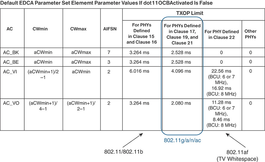
From this table, you can see that two major changes were made:
Now each AC has its own TXOP. This allows the AP to provide limits to all queues, regardless of whether a station is using blocks. BE and BK TXOPs values are close to those of voice, because tests showed that this approximate equality was enough to provide a statistical advantage to voice without starving the BE or BK queues. Video has a longer TXOP because it is both real-time and bursty.
The TXOP limits are different depending on the protocol you use (802.11e had a single set of TXOP, regardless of what protocols you would enable in your cell). 802.11b is much slower than 802.11g/a/n/ac, so it makes sense to have larger values for this protocol to give more time to the voice or video queue to empty their buffer within each TXOP. 802.11af sets “0” for BE and BK because this TV whitespace protocol does not use blocks.
This revision of the TXOPs is much more efficient than the previous 802.11e TXOP system. In fact, the old system is considered as a source of performance issues in any cell where voice traffic is mixed with data traffic and stations that use blocks. In a Cisco WLC, as we will see in the “Configurations” section, this revision of the TXOP values is called Fastlane, and you should always use them. The values in the table above are expressed in milliseconds. A detail on the 802.11g/a/n/ac values, with both the values in milliseconds and the values in 32 microsecond slots, is shown in Figure 7-15.
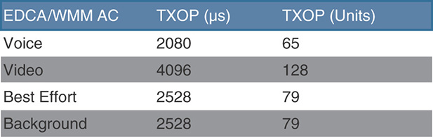
CAC
TXOP is a way to provide more transmit opportunities to selected traffic categories, but also to control and limit the amount of consecutive transmissions. 802.11e also implemented another technique, directly derived from Unified Communications: Call Admission Control (CAC).
Caution
CAC is used in the Unified Communication (UC) world and the Wi-Fi world, but they are very different features. UC CAC is typically implemented on a voice control server (like Cisco Unified Communications Manager, CUCM) and tests end-to-end bandwidth and links performance. Based on these measurements, the voice control server would allow or disallow specific calls. For example, the server would block (busy tone) your call to number 1234 if it found that the end-to-end link to the phone serving this number does not provide enough performances to allow a workable call. But the server could allow your call to 4422 if it found that the end-to-end link to the phone serving this number does provide enough performances to allow a workable call. Therefore, allowing or disallowing calls is based on partial or end-to-end link analysis on a per-call basis.
By contrast, the CAC implemented in Wi-Fi is solely about the RF link and is not related to any voice control server. Wireless CAC is managed only by the Wi-Fi infrastructure, independently of the rest of the infrastructure. You will in fact encounter two names for this feature: Wireless CAC and ACM (Admission Control Mandatory). ACM is the term used in 802.11 and WMM. Wireless CAC is the common name used among many vendors.
The principle of ACM is to restrict access to target ACs, specifically the voice or video AC. When ACM is enabled for an SSID, ACM = 1 is advertised in the AP beacons and probe responses for the matching AC. An example is provided in Figure 7-16.
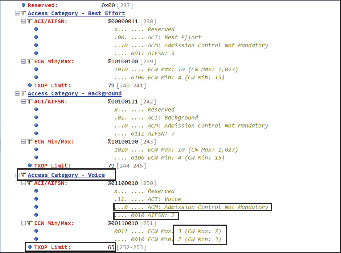
802.11e states, and the WMM certification verifies, that a station should not send traffic in the voice AC when ACM is enabled, without initially requesting service. This service request takes the form of an Add Traffic Stream Request (ADDTS) sent by the client side. In this action frame, the station describes the candidate’s traffic intended to be exchanged in the restricted AC. This description is done in two fields: Traffic Specification (TSPEC), a mandatory field, and Traffic Class (TCLAS), another, but optional, field.
Note
For this section, just like for the others, we only focus on 802.11e EDCA, the part of 802.11e that describes distributed access function to the cell and that is implemented by vendors today. 802.11e also describes a coordination function where the AP takes over the cell and distributes the right to send (HCCA, Hybrid Coordinated Function Controlled Channel Access), but this mode is not implemented widely (if at all), not implemented by Cisco, not tested by the Wi-Fi Alliance, and therefore nonessential for your expertise in the real world and on the CCIE Wireless exam.
TSPEC describes what the intended traffic would look like and is the most important field for this ADDTS exchange. You will find more details on this field in 802.11-2016 section 9.4.2.30. The key elements of the TSPEC field are displayed in Figure 7-17.
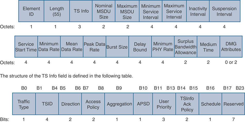
You do not need to know these fields by heart, but it is useful to understand them, to determine why some stations support TSPEC whereas most others do not. TSPEC provides information about the traffic, not only in terms of target UP but also in terms of minimum and maximum expected frame sizes for this traffic, including possible bursts, possible silences between frames, the minimum and maximum data rates needed to make the flow sustainable, and the airtime consumption for the flow. Deep knowledge of both 802.11 and the traffic flow (codec) are needed to provide information in the TSPEC field. This is the main reason why TSPEC support is common for hard phones (for example, Cisco 8821 or 7926) but very uncommon for software applications on smartphones. In this last case, app developers typically understand the software part (codec and so on) but have no idea about Wi-Fi, and would have no clue on the max MSDU or the aggregation support, because these parameters not only require Wi-Fi expertise (that they typically lack) but also depend on the Wi-Fi driver characteristics. App developers have no information about the possible platforms of Wi-Fi drivers. On their side, Wi-Fi driver developers have no information about all the possible real-time apps that will be running on the smartphone. Such coordination between these two unrelated and disconnected worlds is very difficult, and TSPEC is therefore very uncommon on smartphones.
Note
Please note that there are some exceptions; for example, when the real-time application is developed by the smartphone manufacturer, or when the smartphone gets “specialized” (that is, optimized for a specific application). An example is Vocera, a voice company making badges primarily for the healthcare market. Vocera developed a specific version of a Motorola smartphone in which the driver was optimized for the Vocera application. This smartphone supports TSPEC. Such examples are uncommon.
The ADDTS request can also include an optional field called the Traffic Class (TCLAS). This field includes the target AC, and also a Traffic Classifier (TC) field. TC is intended to provide more information about the flow upper layers, such as Layer 3 source and destination addresses (IPv4 or IPv6), Layer 4 ports and protocol, VLAN details, and so on. In most cases, this information is not relevant to the AP and is available in the payload part of the frame anyway, so the TCLAS element is optional and often skipped.
The AP receives the ADDTS request and examines the TSPEC field. Based on the traffic description, the AP estimates whether there is enough bandwidth available to add the requested flow to the cell. The determination method is proprietary. In Cisco WLCs, you can configure the bandwidth limit for this determination. Some solutions also look at the traffic description to figure out whether the described pattern matches the expectations of such a traffic class. For example, an ADDTS for AC_VO that describes large bursty frames would look suspicious, especially if the payload indicates a well-known BitTorrent port. Such a flow might be declined regardless of the available bandwidth.
After the AP has made the determination of whether to accept or decline the traffic, it will return an ADDTS response to the client that includes the decision (accept or reject). If the decision is to accept, then the client can start sending the flow (the ADDTS response includes a validity period during which the flow should start). If the decision is reject, the station cannot use that AC at that time for that flow. The station can ask again (with the same or different codec), ask for another AC, or revert to sending the traffic directly into an AC that does not have ACM enabled. Most hard phones would display a Network Busy message on the screen when this rejection happens. (It is a visual Network Busy sign, not an audio sign, as this rejection has nothing to do with the audio/Unified Communications part of your phone.) In most cases you would try again, which would trigger a new ADDTS request from your phone (with the hope that the network has more space for your call as you retry).
In all cases, the station cannot send into the target AC, if ACM is enabled, without going through the ADDTS request first, and it cannot send into that AC if the AP responds with a reject. The Wi-Fi Alliance validates this behavior through the WMM certification. This means that any WMM certified device would obey these rules. Because the WMM certification is mandatory to obtain the Wi-Fi-n or Wi-Fi-ac certification, you can be confident that any 802.11n/ac device would obey these rules.
BW Contracts
A last way to control congestion in Wi-Fi networks lies in bandwidth contracts. This is your standard bandwidth limitation logic. In the wired world, you find two forms of this bandwidth control, called policing and shaping, as shown in Figure 7-18.
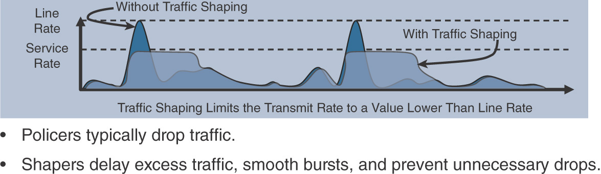
Policing admits traffic up to a configured bandwidth and deletes the rest. In the figure, any traffic above the service rate would be deleted. Shaping defines notions of buckets, where you can store that excess traffic temporarily, then send it over time. In other words, shaping also limits the bandwidth and delays the excess traffic to send it over a longer period of time. However, if the temporary storage bucket gets full, the extra traffic will be deleted.
Wi-Fi also offers such options. You can control the bandwidth with a maximum traffic rate to which you can also add a burst rate. This burst rate determines how much more than the target bandwidth you will accept in your buffer. This additional traffic will be stored temporarily and sent over time. However, even if the system displays values in kilobits per second, for example, you should not expect the Wi-Fi scheduler to act like a switch scheduler. In a Catalyst 6500, for example, transmissions over a link can be evaluated every 0.25 milliseconds. This means that the consumed bandwidth, along with the additional incoming traffic (your burst), can be compared 4,000 times per second. As a result, the throughput impression, when seen from the outside, may appear very linear and close to the configured intended rate.
Note
The fact that the rate is calculated every 0.25 ms should not obfuscate the limited lengths of the queues and buffers. If you get more data than the queue can hold, recalculating the throughput at the next 0.25 ms interval will not prevent some packets from being removed because they did not fit in the buffer, thus resulting in the loss issue described at the beginning of this chapter.
Such recalculation is not so frequent in an access point for several reasons:
The AP must face the fact that some transmissions will fail (ACK not received); the retransmission should not be considered as additional consumed bandwidth but as the realization of the same bandwidth intent. Therefore, a software process is needed to deduce the retries from the effective bandwidth consumption. This need is much more uncommon on an Ethernet link.
The AP must face the fact that your rate will change (different MCS at different locations) and that random silences (backoff timers) are disrupting the transmission rate. By contrast, Ethernet links use a fixed rate (for example, 1 Gbps), and transmission always occurs at that line rate and typically in a full duplex mode. This difference means that the AP needs a software function to calculate the effective consumed bandwidth based on the amount and sizes of packets transmitted over a sampled period of time.
As a result, and although you will configure bandwidth limitations (called Bandwidth Contracts in Cisco WLCs) in kbps, you should be aware that this bandwidth is an average over time, not a precise limit at milliseconds scales.
Bandwidth contracts are very popular in Wi-Fi circles. They come from the times when WLANs (typically guest networks) were shared with contractors, and there was a need to ensure that these contractors would not abuse that available (and “free”) bandwidth. Bandwidth contracts started as downstream constructs only, but then the pressure from multiple types of customers (often with limited understanding of Wi-Fi and QoS) brought the need to allow for upstream bandwidth control as well. Then, the multiplicity of implementations and scenarios brought the configuration of these contracts in multiple areas of the AP or WLC interfaces. As we’ll see in the “Configurations” section, you can configure BW limitations in QoS profiles, WLANs, and device profiles, and you can override each of those with AAA VSAs. You can also configure different limitations for TCP and UDP traffic, each with intended limitations and accepted bursts (shaping logic).
In a different implementation, bandwidth control can be enabled with a feature called Airtime Fairness (ATF). ATF is very different from bandwidth contracts because it has the possible support of flexible boundaries, as you will see later in this section.
Despite the popularity of Wi-Fi bandwidth contracts, the expert in you should carefully weigh the benefits from such strategies. Bandwidth contracts are solid boundaries (although they are not calculated in real time, so they are somewhat bursty). A direct objective is to prevent some traffic from consuming all available bandwidth. Although the intent is understandable, the result is that valid traffic volume is limited, including in times where the bandwidth is available (there is nothing competing against that contractor file upload, yet bandwidth for that user and its upload is restricted). In most QoS models, this type of blind restriction is considered inefficient. If the bandwidth is available, why not allow the traffic? In most scenarios, a preferred approach is to use AVC and QoS marking. If the contractor traffic can be identified and associated to a specific set of QoS classes, that traffic will go through smoothly as long as there is no competing traffic. As soon as traffic from higher classes start competing, that lower class traffic will get lower QoS treatment with a direct lower bandwidth as a consequence. This is the general recommendation: as much as possible, use marking to discriminate between various classes of traffic, whether the discrimination comes from the application type or from the user type. Use bandwidth contract only when traffic marking and classification is not possible.
Beyond this recommendation, an additional consideration needs to be made for upstream bandwidth contract, because this aspect will wake up your customers in the middle of the night every time they think about it. The objective of bandwidth contract is to limit the consumed bandwidth over the bottleneck formed by the Wi-Fi link. However, bandwidth contract is applied at the infrastructure level (the AP in the case of upstream traffic). This location means that the client will send a frame, the AP will receive it, then decide based on the contract whether the frame is within or in excess of the allowed bandwidth. If the traffic is in excess, the frame is dropped (deleted). This is a peculiar way of solving the issue, because the frame has already been sent through the bottleneck (when the frame reached the AP, the issue is already not relevant anymore). Dropping the frame is likely to result in the client resending that frame later (especially if the flow is TCP-based). Therefore, upstream bandwidth contract sounds in essence a strange idea.
But you should know that the intent is not to directly control the flow but to influence the client behavior. More and more applications use elastic bandwidth control, where the application reacts to loss of bandwidth by reducing its network resource consumption. This is well known for TCP traffic, which reduces its window to slow down and reduce the link resource consumption. Rea-time and near real-time applications also have more and more often elastic mechanisms. Video calls, but even Netflix and YouTube flows (streaming multimedia), analyze the link consumption over time intervals (for example, 10 seconds) and evaluate the losses or other parameters, such as the amounts of bytes received, and deduce the variation of bandwidth. Based on this estimation, they can change their behavior, changing codecs for example (real-time video or audio call) or changing the frame resolution (from the 1080p version of your movie to the 720p version, for example). This ensures a better user experience in changing network conditions. Lowering the frame resolution is better than stopping the flow. The resolution can increase if network conditions improve.
Note
There is a difference between FlexConnect and Local mode APs for bandwidth contracts. Bandwidth contract is enforced at the AP level for FlexConnect APs and WLANs with local switching. BW contract is enforced at the WLC level for any other downstream traffic and at the AP level for any other upstream traffic.
This vision of the goals of upstream bandwidth contract should not distract from the fact that marking is a more elegant way of controlling traffic. However, it may help you answer customers’ questions.
Bandwidth contracts are configured for individual users or SSIDs. Although they include a burst value, they ignore the other elements on the same radio. For example, if your AP radio offers a 1 Gbps total throughput, and you configure a 100 Mbps per user bandwidth contract for all SSIDs, the system loses its logic if you have 2 SSIDs with 10 users each on that radio. Your per-user bandwidth contract cannot take into account the effective resources that are shared. In other words, in an ideal scenario where all users would use a similar chunk of bandwidth, no user would see any bandwidth restriction due to the contract (20 users × 100 Mbps each = 2 Gbps). Bandwidth restriction would only be an effect of the radio limited resources. In other words, limits are static bandwidth values, not percentages of available resources.
Bandwidth contract also does not differentiate between the user that sits close to the AP (excellent throughput) from the user that sits far from the AP, in the 6 Mbps area. Those two users may be restricted to 100 Mbps of throughput, but that bandwidth is going to represent different quantities of consumed airtime. In effect, the impact of the user at the edge of the cell on the other user’s ability to access the medium is much higher than the impact of the user close to the AP. The user close to the AP may represent 0.2% of the cell airtime, whereas the user at the edge of the cell may represent 40% of the cell airtime, both consuming the same bandwidth.
To allow for such differentiation, Cisco implements a specific variation from the bandwidth contract, called Airtime Fairness (ATF).
ATF allows bandwidth contracts to be assigned on a per SSID basis, with granularity targeting AP groups or individual APs, but based on airtime (percentage of time allocated to each SSID traffic on a given radio) instead of throughput (kbps). Another difference with standard bandwidth contract is that ATF allows for permeability. In other words, you can decide that a given SSID A should always receive 40% of the airtime, and SSID B 60%. No other SSID can encroach on that number. However, if your SSID A is underused (its users consume only 2% of airtime for now), SSID B can borrow bandwidth from the unused part allocated to SSID A. If this flexibility is configured, SSID B airtime consumption can increase up to 98%. However, as soon as traffic increases on SSID A, the airtime allocated to SSID A increases while the airtime allocated to SSID B decreases, allowing SSID A to consume up to its configured share (40%). You may also configure SSIDs never to exceed their share, even when airtime is available. In that scenario, SSID B would never increase its airtime consumption beyond 60%, even if SSID A was entirely idle.
ATF is therefore a very different bandwidth control mechanism than bandwidth contracts. It is still in the same family of congestion control mechanism through bandwidth restrictions. The use case for ATF is very different from the use cases driving the need for bandwidth contracts. ATF is targeted in deployments where there is a need to ensure that a target SSID maintains specific airtime availability (for example, an IT SSID in a public environment). The allocation of airtimes between SSIDs is typically driven by SLAs and availability contracts. As such, the drivers behind ATF are usually far from QoS configurations. Therefore, there is no specific best practices in terms of ATF vs QoS, because these two domains are typically orthogonal. The choices you make for ATF configurations are (and should be) unrelated to QoS considerations, and vice versa. Your QoS configurations will apply to each ATF SSID, and ATF is not used as a QoS tool. By contrast, bandwidth contracts are often implemented as a form of congestion control, and therefore as an imperfect QoS tool.
Configurations
The previous part provided the tools needed to understand and articulate the various QoS design and strategies. This second part will guide you through the Cisco-specific configuration options. Although this second part addresses content that you may face in the lab exam, we suggest you not skip the first part of this chapter. Configuring without knowing why you click here and there is a very deterministic way of falling into most of the traps in the lab exam!
AireOS
AireOS is the primary configuration interface that you will be expected to use in the exam. Make sure you understand each configuration element, how it relates to the others, and what effect each parameter will have on your critical traffic.
QoS Profiles and Bandwidth Contracts
You have several tasks at hand to configure AireOS to support real-time applications. The first is to decide on the QoS ceiling for your target WLANs (that is, the QoS profile). In most real-world scenarios, the profile associated to a corporate SSID, where voice traffic is expected, should be Platinum.
For guest WLANs, the QoS profile would typically be Best Effort or Bronze. Best Effort is common, but Bronze is often recommended as best practice in networks where you want to ensure that guest traffic will never compete with corporate traffic. If such a competition is not a concern, then Best Effort is enough. When Bronze is chosen, all guest traffic gets marked down to AF11/UP 1. Therefore, no bandwidth contract is necessary in that case, because down-marking traffic is already enough to ensure that any other traffic will have statistical precedence, as explained in the previous section. When the guest profile is set to Best Effort, you may be asked to associate bandwidth contracts. It is, however, better practice to attempt to down-mark key guest traffic instead. If you have to create bandwidth contract, a few elements need to be considered:
Data means TCP traffic, and real-time means UDP. These terms are clearly misleading. The system has no awareness of the traffic intent and will classify everything UDP as real-time irrespective of the real-time intent of that traffic. Similarly, all TCP traffic (including real-time packets like Skype Init) will be labeled data, not real-time.
You can configure “average rate” and “burst rate” for both UDP and TCP, upstream and downstream, for individual users or for the entire SSID. The contract is configured in kbps. The burst rate is inclusive of the average rate. In other words, the burst rate must be equal or superior to the average rate. Suppose you configure an average contract of 100 kbps and burst of 200 kbps. This configuration means that your user will receive on average 100 kbps (if you calculate the user bandwidth, for example, over 10 minutes), but the user is allowed to send or receive bursts of 200 kbps (then will be temporarily stopped so as to average 100 kbps). Bursts are useful for bursty traffic (for example, video, where you expect a burst of frames to draw a new image, then small packets as the next frames are small updates to the existing image).
However, you should keep in mind that, in central switching (traffic going through WLC), the WLC calculates each user bandwidth consumption every 90 seconds as the AP sends back statistics about the cell events. In FlexConnect mode, the AP performs that calculation at the same interval. This means that the bandwidth contract will result in consumption spikes, with or without bursts. Suppose you configure 100 kbps average and burst. Your user may consume 100 kbps within a few milliseconds. At the next calculation cycle (90 seconds), your user will have a budget allocated of 100 kbps for the next cycle (90 seconds -> 150 kb), may consume this budget in a few millisecond bursts, then be stopped for the rest of the cycle, and so on.
The bandwidth contract can be configured in multiple places: in the QoS profile associated to the WLAN, per user, or for the entire SSID (CLI family config qos); in the SSID itself (QoS tab, and CLI config wlan override-rate-limit); in the context of roles (Wireless > QoS > Roles), where you configure a role, then set a Local Net User to Guest and associate the role as Guest User Role; in the AAA server, by defining an authorization profile that either contains the role, the local policy name, or directly the bandwidth contract for that user. Figure 7-19 shows these various locations. You should be familiar with the various ways of creating the bandwidth contracts.
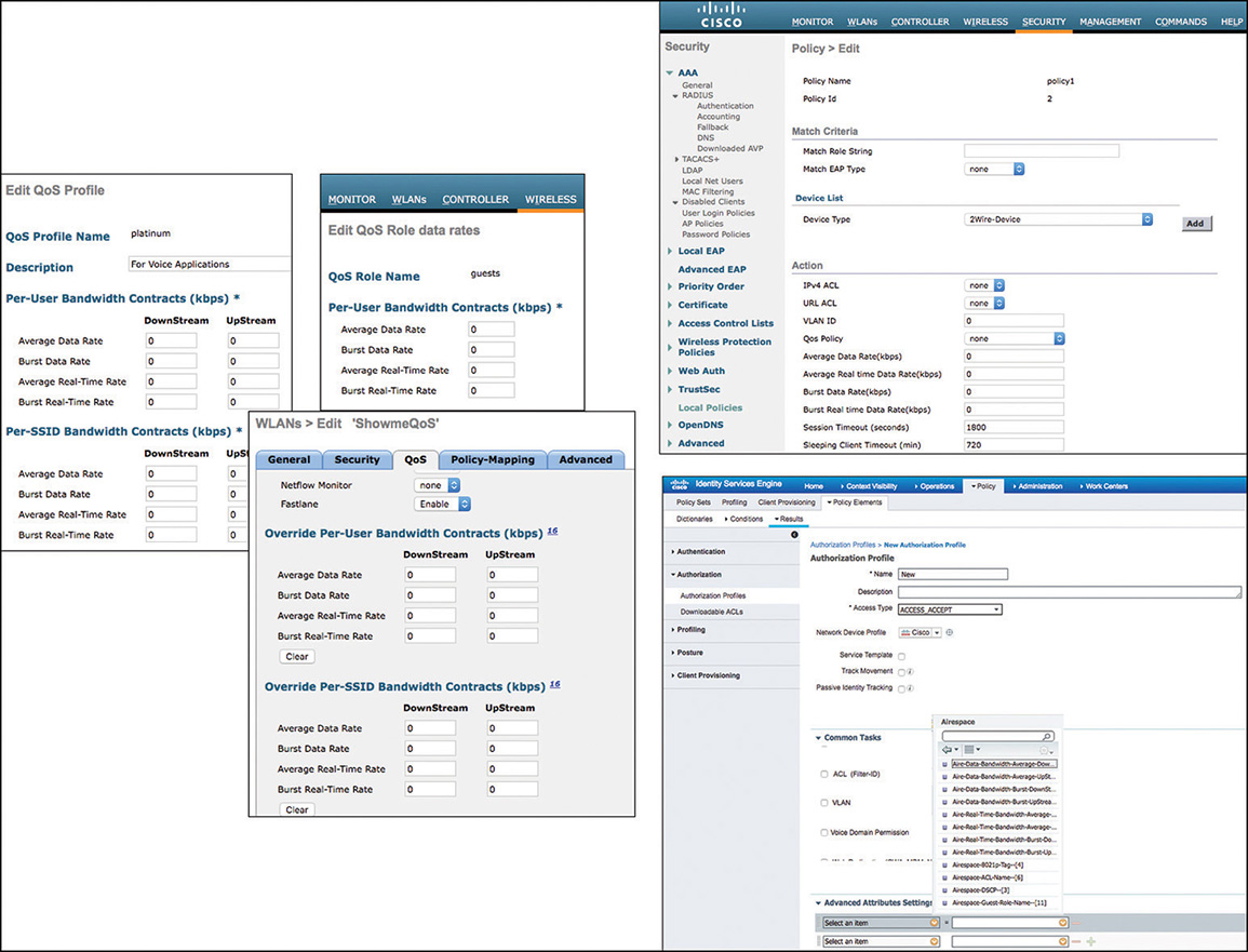
When several contracts are possible for a given user, the most targeted and most restrictive configuration applies. Configurations are looked at in this order: AAA user-specific configuration first; then device local policy; then guest role if applicable; then WLAN contract; and last, QoS profile contract. The QoS profile contract is applied only if no other contract was defined.
If one or multiple QoS contracts were defined outside the QoS profile and are applicable for a given user (in the WLAN, local policy, guest role, or AAA), the QoS profile contract is ignored for the user for which these non-QoS-profile contracts apply. In other words, if your QoS profile contract is 10 kbps, but the user matches a local policy restricting to 50 kbps, that user will receive 50 kbps.
Also, AAA always overrides local configs. If your WLAN BW contract is 10 kbps but AAA applies 50 kbps for a given user, that user receives 50 kbps.
Finally, local policies override roles.
These combinations may look complex. You should understand the various ways of creating bandwidth contracts, in case the CCIE Wireless exam asks you to configure such a contract. However, it is clear to all that bandwidth contracts are not best practices. Although there may be an ask and a need to configure a contract for specific users, no reasonable design would mandate contradicting contracts for various user types with the requirements to map the various possible overlaps in order to decide which contract a user eventually receives. If this scenario occurs, you should suggest to your customer a better network design. If you still have to face this unfortunate scenario, you can always verify which bandwidth contract is being applied to a given user with the show client detail command. There, you will be able to see which contract overrode the others and was applied to your test client.
For corporate WLANs, where voice is expected, Platinum is the recommended QoS profile. After you pick a QoS profile, you associate it to the WLAN from the QoS tab (CLI config wlan qos). For corporate WLANs and Platinum profiles, as much as possible, bandwidth contracts should not be used. Maximum priority should be set to voice. Unicast default priority and multicast default priority should be set to best effort, and Wired QoS protocol should be set to none, as represented in Figure 7-20. In the CLI, all these elements are configured with the family of command config qos.
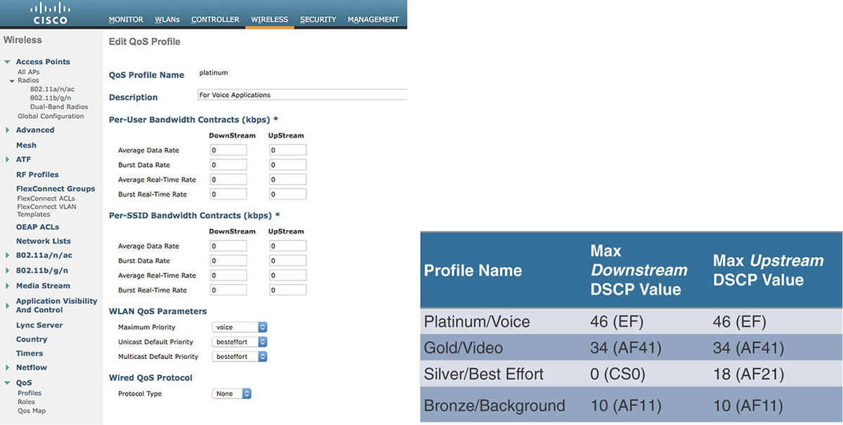
The reason for not using bandwidth contract was explained in the previous section: as much as possible, it is better to use QoS marking to create differentiated treatment for applications. Using bandwidth contracts creates artificial static limits that do not take into account the traffic type, the user location (close or far from the AP), and the general available airtime in the cell.
The maximum priority is the effective ceiling of the profile. You should remember that this ceiling is expressed as an 802.11e AC (voice, video, best effort, and background). This means that the maximum priority is intended for the wireless space, not the wired space (although it has an effect on the wire, as we’ll see later). This ceiling means that no traffic will be marked higher than voice downstream from the AP (for any SSID to which this QoS profile is associated).
Unicast Default priority represents the QoS marking for non-WMM stations. In other words, when traffic arrives from the wire for a station that does not support WMM (and therefore does not support 802.11e QoS), how should you treat that traffic on the AP? The legacy recommendation was to treat the traffic as representative of the QoS profile category. In other words, if you associated a Platinum profile to an SSID, the assumption was that most traffic for that SSID was likely to be Platinum (that is, voice). Therefore, treating all traffic by default as voice was the rule. This was back in the days when admins used to configure specialized SSIDs (for example, Voice SSID, Data SSID), and when devices were also specialized (your voice devices would all be hard phones). Times have changed. Today, you configure general SSIDs (corporate, with all sorts of traffic, voice and others), and devices are generic (BYODs run voice applications and data applications). As a consequence, you do not expect anymore that an unknown device that does not support QoS would primarily be a voice device in such a generic SSID. As WMM support is mandatory for 802.11n/ac, no WMM support is equivalent to “old legacy device.” This is unlikely to be your choice for voice traffic. It is probably an old laptop, a barcode scanner, or some other non-voice device. As a consequence, traffic to this non-WMM device should be best effort.
Multicast can be any type of traffic; however, it is a problematic type of traffic because it is addressed to multiple recipients. This means that the targets may be on a given AP radio but in different WLANs. It is therefore difficult to decide whether a particular priority should be given to multicast (over the air, but also between the WLC and the AP). A general rule is to treat this traffic as “generic” (best effort). However, if you know of a particular multicast traffic that critically needs specific QoS treatment, an exception can be made (and the multicast default priority can be changed accordingly).
The Wired QoS protocol relates to the CAPWAP encapsulation between the WLC and the AP. The QoS profile acts as a ceiling. This notion is not visible with Platinum because the ceiling is at the highest QoS marking. So let’s take Gold as an example, to better visualize the consequences of that ceiling concept. Please note that in most real-world environments (and the CCIE lab is not a real-world environment), you will not use Gold anymore, but this profile serves as a useful intermediary between the highest ceiling (voice) and best effort.
When a packet comes into the WLC, coming from the wired side and destined for a wireless client, in a WLAN associated to a specific QoS profile (in this case Gold), the WLC will first look up the client. We suppose here that AVC is not configured. The WLC will then look at the QoS profile associated with that client (Gold). Suppose that the incoming packet has a DSCP marking of 46 (EF), as represented in Figure 7-21.
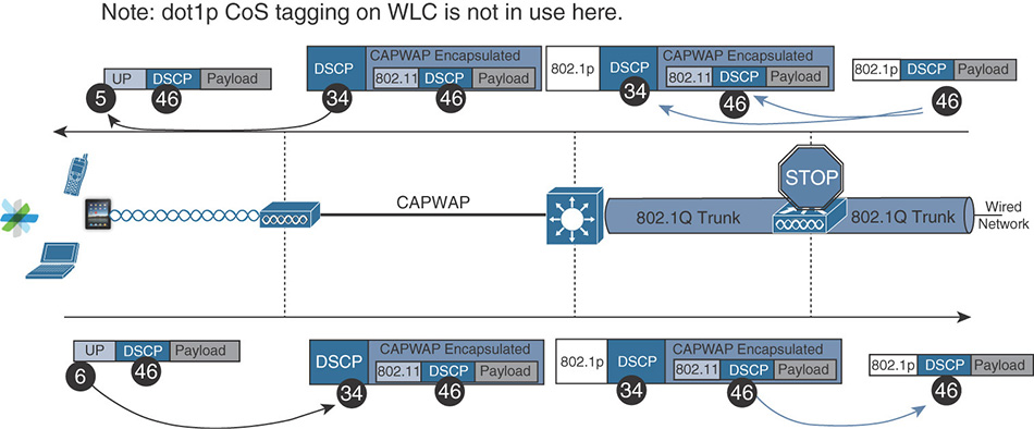
The WLC is going to convert the 802.3 header into an 802.11 header, then encapsulate the 802.11 frame into a CAPWAP header. The DSCP value, inside the encapsulated CAPWAP packet, is unchanged (46); however, the Gold profile creates a QoS ceiling of AF 41 (DSCP 34). Therefore, the WLC is going to cap the CAPWAP outer IP header to DSCP 34. In this example, because the Wired QoS profile is set to none, the 802.1p (Layer 2 QoS over the Ethernet link) is ignored and left at 0. Using DSCP is the recommended practice. Therefore, Wired QoS is expected to be left to None.
Note
In older codes (before 7.x), the outer DSCP header would be left untouched (DSCP 46), and only the 802.1p value would be capped (802.1p 4 in the case of Gold/video). In those days, you needed to enable Wired QoS profile and set it to the proper ceiling, 4. This task was made complex by the fact that some codes actually displayed the 802.11e equivalent (i.e., “5” for video, because this is the UP for video) instead of displaying directly the 802.1p value. This complexity was removed since, and what you see in AireOS 8.x and later is indeed the 802.1p direct value.
However, AireOS 8.x and later also cap the outer DSCP value, which is required in a world where using DSCP is recommended. Therefore, the 802.1p and Wired QoS protocol configuration has become obsolete, and you would only use it in older networks where DSCP is not supported on the switching infrastructure.
The CAPWAP encapsulated packet is then going to transit toward the AP. The AP is likely to be on an access port (not a trunk port), so there is no 802.1p value on that last hop. (Remember that the 802.1p field is in the 802.1Q section of the header, and therefore is present only on trunk links.) Upon receiving the packet, the AP is going to look at the outer DSCP value and compare it to the QoS ceiling (Gold) associated to the target client WLAN. This two-step process is important because it has two consequences:
The AP never looks at the inner DSCP value.
If you change the outer DSCP on the way between the WLC and the AP (by using remarking on one switch), you are going to change the treatment of that packet over the air, regardless of what initial QoS value was set by the wired client or the WLC.
If the CAPWAP outer DSCP value is equal to or lower than the QoS ceiling, the AP sends the packet with the requested QoS value. If the outer DSCP value is higher than the ceiling, the AP sends at the ceiling level. Let’s take a few examples. Suppose the outer DSCP is AF11 (background). This is lower than the Gold ceiling, therefore the AP sends the packet in the background queue (AC_BK, UP1), as requested by the outer DSCP value (AF 11). Suppose now that the outer DSCP is AF41. This is right at the ceiling level and still allowed. The AP sends the packet in the video queue (AC_VI, UP5), as requested by the outer DSCP value (DSCP 34, AF 41). Suppose now that the packet outer DSCP was remarked on the way to EF (DSCP 46). Remarking on the path is the only possible explanation, as the WLC already capped the outer header to DSCP 34 (AF 41), so the packet should not get a DSCP 34 without some equipment changing the marking on the path. In any case, the AP sees that DSCP 46 is higher than the ceiling (34), and therefore positions the packet in the ceiling queue, AC_VI, UP 5. This UP treatment decides the frame priority between the AP and the client. Inside the frame, the payload DSCP is still 46.
The same logic applies for upstream traffic. Suppose that the wireless station sends a frame marked UP6 (AC_VO) and DSCP 46. This is possible, even if the QoS ceiling is Video. The QoS ceiling is an infrastructure configuration, not a behavior dictated by the AP to its clients. Upon receiving the frame, the AP is going to encapsulate the 802.11 frame into CAPWAP and look at the UP value. This occurs if you use the default behavior of using the UP upstream. As we’ll see shortly, you should change the defaults and use Trust DSCP instead. In that case, the AP would look at the DSCP value and ignore the UP value. The process logic is the same, only the field considered changes. As the value exceeds the Gold ceiling, the AP caps the CAPWAP outer DSCP header to Gold (AF 41) and sends the packet to the WLC. The WLC then decapsulates the packet, converts the 802.11 frame into an 802.3 frame, then sends it to the wire without changing the requested DSCP value (46).
This process may look complex, and it may seem that the treatment by the WLC is not the same upstream and downstream. This appearance is an illusion. An easy rule to remember is that the WLC or the AP never touch the requested inner DSCP value. If you give the system, in any direction, a packet with a given DSCP value, you will receive a packet with that DSCP value unchanged on the other side of the system. The WLC-AP pair only controls the CAPWAP header value and the L2 QoS treatment over the air, downstream. However, you should keep in mind that intermediate devices between your APs and WLCs (switches, routers) will prioritize the packets based on the outer CAPWAP header QoS tag. These devices may also rewrite this tag based on their local QoS policies. This behavior means that the QoS tag initially written on the outer CAPWAP header by one end (WLC or AP) may be different when the packet reaches the other end (AP or WLC). Upstream, this possible change affects only the priority of the packet between the AP and the WLC (the WLC looks at the inner QoS tag to decide the packet fate). Downstream, this possible change affects both the priority of the packet between the WLC and the AP and the priority of the packet over the air (because the AP uses the outer CAPWAP QoS value to decide the downstream UP queue and value). The logic of this asymmetry is that you control the WLC-AP-client space. If a switch is between the WLC and the AP, it is under your administrative control. If that switch rewrites the outer CAPWAP QoS, it is because you have decided a particular mapping policy for that QoS value. That policy should be enforced. However, the space beyond the WLC (upstream) is not your domain anymore; you should return to that space the QoS tags unchanged, leaving the decision to keep or rewrite these tags to the LAN admin.
The QoS control mechanism becomes a bit more complex when your incoming wired packet has an unexpected QoS value (something that is not a clear voice or video marking). On the wire, the rule is simple. If the requested DSCP marking is below the ceiling, it is translated unchanged to the CAPWAP outer DSCP value. But what happens over the air, where there are at most only eight values? QoS mapping recommendations have been evolving over time (as you may remember from the first section of this chapter), and the AireOS code that you will get at the CCIE exam does not always reflect the latest recommendations. This is not an issue, as a macro will help you to configure the right mapping, but you may want to be aware of AireOS defaults, in case you decide to not configure anything.
The logic of the internal mapping is to select key DSCP values that have a special significance (voice, and so on) and create a special mapping for these values. These are the values we took as examples earlier. Then, any other value is a simple mapping between the three MSB (the IP Precedence bits) to UP, and vice versa.
Default QoS Mapping
Note
You will find online multiple documents that show you the QoS mapping for AireOS. Depending on when this document was written, it can be pretty close to the current (on AireOS 8.3 and later) mapping, or very far. Do not waste time trying to decide who is right and who is wrong. Most of the time, the difference is when the document was written, not so much about whether the author knew how to measure QoS.
Table 7-5 shows the current (AireOS 8.3 and later) default mapping:
Table 7-5 AireOS Default DSCP-UP Mapping
Downstream Wired DSCP |
PHB |
Binary |
Air UP |
3mb |
Notes |
0 |
000000 |
0 |
0 |
||
1 |
000001 |
0 |
0 |
||
2 |
000010 |
1 |
0 |
||
3 |
000011 |
0 |
0 |
||
4 |
000100 |
1 |
0 |
||
5 |
000101 |
0 |
0 |
||
6 |
000110 |
1 |
0 |
||
7 |
000111 |
0 |
0 |
||
8 |
cs1 |
001000 |
1 |
1 |
|
9 |
001001 |
1 |
1 |
||
10 |
af11 |
001010 |
2 |
1 |
|
11 |
001011 |
1 |
1 |
||
12 |
af12 |
001100 |
2 |
1 |
|
13 |
001101 |
1 |
1 |
||
14 |
af13 |
001110 |
2 |
1 |
|
15 |
001111 |
1 |
1 |
||
16 |
cs2 |
010000 |
2 |
2 |
|
17 |
010001 |
2 |
2 |
||
18 |
af21 |
010010 |
3 |
2 |
|
19 |
010011 |
2 |
2 |
||
20 |
af22 |
010100 |
3 |
2 |
|
21 |
010101 |
2 |
2 |
||
22 |
af23 |
010110 |
3 |
2 |
|
23 |
010111 |
2 |
2 |
||
24 |
cs3 |
011000 |
3 |
3 |
Should be UP 4 |
25 |
011001 |
3 |
3 |
||
26 |
af31 |
011010 |
4 |
3 |
|
27 |
011011 |
3 |
3 |
||
28 |
af32 |
011100 |
3 |
3 |
Should be UP 4 |
29 |
011101 |
3 |
3 |
||
30 |
af33 |
011110 |
3 |
3 |
Should be UP 4 |
31 |
011111 |
3 |
3 |
||
32 |
cs4 |
100000 |
4 |
4 |
|
33 |
100001 |
4 |
4 |
||
34 |
af41 |
100010 |
5 |
4 |
|
35 |
100011 |
4 |
4 |
||
36 |
af42 |
100100 |
4 |
4 |
Should be UP 5 |
37 |
100101 |
4 |
4 |
||
38 |
af43 |
100110 |
4 |
4 |
Should be UP 5 |
39 |
100111 |
4 |
4 |
||
40 |
cs5 |
101000 |
5 |
5 |
|
41 |
101001 |
5 |
5 |
||
42 |
101010 |
5 |
5 |
||
43 |
101011 |
5 |
5 |
||
44 |
voice admit |
101100 |
5 |
5 |
Should be UP 6 |
45 |
101101 |
5 |
5 |
||
46 |
ef |
101110 |
6 |
5 |
|
47 |
101111 |
6 |
5 |
Should be UP 5 |
|
48 |
cs6 |
110000 |
6 |
6 |
|
49 |
110001 |
6 |
6 |
||
50 |
110010 |
6 |
6 |
||
51 |
110011 |
6 |
6 |
||
52 |
110100 |
6 |
6 |
||
53 |
110101 |
6 |
6 |
||
54 |
110110 |
6 |
6 |
||
55 |
110111 |
6 |
6 |
||
56 |
cs7 |
111000 |
6 |
7 |
|
57 |
111001 |
6 |
7 |
||
58 |
111010 |
6 |
7 |
||
59 |
111011 |
6 |
7 |
||
60 |
111100 |
6 |
7 |
||
61 |
111101 |
6 |
7 |
||
62 |
111110 |
6 |
7 |
||
63 |
111111 |
6 |
7 |
You see that a few values are highlighted, because the defaults do not match the best practices. They are legacy recommendations. However, using defaults is also not the best practice, because the defaults are based on the idea that you would use UP to DSCP mapping upstream, which you should not do in most cases. So there is an expectation that you are going to override these defaults anyway (even if you use UP upstream). Therefore, there is not a strong incentive to change the AireOS code to hard code different default values (because you won’t use these defaults anyway, whatever they are, because they assume “trust UP” to comply with backward compatibility rules).
DSCP Trust and 802.11u QoS Maps
Since AireOS 8.1MR1, you can create a custom DSCP to UP and UP to DSCP map. An optimized version of this custom map can be created with a simple macro (Fastlane, examined later in this section). However, you may want to understand the custom map command and structure, in case you need to customize it by hand. The customization page is a global setting (applies to all SSIDs and all bands) and is configured from Wireless > QOS > QoS map, as shown in Figure 7-22.
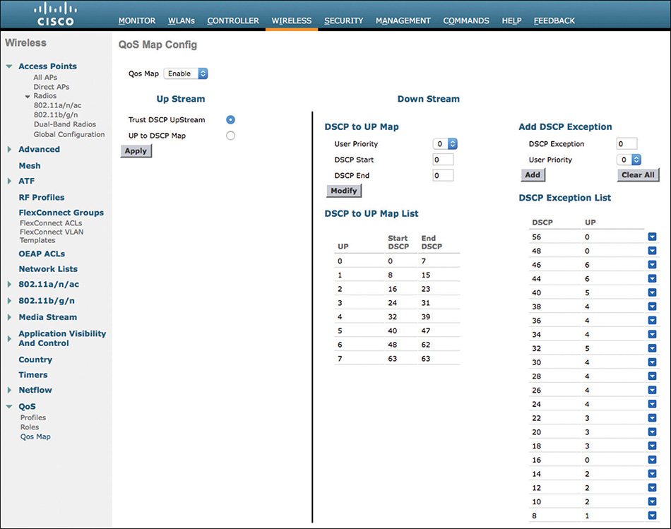
From this page, you can set three configuration items:
Enable DSCP trust from the client
Configure a custom DSCP to UP map (called exceptions)
Configure a custom UP to DSCP map
The recommended practice is to trust DSCP upstream. When this function is activated, the AP looks at the DSCP field in the frames coming from wireless clients (instead of looking at the UP). As detailed in the first part of this chapter, and shown in Figure 7-23, using DSCP instead of UP allows for a richer translation of QoS intents between mediums.
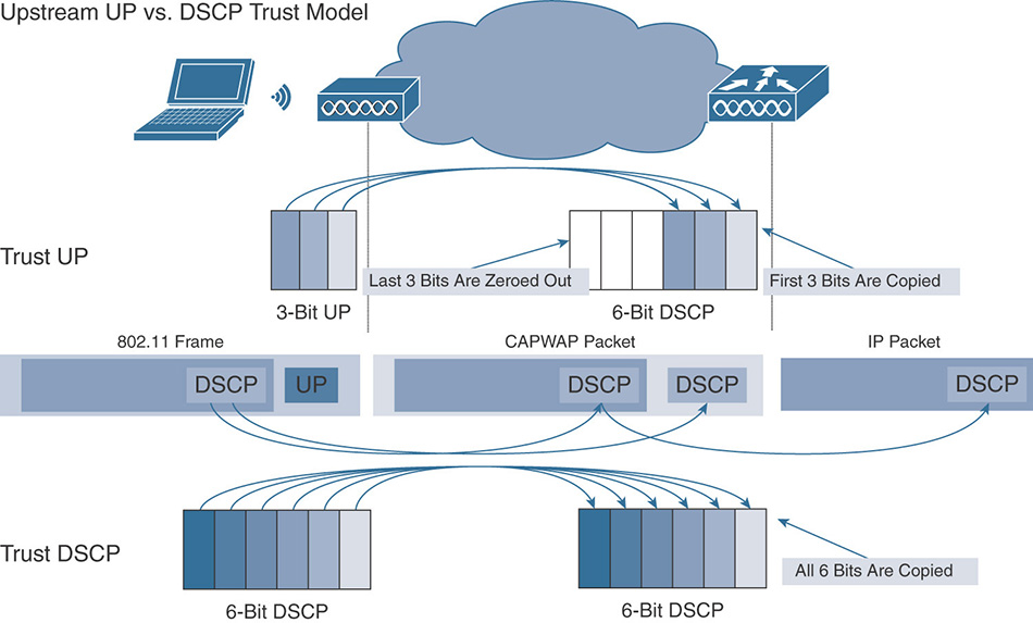
You can directly use the end-to-end intent for that packet, instead of using a 3-bit local L2 Wi-Fi QoS intent to express intent across another medium (Ethernet) and possible routing hops, where DSCP is more meaningful than Layer 2 values. Keep in mind that the action of the AP does not change. Whether you trust DSCP or trust UP upstream, the AP still looks at the incoming value (DSCP or UP), compares it to the WLAN QoS ceiling expressed through the associated QoS profile, and uses this comparison to either copy the requested DSCP value (or UP value) to the CAPWAP outer header DSCP section (using direct copy in case of DSCP trust, or using a UP to DSCP map in case of UP trust).
Therefore, the recommended practice is to enable DSCP trust upstream by checking the corresponding check box on the QoS map configuration page. From the CLI, the equivalent is config qos qosmap trust-dscp-upstream enable. You would trust UP only if the majority of your wireless clients are unable to mark DSCP but would mark UP. However, this would be an uncommon scenario.
You can also configure customized DSCP to UP and UP to DSCP maps. In the CLI, the structure of the command is confusing, and shown in Figure 7-24.
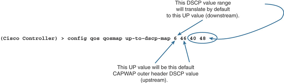
This complexity is reflected in the UI in AireOS 8.3 code as shown in Figure 7-22. In AireOS 8.4 and later, this direct translation of the CLI was replaced by an intent-oriented display, and DSCP to UP was separated from UP to DSCP. The reason for the complexity comes from the fact that the command is a direct translation from 802.11u. This amendment, published in 2011, contains multiple provisions for HotSpot 2.0. In a context where Trusting UP was the norm (with all the limitations expressed earlier that were well known to QoS experts working on 802.11u), 802.11u allowed the AP to send to the client station an UP to DSCP map. This could be used by the station to set the best UP for the upstream transmission, knowing the intended DSCP for a given traffic. In other words, if you want to send a video packet, if you know that video receives AF 41 in your internal client operating system, and if you want to make sure that the AP, trusting UP, assigns AF 41 to your packet, you have to look at the UP to DSCP map, find which UP receives AF 41, and “simply” assign that UP to your upstream video packet.
However, there was a need to also express a DSCP to UP map. The intent was to tell the station “if your operating system can only generate DSCP, and you are not sure about the best UP for each DSCP, here is the DSCP to UP map recommended for this network.” A natural push in the 802.11u group was to argue that such a map was unnecessary, because the station could use the UP to DSCP map in reverse: if UP 5 is AF 41, then AF 41 should be UP 5. Of course, this approach was seen as too simplistic by many because this logic works only for 8 DSCP values (those that match each of the 8 UP values in the UP to DSCP map). For example, if the UP to DSCP maps states that AF 41 (DSCP 34) is 5, and EF (DSCP 46) is 6, what is the UP value of DSCP 36? Some proponents of simplification suggested to use an UP to DSCP range. In other words, instead of just stating “UP 6 is DSCP 46,” the map would state “UP 6 is DSCP 44 to 46.” Creating such a range also implies creating defaults. If I have UP 6 for my frame, which DSCP should I put—DSCP 44, 45, or DSCP 46? As a result of these discussions, the UP to DSCP map transformed into a UP to DSCP range, with a default UP to DSCP map, if you only have UP to start from. This already makes the command a bit complicated, but these arrangements still did not satisfy all the requirements, for the simple reasons explained in the first section of this chapter. For most UP values, a simple 3 MSB translation works (CS 3 is 011 00 0, which can be simply translated as UP 3, also 011). But quite a few UPs and DSCP require special mapping (like Voice 101 11 0, which would be UP 5 but should in fact be UP 6). As a consequence, 802.11u also allowed a series of “exceptions” to be defined (DSCP values that would translate to special UP values, without using the standard UP to DSCP range map). Because there are really 21 DSCP values in use (as per RFC 4594), the exception list can contain up to 21 entries.
This complexity in 802.11u is directly translated into the CLI command, which is built in two parts: an UP to DSCP range and a DSCP to UP exception.
The UP to DSCP range section is configured on the left side of the QoS map UI screen, and with the command shown in Figure 7-24: config qos qosmap up-to-dscp-map. With this command, you start by calling the target UP value (for example, config qos qosmap up-to-dscp-map 1, to configure the map for UP 1). You then configure the default DSCP value for this UP (config qos qosmap up-to-dscp-map 1 8, to express that DSCP 8, or CS1, should be the DSCP to which UP 8 should map, if we have only UP to work from). You then add the range for which this UP is valid (for example, config qos qosmap up-to-dscp-map 1 8 8 15, to express that if we have a DSCP value and we are looking for the UP, then UP 1 should be chosen for any DSCP value between 8 [CS1] and 15 [15 is unused, but includes DSCP 14, or AF 13]).
Sounds complicated? Yes, it is. The matter is made worse by the fact that you must configure each UP (you cannot configure a map for UPs 1 to 6 and skip 7), and also by the fact that the ranges cannot overlap (you cannot map UP 1 to DSCP 8 to 24, and map UP 2 to DSCP 24 to 32, because the system would not know the right UP for DSCP 24). Also, this mapping is very logical in the case of 802.11u, but in an AireOS controller, you are not trying to tell the wireless station what to do (at the time of writing of this section, no client makes use of the 802.11u QoS map); you are trying to tell your AP how to translate between UP and DSCP, and vice versa. And if you trust DSCP upstream, why would you care about an UP to DSCP map (you are using DSCP, not UP)? Yet the command mandates that you tell the system about the map (because the map will be advertised by the AP, as per 802.11u).
The real part of the command you care about is the DSCP to UP “exception” section. This is useful downstream. When you receive wired packets with a DSCP value, the QoS profile will still determine the ceiling, as usual. However, if your DSCP value is below the max value (QoS profile ceiling), should you use the default DSCP to UP 3 MSB map or a special DSCP to UP translation? The right part of the QoS map configuration screen and the config qos qosmap dscp-to-up-exception allow you to configure up to 21 DSCP to UP special mappings. This is something you should configure if you trust DSCP upstream.
Luckily (see the “Fastlane Configuration and Client Behavior” section later in this chapter), there is a macro to configure all the right “recommended” values in one single command shown later in Figure 7-36. However, you should understand the values that this macro sets and what these recommended values are:
config qos qosmap up-to-dscp-map 0 0 0 7
config qos qosmap up-to-dscp-map 1 8 8 15
config qos qosmap up-to-dscp-map 2 16 16 23
config qos qosmap up-to-dscp-map 3 24 24 31
config qos qosmap up-to-dscp-map 4 32 32 39
config qos qosmap up-to-dscp-map 5 34 40 47
config qos qosmap up-to-dscp-map 6 46 48 62
config qos qosmap up-to-dscp-map 7 56 63 63
config qos qosmap dscp-to-up-exception 48 0
config qos qosmap dscp-to-up-exception 56 0
config qos qosmap dscp-to-up-exception 46 6
config qos qosmap dscp-to-up-exception 44 6
config qos qosmap dscp-to-up-exception 40 5
config qos qosmap dscp-to-up-exception 38 4
config qos qosmap dscp-to-up-exception 36 4
config qos qosmap dscp-to-up-exception 34 4
config qos qosmap dscp-to-up-exception 32 5
config qos qosmap dscp-to-up-exception 30 4
config qos qosmap dscp-to-up-exception 28 4
config qos qosmap dscp-to-up-exception 26 4
config qos qosmap dscp-to-up-exception 24 4
config qos qosmap dscp-to-up-exception 22 3
config qos qosmap dscp-to-up-exception 20 3
config qos qosmap dscp-to-up-exception 18 3
config qos qosmap dscp-to-up-exception 16 0
config qos qosmap dscp-to-up-exception 14 2
config qos qosmap dscp-to-up-exception 12 2
config qos qosmap dscp-to-up-exception 10 2
config qos qosmap dscp-to-up-exception 8 1
config qos qosmap trust-dscp-upstream enable
config qos qosmap enable
The UP to DSCP part sets UP 0, 1, 2, 3, 4, 5, 6, and 7 to default DSCP 0, 8 (CS1), 16 (CS2), 24 (CS3), 32 (CS4), 34 (AF41), 46 (EF), and CS7, respectively. In other words, the defaults are to use the 3 MSBs, translating each up to the corresponding CS value, with the exception of video (UP 5, AF 41) and voice (UP 6, EF). The corresponding ranges are also set the same way, with the same exception. For example, UP 1 covers all DSCPs between CS 1 (001 00 0) and the CS 2 lower boundary (001 11 0, which is DSCP 14, a possible value, but also 001 11 1, DSCP 15, which should not be present in a network but is in theory possible). The same logic applies for the other UPs. UP 4 covers the same way all DSCPs from 100 00 0 (DSCP 32, CS4) to 100 11 1 (unlikely DSCP 39, but also includes AF 43, DSCP 38). However, a special exception is made for AF 41, which is the default map for UP 5. This exception means that AF41 somewhat “jumps one range up” (AF 41 is 100 01 0 but translates to a 101 UP binary). However, AF 41 is an exception, and UP 5 maps otherwise to the other 101 DSCP values (101 00 0, CS 5 or DSCP 40, to 101 11 1, which includes 101 11 0, DSCP 46 or EF, still in the 101 range).
Because voice is special, an exception is made again, where UP 6 maps by default to EF, thus overriding again the general range. Anything above 101 11 0 (EF) is network control and should not be present in an access network. However, as explained in the first part of this chapter, you may find contexts where such values are permitted. In this case, they should map to UP 6. This is what the 6 46 48 62 expresses. The only exception is the reserved value CS 7/UP 7. This value would exist only by itself, and if a special “highest override” experimental value of 111 11 1 was seen.
The DSCP to UP exception command then lists all the well-known and expected DSCP values and maps them to their recommended UP value, as shown earlier in Figure 7-8. Notice that these recommendations span most of the UP values. You will find that most systems (outside of Cisco) use only four ACs, and therefore only four UPs. By contrast, AireOS uses the full span of UP possibilities.
EDCA Parameters
Another best practice set of parameters that you may want to change are the EDCA parameters, in Wireless > 802.11a/n/ac (or 802.11b/g/n) > EDCA Parameters (CLI config advanced 802.11a / 802.11b edca-parameter). The default value is WMM, which matches the 802.11e standard recommendations for EDCA. You may have some cases where the band is primarily designed for a specific traffic type. Several other types of EDCA values are possible, as shown in Figure 7-25.
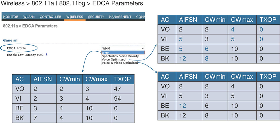
The blue color shows the changes from the standard WMM profile. Voice Optimized increases the AIFSN for all queues except voice, and also increases some CWmin and CWmax values. Note that Voice Optimized also sets the TXOP for voice and video to 0. This change fulfills two purposes:
As explained at the beginning of this chapter, a TXOP value offers transmit opportunities but also limits the transmit duration. A value of 0 allows only one frame per service period but also allows that frame to be the max duration allowed by the protocol. With 0, voice and video can send large blocks, just like the other queues.
Some drivers (especially on hard phones) queue frames in a peculiar way. The software part of the phone decides whether the packet needs to be sent to the queue, then subcontracts the transmit part to the driver. The driver then looks at the TXOP and decides on the number of frames that should be sent in the next service period. The frame burst is built, and the phone waits to get medium access. When the access is granted, the entire burst is sent. But this logic does not account for losses and delays. If delays appear, the software part of the phone may decide to skip a packet and send the next one instead, privileging real-time over audio quality (a slightly metallic texture of the sound, due to a packet missing here and there, is better than no audio at all because the buffer is empty). However, with the mechanism previously described, when a frame is in the next burst in the drive, it is too late. The software can’t drop a packet here and there to put later packets instead. The result is a higher risk of empty buffer and dead air. Setting the TXOP to 0 compensates for these hard phone behaviors, making sure that only one packet at a time gets sent to the driver.
In most cases, you would not choose the default WMM value but the Fastlane value instead, for which AIFSN and CW values are shown in Figure 7-14. However, there may be cases where you are given very specific requirements that would push your choice to another set of optimized EDCA parameters.
WLAN and WMM Configurations
At this point, you have configured your QoS profiles, you likely have chosen to trust DSCP upstream, and you have set your DSCP to UP and UP to DSCP maps. You have also chosen the best EDCA parameter set. All this configuration relates to QoS, which means that your clients are expected to have some support of QoS. In Wi-Fi terms, this means that they support WMM. If they are 802.11n or 802.11ac compliant, they must support WMM, so it is likely that most of your enterprise clients will be in this category.
Your next step is to go to the WLAN QoS tab and associate the right QoS profile: Platinum for an enterprise hybrid BYOD WLAN, where voice is expected, as shown in Figure 7-26, and Best Effort or Background for a guest WLAN.
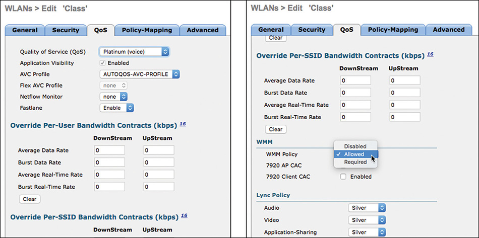
Lower down the QoS tab, set WMM to Allowed or Required. If your stations support 802.11n or 802.11ac, they support WMM, and setting WMM to Required is the right choice. The Required option was especially useful for smartphones. Many of them would prefer Best Effort and would enable WMM only if the cell mandates it. In other words, set WMM to Allowed (allowing both WMM and non-WMM devices and behavior), and these smartphones would not activate WMM. Set WMM to Required, and these smartphones would activate WMM (because they have no choice). Because WMM also activates QoS, WMM is much preferred over best effort. Using WMM Required was a way to enforce this support.
However, using WMM Required means that non-WMM devices cannot join the WLAN (the devices that do not support WMM, not the devices that would support it but are too lazy to activate it by themselves). If you have such devices in your network, and you cannot upgrade them to newer devices, you may have to set WMM to Allowed.
CAC Configuration
The next parameter to consider is Call Admission Control. Recall that this is Wireless CAC, not Unified Communications CAC. It is configured per band in Wireless > 802.11a/n/ac | 802.11b/g/n > Media as shown in Figure 7-27 (CLI config 802.11b|802.11a cac).
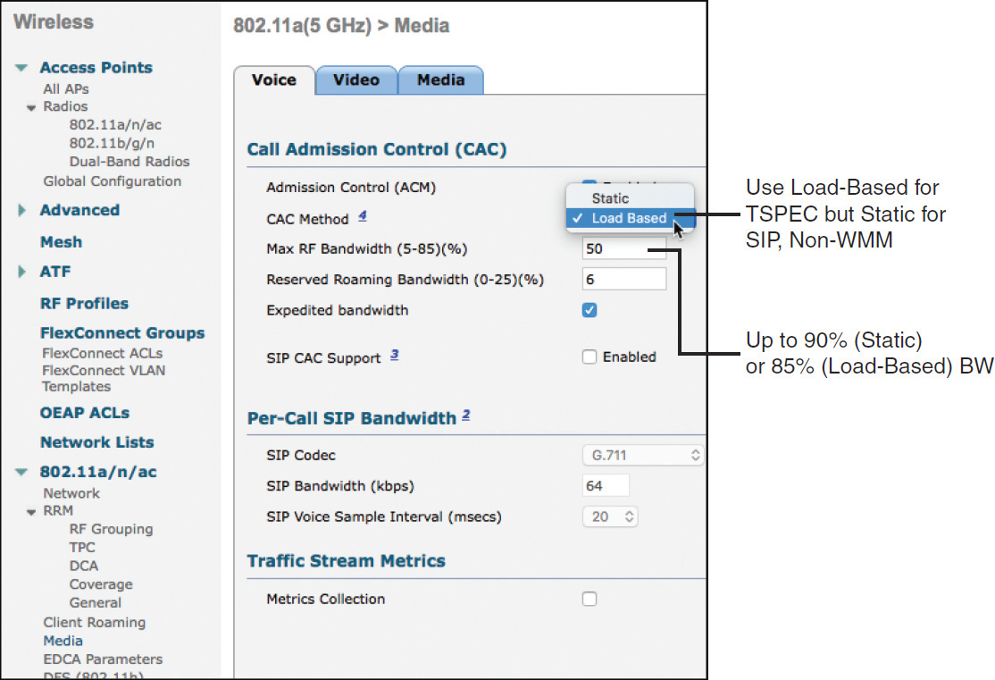
Voice CAC, protecting UP 6, is enabled by checking the ACM Enabled check box on the Voice tab. The choice to check this option depends on your voice client population. Most hard phones will support TSPEC (as described in the first part of this chapter). iOS 10 and later are “immune” to Voice ACM (see the “FastLane Configuration and Client Behavior” section). However, the vast majority of the other smartphones will not support TSPEC and will therefore be unable to send traffic in the UP 6 queue. This will force your smartphones to revert to either UP 5 or UP 0. This reversion scheme is mandated and tested by the WMM certification (if the Voice ACM bit is on, phones must send voice traffic in either UP 5 or UP 0). You need to test your phone population to validate their behavior and choose the configuration most advantageous to clients:
If your phones support TSPEC, Voice ACM is a good feature in your network.
If your phones and tablets are iOS 10 and later, and laptops Mac OS 10.13 or later, Voice ACM is a good feature in your network.
If your phones, tablets, and laptops do not mark UP 6 for voice in the first place (because the apps do not mark QoS, or because the app marks a DSCP value that does not translate to UP 6 when the phone sends), ACM is neutral for these clients.
If your phones, tablets, and laptops do mark UP 6 when sending voice app traffic, ACM is a limitation for these clients.
The fact that clients have to revert to UP 5 or UP 0 only represents the upstream part of the constraint. When the AP receives the frame, it uses the UP or DSCP value for the upstream part of the journey. If the AP uses UP, the UP 5 or UP 0 would result in worse treatment than expected for that voice packet. This is another reason why trusting DSCP is better if the upstream packet also includes the correct DSCP value for voice. Although WMM mandates that the UP would be lower, the DSCP would be unchanged by the ACM configuration.
As for the return traffic, and as shown in Figure 7-28, the infrastructure is aware that ACM is enabled. Although your profile may be Platinum, therefore allowing up to voice (EF) traffic, the ACM bit will limit this ceiling over the air. If the return traffic (from the wire, toward the client) is also voice, with a DSCP 46 marking, the WLC to AP segment of the network will carry the DSCP 46 value, but the AP will check whether the target client did undergo the ADDTS choreography. If the client is not in the ACM-allowed list, the AP will send the frame over the air as Best Effort.
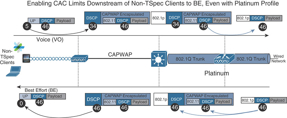
You should be aware that this feature works exactly as intended. Its purpose is to limit the voice queue only to clients that are actually sending voice. They should describe their traffic first. The exceptions are iOS and MacOS devices (see the “FastLane Configuration and Client Behavior” section), because there is high certainty that traffic sent from these devices in UP 6 queue is indeed going to be voice. The ACM feature limits the ability of, say, Linux BitTorrent users, from using the highest priority queue for traffic that has nothing to do with voice. However, in a controlled environment where you trust your client population and some devices may need access to this queue without the possibility of TSPEC, this feature may be a limiting factor and should therefore not be enabled.
Note
These recommendations apply to Voice ACM. Video ACM is altogether different. Although WMM allows the same ACM principles for the video queue, there is in fact no client on the market that supports Video ACM. Although there is a Video tab where ACM for UP 5 can be configured, you should always keep Video ACM disabled in real life. The only case where Video ACM should be enabled is if you have experimental clients that support Video ACM, or if you are in a lab environment where your knowledge of Video ACM is tested.
If you enable Voice ACM, you can choose the static or load-based method of evaluating the available bandwidth on each AP radio where a WLAN with WMM is configured, and with clients trying to send traffic in the Voice AC. Static is the old method, where only the AP clients traffic was considered. Load based is the newer method that accounts not only for the AP clients but also for the general activity on the channel (neighboring APs and clients on the same channel that also consume airtime, even if they are not clients of the local AP radio). You should always choose load based. You will find some old documentation that states that static is still needed when SIP CAC is configured (details following), but this is old documentation that needs updating. SIP CAC also leverages load-based CAC today, so there is no reason to use the static method anymore.
Regardless of the CAC method you choose, you can then configure the Max RF Bandwidth allocated to this reserved voice traffic. When performing ACM, the AP will calculate the current channel load, then evaluate the added load described in the ADDTS request. If the requested flow brings the channel load above the value configured in Max RF Bandwidth, the ADDTS request receives a reject response.
The default value for Max RF Bandwidth is 75%, which matches a large cell dedicated to voice traffic. In most enterprise environments, cells are small. A consequence of this size reduction is that the airtime consumed by a voice call will be less. Also, most enterprise environments have hybrid WLANs, where voice traffic coexists with data traffic. It is unusual to see voice traffic representing 75 % of the activity on the AP channel.
Therefore, in most enterprise networks, a recommended value for Max RF Bandwidth is 50%. In a standard 802.11a/n/ac cell of medium size (AP power at 14 dBm, 12 Mbps as the minimum data rate), 50% represents up to 25 voice calls, which is already a high number.
Note
This is per cell, so you would have 25 people close to one another, all of them on phone calls. This may be common in call centers but is quite uncommon in general cells outside locations where people are waiting in a line. A Cisco AP can enable up to 27 voice sockets, which means that an AP can allow up to 27 ACM-enabled calls, for both radios.
Because people may be pacing and therefore roaming between APs, you can keep a percentage of this value for users coming from other cells. This avoids roaming users getting their calls cut because they get into a cell where the channel utilization for UP 6 is already close to 50%. This roaming bandwidth is configured in the Reserved Roaming Bandwidth field. Default is 6%, which is a reasonable value in most networks.
Note
Keep in mind that the Reserved Roaming Bandwidth is taken from the Max RF Bandwidth. If the Max RF Bandwidth is 50% and the Reserved Roaming Bandwidth is 6%, you allow in fact 44% of the bandwidth for new calls, keeping 6% for roaming users.
A special consideration must be made for emergency calls (911 and equivalent). What happens if such a call needs to be placed but would bring the channel utilization for UP 6 above the 50% barrier? A restriction for such scenario is that the AP would know that the call is intended to be an emergency call. This is possible only if the phone is CCX v5. When configured from a CUCM server, the phone is provisioned with emergency numbers values. Then, when the user dials such a number, the phone software identifies the emergency label and forwards this information to the CCX part of the Wi-Fi driver, which in turn puts an emergency flag in the CCX portion of the ADDTS Request frame header. The AP then recognizes the emergency nature of the call. In any other scenario, the dialed number is part of the payload, and the AP has no idea about where you are calling.
If your phone is CCXv5, you can check the Expedited Bandwidth check box. This configuration allows emergency number calls to expand beyond the 50% (or any other configured) Max RF Bandwidth to reach up to 85% (with load-based CAC method) or 90% (with static CAC method) of the available channel utilization for UP 6 traffic. This configuration is simple, but is often misunderstood.
The excess applies only to emergency calls. If your CU for UP 6 is 49.9% and you place an emergency call identified through CCX, the AP allows that call to go through UP 6, even if the CU for UP 6 now exceeds 50%. Suppose that this added call brings the CU for UP 6 to 62%. At that point, no additional standard (non-emergency) call will be allowed, but a second emergency call could be allowed. In other words, the presence of an emergency call does not break the 50% barrier for all, but just for emergency calls.
The high barrier for emergency calls is based on observed people’s “behavior exception” in case of emergency. In other words, when a major issue strikes, and one or more calls are made from a single given Wi-Fi cell, the event typically drives most people’s attention. You are unlikely to find two people calling the emergency services from the same cell, while the other people (in the same cell, a space of a few thousand square feet) continue watching cat videos, oblivious to the emergency. Therefore, a common observed change in traffic patterns in cases of emergency is that people’s manual traffic drops, while only automated traffic remains. This change typically dramatically reduces the overall cell RF activity, leaving more space for the calls. Allowing the calls to break the 50% limit in that case is reasonable and does not necessarily mean a drop in the call quality (less traffic is competing for these calls).
Similarly, 90% with static versus 85% with load-based CAC methods does mean that you have more space for emergency calls with the static method. The static method ignores the other cells’ traffic. In case of emergency, AP beacons do not stop, but neighboring cell traffic should reduce itself. However, neighboring cell users may be less aware than local cell users about the issue triggering the emergency calls, which is why the load-based value is lower than the static value (which only takes into account the local cell clients’ traffic, which is expected to drop dramatically).
At the bottom of the Voice tab, you can enable SIP CAC support. This feature is useful for SIP-based calls on devices that do not support TSPEC. If you know that most of your clients use SIP, you can describe what a typical SIP call looks like (codec, bandwidth, voice sample interval). Then, by enabling SIP CAC, the AP will identify requests made to the standard SIP port (UDP 5060, SIP Invites), and will identify these requests with the start of a new call. The AP will then use the per-call SIP bandwidth value to estimate the bandwidth consumed by the call and add it to its UP 6 CU calculation. This feature is not used for bandwidth control, except with Facetime on iOS devices. However, it allows the AP to have a better estimation of the UP 6 CU, to admit or reject additional TSPEC calls. If you enable SIP CAC support, you also need to activate the feature on target SSIDs. Otherwise, your AP would waste CPU cycles looking for SIP Invites on SSIDs where none are expected. So, you need to tell your system which SSIDs need to be monitored. This is done in each SSID Advanced tab (WLANs > Edit WLAN > Advanced), by checking the Media Session Snooping option.
Note
Just below Media Session Snooping, you will see the Re-anchor Roamed Voice Clients option. This option is solely for TSPEC and SIP-CAC calls (that is, only active for calls admitted through ACM). Its purpose is to terminate the call anchor on the best WLC (the one closest to the client), even during roaming events. There is no best practices around this option. Its activation depends on the network topology and user behaviors (multiple roams expected between WLCs => activate the option). In the lab, activate the option if you are specifically asked to; leave it at its default (unchecked) state otherwise.
Data Rate Configuration
A good part of QoS configuration aims at providing efficient cell conditions for voice users. Part of this effort resides in efficient cell design. RF design and site survey are out of scope of this section; however, you should be aware that an assumption of cell design for real-time applications is that the cell would be small (AP power similar to that of your clients, typically around 11 dBm to 14 dBm if your clients are smartphones). Additionally, low data rates would be disabled. In a typical configuration, rates below 12 Mbps would be disabled, as shown in Figure 7-29. 12 Mbps would be the first allowed rate, and set to Mandatory. The other higher rates would be set to Supported. 24 Mbps can also be set to Mandatory to allow for better multicast transmission. In higher density cells, it is also common to set 24 Mbps as the first allowed (and Mandatory) rate, disabling any lower rate. The choice depends on the cell density, and therefore the location. You should test roaming between using rates to change the cell span.
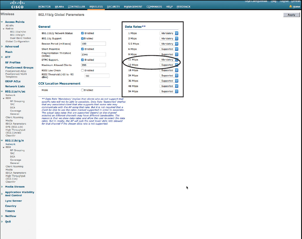
Note
Disabled rates are not supported by the AP, so the AP announces Basic or Mandatory rates that all clients must support in their drive, then Supported rates that clients may or may not support while still being allowed to join the cell. Today, all clients support all rates in their driver, but this feature is still a way to position a lower boundary to the cell, a distance beyond which messages cannot be demodulated, thus effectively reducing the efficiency footprint of the cell. Also, as per 802.11, multicast is always set at a Mandatory rate. Cisco APs send multicast at the highest mandatory rate supported by all intended recipients. Setting 24 Mbps as Mandatory allows the AP to switch to 24 Mbps if all recipients are close enough. By contrast, broadcasts are sent at the lowest mandatory rate.
These recommendations apply to the legacy rates (802.11b/g/a). For these rates, the Wi-Fi Alliance tests that rates set to Disabled on the AP are effectively not used by the clients of that AP. However, no such test exists for 802.11n or 802.11ac rates. As a result, disabling 802.11n or 802.11ac rates is not useful. (Clients would still use them; you would just prevent your AP from responding at a similar rate.) However, disabling low legacy rates is enough to limit the cell edge, because the AP sends beacons at the lowest mandatory rate. (Stations that stop hearing the AP beacons typically determine that the AP is out of range and roam.)
AVC Configuration
Another element of your QoS configuration includes Application Visibility and Control (AVC). AVC performs deep packet inspection (DPI) to recognize close to 1,400 different applications, including about 170 encrypted applications. AVC is therefore a central element of an end-to-end QoS strategy. AVC can run on multiple platforms (WLCs, routers, and so on). However, there is a CPU and memory load cost associated with application recognition. That cost may be negligible or heavy, depending on the application mix transiting through your systems. In the real world, you would carefully weigh that cost to decide the best locations to run DPI. You may decide to run AVC on all routers, supporting switches, and on your WLC and APs, or just at selected locations. Only testing could decide the impact of running AVC at a given device location. (None of this is a consideration for the CCIE lab, where you can expect only a few clients.)
On FlexConnect APs running in local switching mode, AVC runs at the AP. In that case, AVC is a subset of the full AVC. On local-mode APs and FlexConnect APs running in central switching mode, AVC runs at the WLC. The location of the AVC task has practical consequences on QoS. AVC allows you to rate-limit traffic, drop traffic, or change the QoS marking of target traffic. In this last case, you should keep in mind that the AVC task runs inside the WLC and before the QoS downstream profiling task, as illustrated in Figure 7-30.
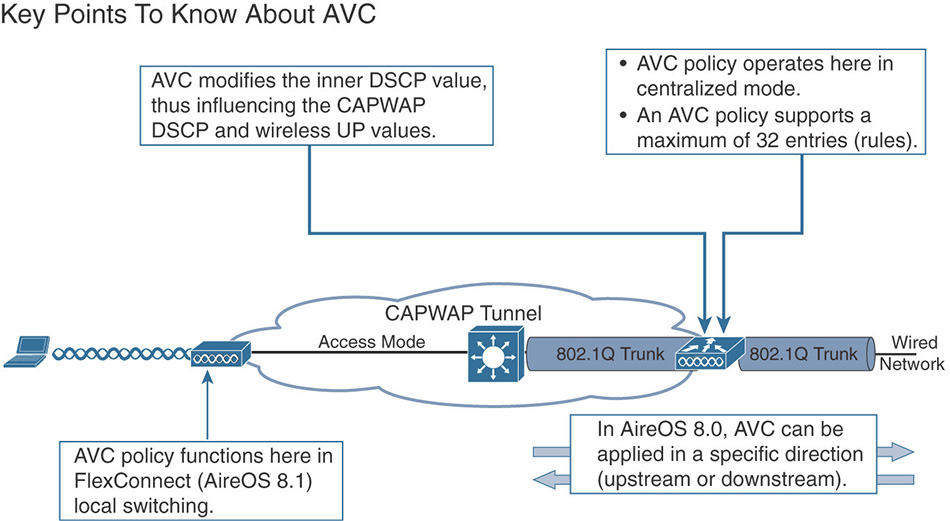
As an example, suppose that you receive a packet with DSCP CS3, and that your WLAN QoS profile is set to Gold (ceiling set to video, AF 41, UP 5). AVC runs first. Suppose that AVC recognizes that this traffic is in fact voice, and that your AVC policy dictates that this application should be marked EF (DSCP 46). AVC will perform this task first, remarking CS3 to EF, and will then pass the packet to the WLAN routine, where the QoS ceiling is examined. Because the new marking is above the ceiling, the CAPWAP outer header will be capped to AF41 (while the inner DSCP shows DSCP 46, as remarked by AVC).
The reverse logic can be seen upstream. Suppose that your WLAN ceiling is now Platinum (max DSCP 46, UP 6). A client sends DSCP 46 traffic upstream. This traffic will be forwarded to the WLC by the local AP. All along, the CAPWAP outer header shows DSCP 46, as you are within the ceiling limit. Yet, at the WLC, AVC determines that this traffic is in fact BitTorrent that should be remarked CS1. Traffic is remarked, then sent to the wire. The correct marking only occurred at the WLC, while the AP to WLC link was not affected.
These two cases are not gotchas that should be source of headaches for you. You should simply be aware of the way AVC works.
AVC for the WLC is configured in the GUI from Wireless > Application Visibility and Control > AVC Profile. Create a new profile, then edit the profile. You can then add rules that will target traffic and decide whether that target traffic should be marked, dropped, or rate limited, as shown in Figure 7-31 (CLI config avc profile).
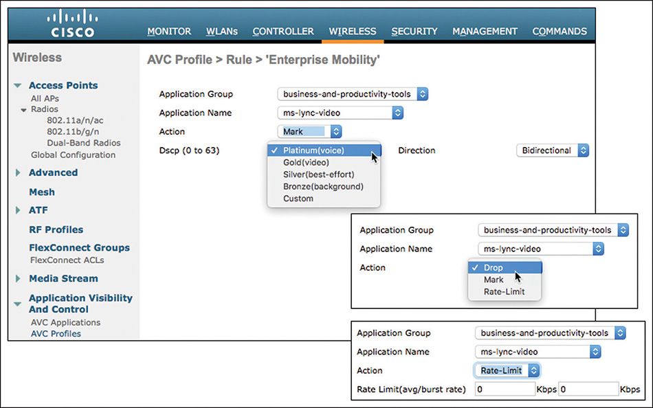
Dropping is a simple action, taken at the WLC for both upstream and downstream mode and local APs.
Rate limiting is also performed at the WLC (both for upstream and downstream) and adds to the other, more generic, bandwidth contract rules that you may have for the user or the WLAN. Two examples will make the logic clear. Suppose that your user has a general BW contract of 500 kbps and that HTTP traffic has a bandwidth contract of 50 kbps. Upstream, up to 550 kbps of traffic can come from this user. Inside the WLC, traffic will be examined, and any HTTP flow over 50 kbps (coming from that user or any other user) will be dropped. Downstream, incoming traffic will be examined, and any HTTP traffic in excess of 50 kbps will be dropped. Note that the bandwidth can be different for upstream and downstream.
Now suppose that your user has a general BW contract of 50 kbps and that HTTP traffic has a bandwidth contract of 500 kbps. That user can receive HTTP up to the user BW limit, 50 kbps, supposing that no other traffic for that user needs to share the bandwidth.
If you choose to remark, the AireOS 8.3 interface offers the interesting text “Dscp” but offers in fact one of the four Wi-Fi ACs. What is meant is that the remarking is static and will apply for both the DSCP and the UP value, based on the AC default values shown earlier in this chapter. The remarking can be bidirectional or applied only for downstream or upstream traffic. Figure 7-32 shows an example of AVC policy.
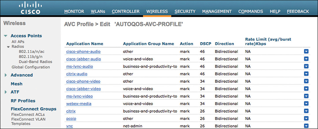
After you have created an AVC profile, you can enable AVC and apply the profile to a WLAN from the WLAN QoS tab (CLI config wlan avc). You can also apply a specific profile to class of devices (from Security > Local Policy > Edit Policy > Action, CLI config policy). The AVC profile can also be configured on the WLC, then called from within an Authorization profile on the AAA server with AAA override (see Figure 7-19 for an example of an Authorization profile).
Note
Only three applications can be rate limited on AireOS 8.3. You should not try to configure more than three rate limits.
AireOS supports only 32 applications per AVC profile.
If you configure AVC in a Foreign-Anchor scenario, you should configure the same policy on both sides. However, the key location where the policy will be enforced is the Anchor.
AVC for WLANs applied to FlexConnect APs in central switching mode follow the same rules as above. However, if you configure AVC for FlexConnect APs in local switching mode, the process is different. The flow is shown in Figure 7-33.
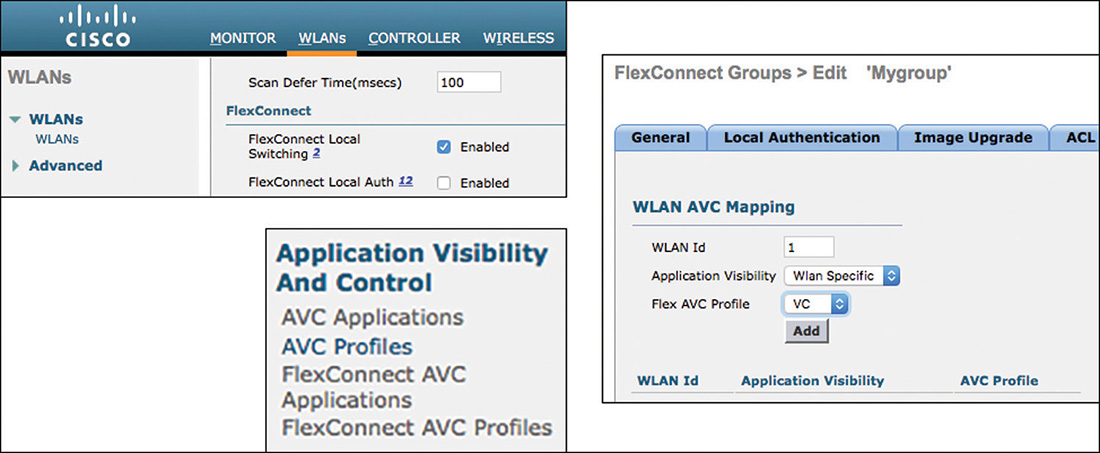
As soon as you enable FlexConnect Local switching on a WLAN, and plan to support AVC for FlexConnect on that WLAN, you need to configure a standard AVC profile for the Local Mode APs that will support it, and another AVC profile, from the Wireless > Application Visibility And Control > FlexConnect AVC Profiles submenu (CLI config flexconnect avc) for the APs in FlexConnect mode that will support this WLAN. The FlexConnect AVC profile uses a subset of the WLC AVC database with a different NBAR engine version, so you may not find the exact match to your Local mode AVC application.
After the profile is created, you need to apply it to the flexgroup to which the target FlexConnect APs belong, from Wireless > FlexConnect Groups > Edit > WLAN AVC mapping (CLI config flexconnect group <groupName> avc). In this screen, you can target specific WLANs and map a specific Flex AVC, or map a Flex AVC profile to all local switching WLANs supported by the APs in that FlexConnect group.
Note
AAA override for AVC is not supported for FlexConnect groups.
Configuring AVC enables you to monitor and control application traffic going through your system. You can view the application mix from the WLC GUI and CLI. However, there may be cases where you would want to export this view to another monitoring station. When Cisco Prime Infrastructure adds a WLC to its database, it also configures itself as a NetFlow destination. This allows you to monitor the WLC AVC traffic from the PI interface. If you want to export AVC data to other monitoring stations, configure a new NetFlow Exporter from Wireless > NetFlow > Exporter. The Exporter is the confusing way of saying “the server where you will send NetFlow data from this WLC.” Enter the target server name, IP address, and port (CLI config flow). Typically, NetFlow is sent to port 9995.
You can then configure the WLC to send data to this server. From Wireless >NetFlow > Monitor, create a new monitor profile. Click the profile and pick the server you want to send traffic to (it is likely to be the exporter you just created). You can choose to send None or Client App Record data (both options are acceptable, but read the question carefully, if you are in a lab environment). In all likelihood, you will want to send Client App Records.
You can then activate this profile on a per SSID-basis, from the WLAN > Edit > QoS tab. From the NetFlow Monitor drop-down list, choose the Monitor profile and click Apply (CLI config wlan flow <WLAN-ID> monitor <profile name> enable).
FastLane Configuration and Client Behavior
The strategy for your QoS configuration on AireOS depends a lot on what QoS features your clients support. In this field, there is a large variety of clients and behaviors, and feature scope changes fast. At the time of writing this book, clients could be separated into three categories:
Windows 7 and later devices: QoS can be pushed as a GPO policy; therefore, DSCP marking depends on the administrator’s QoS skills. However, these markings appear only as DSCP values. Microsoft has maintained the view that L2 marking should be the same, regardless of the medium type. As a result, the UP marking derived from the DSCP marking maps the 3 MSBs. With this scheme, voice is UP 5 and video UP 4, causing UP 6 and UP 7 to be unused, and causing voice and video to conflict with the 802.11 protocol and intent.
Android devices: These clients have an open operating system, which allows QoS marking support. However, marking depends on the app developer, the phone vendor, and the service provider. Both service provider and phone vendor may introduce OS modifications that could block app QoS marking. The purpose is generally to avoid QoS marking on devices that are intended to be low end. These devices are not expected on enterprise networks, and QoS is therefore not useful (in your home, competition with other traffic is limited). Additionally, some home service providers do not expect QoS traffic coming from home networks and either remark or drop QoS packets coming from home networks. This policy is old and is less frequent than it was in the years 2000s, but the side effect is still felt in the modifications made by some Android phone vendors. The consequence is that QoS marking is difficult to predict for Android devices. You may see UP and no DSCP, both DSCP and UP, or no QoS. Testing your network’s common devices is recommended. Also, keep in mind that the industry trends toward QoS adoption, and that new OS or vendor/SP software updates may unblock QoS marking in a phone that was only displaying best effort in the previous software version.
iOS and MacOS 10.13 and later: These devices support QoS as per best practices. Apple has been working with Cisco and the IETF for years. iOS 10 and Mac OS 10.13 adopt the QoS scheme shown in Figure 7-34.
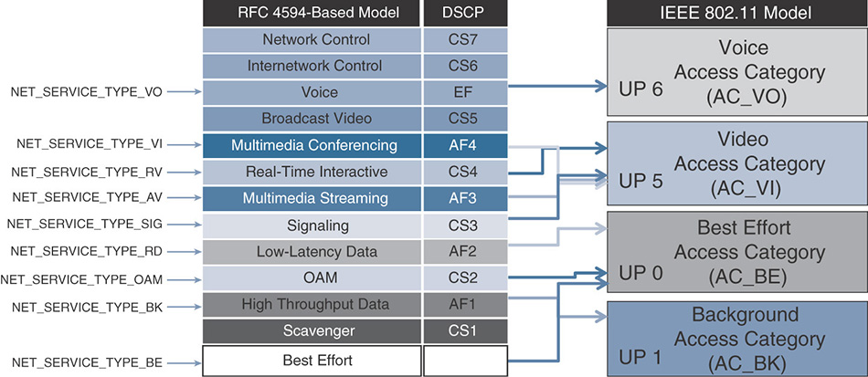
Figure 7-34 Apple iOS and MacOS QoS Sockets and Mapping
The operating system offers nine QoS classes available to app developers (as socket calls), and each class receives a DSCP marking that follows IETF RFCs (e.g., RFC 4594). Each DSCP translates to an UP marking that follows best practices, with a few minor exceptions. One exception worth noting is that Apple chose to limit the current span of the mapping logic to four ACs, but only one UP per AC, thus following the tradition of most other client and infrastructure vendors.
Cisco has worked extensively with Apple, also providing technical support to help app developers understand the differences between the various classes and choose the best class for each of their app calls. As a result, traffic coming from iOS (10 and above) and Mac OS (10.13 and above) applications is trusted. UP 6 traffic really represents voice traffic. As such, an exception was made in the ACM rules for iOS and Mac OS devices. You need to make sure that you understand this exception, because it applies on both sides. It starts from the fact that iOS and Mac OS devices recognize the signature present in Cisco AP beacons or probe responses. Similarly, the Cisco APs recognize Apple in the messages coming from iOS and Mac OS devices.
As a consequence of recognizing Cisco APs (and knowing that a trust relationship is formed), iOS and Mac OS devices ignore the ACM bit for UP 6 traffic. This means that these clients will send UP 6 traffic without TSPEC (iOS and Mac OS do not implement ADDTS/TSPEC), even if ACM is enabled for the voice queue in the SSID beacons. This is a vendor-to-vendor specific agreement. On other networks, iOS and Mac OS will revert to UP 5.
As a consequence of recognizing iOS and Mac OS, the Cisco AP honors the UP 6 traffic, even with ACM enabled and in the absence of ADDTS/TSPEC. As a result, traffic is forwarded as if ADDTS had happened and been successful. DSCP 46 is honored upstream and downstream, and DSCP 46 traffic is forwarded with UP 6 marking from the AP to the client.
Another particularity of iOS (10 and later) and Mac OS (10.13 and later) clients is their support of Fastlane. This feature is also the result of a partnership between Apple and Cisco. The logic of this joint development is that your network QoS configuration does not extend to the client device. Your AVC and QoS policies may start at the AP, extend to the entire network under your control, and also extend downstream to traffic sent to the client. However, you have no control over the client-to-AP traffic.
You also have no way to tell the client what your network QoS configuration looks like. This last element is important because each network has different requirements. For example, in a car dealership, a video game featuring the latest car may be business relevant (keep the customers happy while they wait), while the same car game may be seen as non-business relevant in a carpeted office. The network QoS configuration may be different, but the client is not aware of this difference.
To solve this issue, Apple leverages the Configuration Profile feature that has been present in iOS and Mac OS from the early days of the operating systems. The Configuration Profile defines parameters for your device (look and feel, security, and so on). Profiles have a Wi-Fi component that defines credentials and limitations for multiple SSIDs. Profiles are commonly leveraged by MDM (Mobile Device Management) solutions that create profiles for employees’ devices and deploy these profiles to the end devices based on the employee profile. This makes device management easier for large companies.
iOS 10 and Mac OS 10.13 allow a new component of the Wi-Fi section of the profile, called Restrict QoS marking. Figure 7-35 shows such a screen, using Apple Configurator. You can create such a profile in any tool that enables the creation of an iOS or a Mac OS profile. MDM solutions typically offer such an interface, but Apple Configurator is another solution as a program available on Mac OS.
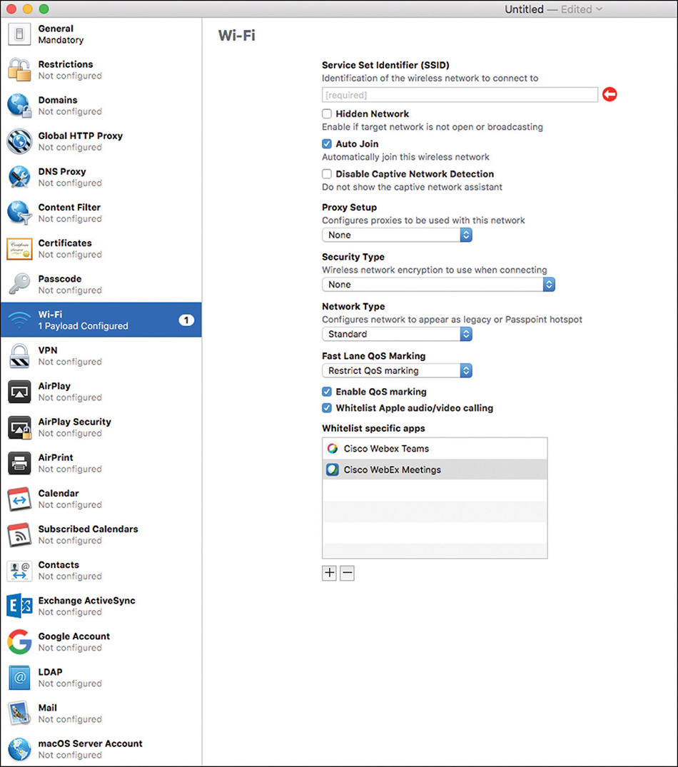
For each SSID, you can choose to control QoS marking. When this feature is selected, you can choose which applications should be in a whitelist (on Figure 7-35, applications are called by clicking the + sign; you then type the application name, and the tool retrieves the application identity details from the Apple applications databases in the cloud). Any application known to Apple can this way be added to the whitelist. Please note two important details:
The whitelist is created on a per-SSID basis. Two different SSIDs may have different whitelists, even on the same machine. This means that your iPhone policy may change as you change networks and location, based on the local network QoS policy requirements.
Facetime and Wi-Fi calling are special because they use the phone dialer. They are called Apple Audio/Video calling. Checking the associated check box puts these two applications in the whitelist, which is the default.
The profile is then installed on the Apple client device. Apple describes multiple ways of provisioning such a profile (MDM is one solution, but there are many others, such as web onboarding, emails, and the like). The expectation is that the policy installed on the client device, for a given SSID, matches the QoS policy configured on the infrastructure for that same SSID. This is an assumption, but by no means a guarantee. The client manager creates and pushes the device, while you configure the WLC QoS policy. Hopefully, you work with the device manager and with the Switch and Routing teams, so that the QoS policy is end to end, and everyone has the same understanding of what applications are business relevant and what classes of traffic are configured with what associated marking and QoS strategy.
On the wireless infrastructure side, you need to configure QoS in general. To support Fastlane, you also need to activate Fastlane in the SSID QoS tab, as shown in Figure 7-36.
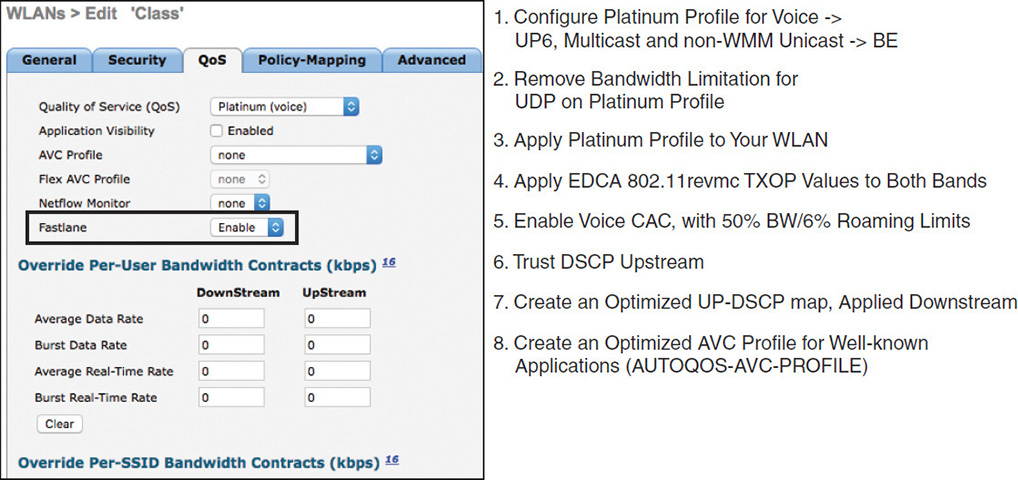
Enabling this feature has two effects:
In the exchanges with Apple devices, a special handshake allows Apple devices to recognize that Fastlane support is enabled on the SSID (the handshake format is proprietary).
Because enabling Fastlane indicates the will to support QoS, the Fastlane macro also configures your WLC for best practices, as shown in Figure 7-36. In short, all the best practices described in this chapter for QoS are configured. (The macro does not configure data rates, only QoS features.)
After the iOS or Mac OS client device gets in range of a Cisco AP Meraki or AireOS 8.3 and later, both sides recognize each other. At that time, the client checks whether there is a profile for that SSID, and whether the profile includes a whitelist component.
If there is no QoS component, all apps can mark QoS (as the developer configured them).
If there is a QoS component, only the apps in the whitelist are allowed to mark QoS. The apps that are not listed in the whitelist are considered nonbusiness relevant and will be sent without QoS marking (best effort). This allows the network QoS strategists to put in the whitelist the apps that are important for the local network and make sure that both the client and the network sides have the same understanding of which applications are business relevant, and QoS-worthy, and which are just personal applications that will receive best effort.
As a wireless expert, you should make sure that you understand Fastlane properly to face any question wording. This understanding includes dispelling silly rumors that you will read here and there.
Fastlane does not define the app QoS marking on the client device. All Fastlane does is define which apps are in the whitelist and which are not. Apps in the whitelist will use whichever QoS marking their developer designed for each socket call type. The fact that Cisco worked with Apple to define which type of traffic should get what type of marking as per IETF recommendations is only indirectly related to Fastlane and does not result in your AP sending QoS marking values to the client for app calls.
Apps that are not in the whitelist are separated into two categories. Most apps have been developed with best effort or higher marking (or no QoS). These applications are then sent by the client in the best effort queue. However, some apps have been developed to send traffic as background (for example, backups and other slow file uploads). Because these were already set to use a lower priority queue, Fastlane keeps them in the background. In other words, these applications do not get promoted to best effort, they stay background, regardless of their position within the whitelist.
If Fastlane is not enabled in the WLAN, or if you are in a non-Cisco network, the apps mark only UP, but DSCP stays at CS0 for all applications (regardless of your whitelist configuration). The reason is that in such configuration, the network is not seen as end-to-end QoS enabled (it could be your home), and QoS is not deemed as important beyond the wireless link.
In AireOS, enabling Fastlane on any WLAN creates an AUTOQOS-AVC-PROFILE that contains the 32 most common network applications and their recommended QoS markings. However, Fastlane does not activate Application Visibility on the WLAN. The profile is created in the background, ready to be used.
If you activate AVC on a Fastlane-enabled WLAN, AUTOQOS-AVC-PROFILE is the only AVC profile that you can use on AireOS 8.3. AireOS 8.4 removes this limitation. In any AireOS version where this AUTOQOS-AVC-PROFILE is created, you can edit the profile, change the marking for any application, and remove any application to add another one instead. Although AireOS 8.3 mandates that you use this auto profile, you can customize the profile.
Be careful: In some AireOS 8.3 releases, the AUTOQOS-AVC-PROFILE is created every time you activate Fastlane on a WLAN. If you need to modify the auto profile, make sure to do so only after activating Fastlane on all WLANs where you need it.
Fastlane also configures the WLC for QoS best practices. You can individually edit and change any of these configurations. Fastlane is a simple macro.
When you disable Fastlane on a WLAN, the WLAN is returned to the default states, not the previous states. In other words, when you create a WLAN, the default QoS policy is Silver. If you change the QoS policy to Gold, and then enable Fastlane, the WLAN QOS policy changes to Platinum. If you then disable Fastlane, the WLAN QoS policy returns to Silver (the default).
The same default logic applies to any other QoS feature. When you remove Fastlane from a WLAN but other WLANs have Fastlane configured on the same WLC, only the target WLAN returns to its defaults. However, when you disable Fastlane on the last WLAN where Fastlane is enabled, the WLC QoS configuration returns to its defaults. For example, CAC is disabled and the Max RF Bandwidth value is reverted to 75%; the Unicast Default Priority and Multicast Default Priority in the Platinum profile are returned to their defaults, voice.
Enhanced Roaming
Fastlane is often associated with another feature jointly supported by Apple and Cisco, this time solely for iOS devices: enhanced roaming.
Enhanced roaming is only indirectly related to QoS and is about faster roaming. In this context, two elements appear:
802.11k and 802.11v are enabled by default on any new WLAN. iOS devices support these two protocols in the same way that Cisco implemented them. 802.11k provides a list of the closest neighboring APs (up to 6) to the client joining the cell. This allows the client to have a shortlist of channels to scan (up to 6, instead of more than 20) when later getting close to the edge of the cell. 802.11v allows for a directed exchange when a client gets to the edge of the cell and is in urgent need of a candidate channel and AP to roam to. The AP can provide such next-best AP information based on the client location. Figure 7-37 contrasts 802.11k and 802.11v.
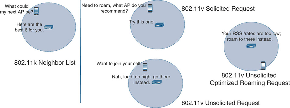
Figure 7-37 802.11k Versus 802.11v A new mode, Adaptive 802.11r, is created. iOS clients support 802.11r, an amendment facilitating the fast exchange of WPA2 keying material during roaming events. However, many networks do not implement 802.11r (even in combination with standard WPA2) because some old clients, incompatible with 802.11r, may fail to associate if 802.11r is mentioned in the WLAN parameters (even if, in hybrid mode, the client can use either 802.11r or regular WPA2). As a consequence, a useful feature is widely underdeployed. Adaptive 11r leverages the secret handshake that iOS and Cisco APs run, recognizing each other, to dynamically enable 802.11r for individual iOS (iOS 10 and later) clients, while support for 802.11r is not advertised in the cell.
Note
Adaptive 802.11r is the default security mechanism for new WLANs in AireOS 8.3 and later. It is considered a best practice, unless you do not have any iOS clients in your network or unless you enable 802.11r openly in the WLAN.
802.11k and 802.11v do not require specific configuration, because both are enabled by default in the Advanced tab of the new WLANs you create in 8.3 and later, as shown in Figure 7-38.
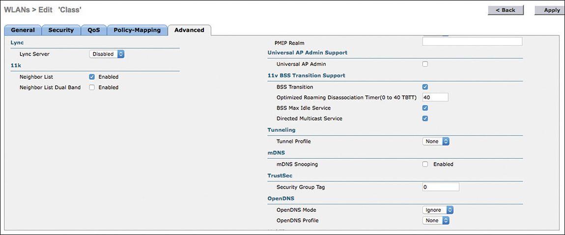
However, you should be aware of the available options.
802.11k is enabled by checking the Neighbor List check box. This box should be checked by default on new WLANs.
802.11k includes several modes. The mode activated by the Neighbor list option (and on iOS devices) is the AP neighbor report. The client associates to the WLAN, and right after association sends an Action frame of Category Radio Measurement, with a Neighbor Report Request. The AP responds with another Action frame in the Radio Measurement family, which type is Neighbor Report Response, as shown in Figure 7-39. 802.11k also allows the AP to ask the station for similar reports, but that mode is not implemented in 8.3 or iOS. Also, the neighbor report could be asked at any time, but iOS asks for the report only at association time. Other vendors also support 802.11k and may make the request at other times (for example, some Intel enterprise chipsets make the request when the AP RSSI falls below a target threshold). There is not really a mode that is better than the other; the neighborhood is unlikely to dramatically change between the time the client associates and the time the client needs to roam away.
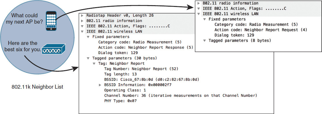
By default, the Neighbor List includes neighboring APs and channel information only for the client current band, which is best practice. You can check the Neighbor List Dual Band option to also send information about neighbor information in the other band (for example, 2.4 GHz radios for a client currently associated to a 5 GHz radio). Keep in mind that 5 GHz is usually considered better than 2.4 GHz. In most cases, the cell coverage in 5 GHz should be sufficient to maintain the client in that band across the entire floor, and iOS clients prefer the 5 GHz band anyway (this band is scanned first, and preferred if at least one of the discovered APs signal in that band is above −65 dBm). Therefore, single-band (with the expectation of that band being 5 GHz) messaging is preferred over dual-band messaging.
AireOS 8.3 also includes an Assisted Roaming Prediction Optimization option. This option is for non-802.11k clients. Its logic is to construct the same neighbor list that 802.11k would build (best neighboring APs) and force non-802.11k clients to prefer these neighbors. When the non-802.11k client associates, a neighbor list is generated based on the client pre-association probes (which APs heard the client best) and stored in the mobile station software data structure. Clients at different locations have different lists because the client probes are seen with different RSSI values by different neighbors. Because clients usually probe before any association or reassociation, this list is constructed with the most updated probe data and predicts the next AP that the client is likely to roam to. Then, when the client roams, association is denied to the APs not in that neighbor list. This mode is a bit aggressive, because the client does not know the neighbor list. Therefore, it may have undesirable side effects (such as the client temporarily dropping off Wi-Fi because the client is denied on several APs). This option is in fact removed from the GUI (CLI only) in later AireOS codes to avoid “let’s check everything on that page” syndromes. Enable it carefully. Most of the time, keeping it disabled is better for real-time applications (let the client roam where it needs). If you enable it, you can also tune the assisted roaming options (these only apply to non-802.11k assisted roaming, not to 802.11k):
Denial count: Maximum number of times a client is refused association.
Prediction threshold: Minimum number of entries required in the prediction list for the assisted roaming feature to be activated.
802.11v is activated by checking the BSS Transition option (should be enabled by default on new WLANs).
In the 802.11v Solicited Request and 802.11v Unsolicited Optimized Roaming Request modes, the AP suggests a better AP to an associated client. At that time, the AP can even be more directive, and say “go to that AP, AND if you are not gone after delay X, I ‘may’ disconnect you” (disassociation imminent bit). This bit is set if you check the Disassociation Imminent check box. The delay is also advertised in the 802.11v message and configured in the Disassociation Timer field. Note that the time unit is TBTT (Target Beacon Transmission Time), or beacon intervals.
The AP will not in fact disconnect the client unless you also configure Aggressive Load Balancing (which needs to be enabled at the WLAN level in the Advanced tab, and can be edited in Wireless > Advanced > RF Management > Load Balancing). Aggressive Load Balancing is not recommended for networks with real-time applications. In these networks, you want to let your client roam fast, even if the next AP is not the best, rather than be picky and force the client to drop voice packets while you try to convince it to get to a better AP.
You can also disconnect the client after a number of TBTTs when also configuring Optimized Roaming (in Wireless > Advanced > RF Management > Optimized Roaming). In that case, the Optimized Roaming Disassociation Timer at the WLAN level will be used.
Note
Aggressive load balancing works based on the client probes, denying the client association requests to APs that are not “the best” for that client.
Optimized roaming works based on signals, sending a deauthentication message to associated clients when these clients’ signal fall below a configurable threshold. The expectation is that the disconnected client will then try a better AP.
In the 802.11v section of the Advanced tab, you will see two items unrelated to roaming but related to 802.11v. (802.11v is a 400-page long amendment, with multiple features around network management to make the life of clients in the cell better.)
BSS Max Idle Service allows the AP to send to the client the idle timeout for the cell. This timeout is about idle (sleeping) clients that do not send or receive traffic for a while. All cells have one, and this is the interval beyond which the AP will consider that a silent client is in fact gone (and the AP will remove the client from the list of active clients in the cell). The client will have to start from scratch (authentication request, and so on) to rejoin the cell. Strangely enough, 802.11 did not have a way for the AP to communicate that timer to its clients before 802.11v, forcing the clients to wake up often and send a frame (even a null frame) to tell the AP about their presence in the cell. With the BSS Max Idle Service, the AP tells the clients about the idle timeout. Clients supporting this feature (for example, iOS clients) can then sleep for a longer time and stay passive or silent for up to that idle timeout period without being removed from the cell.
An effect of the BSS Max Idle Service is that the client may sleep for more than one beacon interval, and more than one DTIM interval. (Recall from your CCNA that the DTIM is the beacon interval at which the AP will send broadcasts and multicast messages to the cell. Clients should wake up at each DTIM to get those messages. If they sleep beyond a DTIM, they may miss broadcasts or multicasts messages.)
In that case, the AP can advertise the Directed Multicast Service (DMS) option, allowing clients to register for specific flows. When DMS is activated, a client going to sleep can request the AP to keep target multicast or broadcast traffic (for example, “Please keep for me any multicast message sent to 224.0.0.251 while I sleep”). The AP will send the broadcast or multicast message for the other clients at the DTIM interval, but will also keep a copy. When the client wakes up (any frame from the client where the Power Management bit is set to 0), the AP will unicast to the client a copy of the saved multicast/broadcast messages. iOS devices support both BSS Max Idle Service and DMS, and these options are enabled by default. Keeping them enabled is best practice, because they improve the life of supporting devices in the cell and do not impact the others.
Adaptive 802.11r is the default security mode on new WLANs in AireOS 8.3 and later. Adaptive 802.11r is one of three fast roaming (Fast Transition, FT) options:
Adaptive 802.11r (Fast Transition set to Adaptive, as shown in Figure 7-40): 802.11r (FT) is not advertised in beacons and probe responses. iOS devices are recognized (and they recognize Cisco WLANs); FT is enabled individually for these devices when they associate.
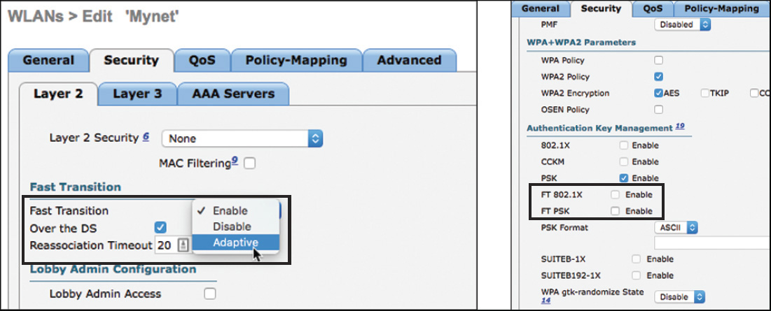
Figure 7-40 Adaptive 802.11r Configuration Fast Transition Disable: 802.11r is disabled, not advertised, and not enabled, for any client.
Fast Transition Enable: FT is enabled and advertised in beacons and probe responses.
If you enable FT for your WLAN, you can choose a strict 802.11r key management mode, or a hybrid mode:
If you set FT to Enable and choose key management to be either FT PSK or FT 802.1X, the WLAN is strictly FT. Only 802.11r-compliant clients can associate to the cell.
If you set FT to Enable and choose key management to be a combination of FT and non-FT, choosing either FT PSK and PSK, or FT 802.1X and 802.1X, the WLAN is hybrid. Both 802.11r and WPA2 are advertised in the beacons and probe responses. 802.11r clients are expected to associate using 802.11r, whereas non-802.11r clients “should” associate using standard WPA2.
If you set Fast Transition to Adaptive, your key management must be either 802.1X or PSK (CCKM is a neutral option; you can enable it or not), as shown in Figure 7-40.
You should not enable any FT key management option. If you enable an 802.11r key management option (FT PSK or FT 802.1X alone, or the hybrid combination FT PSK/PSK or FT 802.1X/802.1X), you enable 802.11r openly. As a result, 802.11r is advertised in your SSID beacons. This contradicts the purpose of Adaptive 802.11r, because Adaptive 802.11r is designed for networks where you do not want to, or cannot, advertise 802.11r openly. Enabling Adaptive 802.11r in a network where 802.11r is advertised openly does not make sense. If 802.11r is advertised openly, the iOS devices will use it directly, no need for any adaptive mode or secret handshake.
Note
Not all iOS devices support Adaptive 802.11r. iPhones 6S and later and iPad Pros support 802.11r, but older devices do not.
Managing Video Flows
Video conferencing falls into the realm of real-time applications, and the recommendations in the previous section apply. However, you may have other type of video traffic in the Multimedia Streaming category (for example, your beloved CEO daily broadcast). In many networks, this one-way flow is sent over multicast. Multicast is great for wired networks but has a major drawback for Wi-Fi networks: it is sent per 802.11 requirements at one of the Basic (mandatory) rates. Only legacy rates (802.11, 802.11b, 802.11g, or 802.11a) can be set to Basic. The result is that these multicast flows will be sent at a suboptimal rate (instead of 802.11n or 802.11ac wherever possible).
In most networks, you would set 12 Mbps and 24 Mbps as mandatory rates, and multicast flows will be sent at the highest mandatory rate supported by all receiving stations. In an 802.11n or 802.11ac network, it is far more efficient to send 10 individual frames at 300 Mbps than a single multicast frame at 24 Mbps (that all stations in the cell will receive, because the destination address is multicast, even if they do not need it).
To work around this issue, you can configure media streams, also called VideoStreams. With media streams, the WLC will keep track of wireless clients subscribing to targeted multicast flows using IGMP membership reports. When such messages are transmitted by wireless clients, the WLC will record the flow address that the client is subscribing to. Then, when such flows will be forwarded to the client through the WLC, the WLC will unicast the flow to the client. This is the general principle; the flow details are as follows:
Note
Please note that this section focuses on video flows, but media streams are in fact about multicast streams, regardless of the payload they carry. You can configure media stream even if your multicast flow carries something else than video, like multicast paging messages for voice badges for example, or any other multicast traffic where there is a subscription mechanism for the clients.
The WLC intercepts the IGMP reports from each multicast client.
The WLC sends a Radio Resource Control (RRC) request to the AP. This request aims at checking whether there is enough space for a unicast stream in that cell. This verification acts as a filter, which allows you to decide which flows should be forwarded to the cell if the channel utilization is high (and which flows are of lesser importance and should be dropped or sent as best effort).
The AP returns an RRC response for the client and the radio, providing a view of the channel utilization.
The WLC determines whether the media stream flow that the client requested can be admitted for that AP and that radio.
The WLC creates a new multicast group ID (MGID) if the request flow is new, or adds the client to an existing MGID if other clients on that same WLC have already subscribed to that same multicast flow.
The WLC forwards the client join report upstream (to the wire).
If RRC revealed that enough bandwidth was available, the WLC informs the AP that the stream is admitted and that bandwidth must be reserved.
The WLC also sends to the AP the MGID and WLAN mapping.
The AP keeps track of MGID, WLAN, and client association.
Then, when multicast traffic flows from the source toward the client:
The WLC checks whether media stream was set with RRC for that flow.
If media stream was not configured for that flow, the flow is dropped or sent as best effort, depending on configuration.
If a media stream exists, the WLC forwards to all APs allowing that flow, using Unicast or Multicast.
DSCP AF41 is used by default for the CAPWAP outer header by default. Traffic is sent without DTLS encryption if multicast is used between the WLC and the APs (even if you checked the data encryption option in the AP Advanced tab; encryption is used if you use unicast between the WLC and the APs).
The AP changes the Layer 2 destination address to unicast and forwards to each client.
Sent at optimal rate for each client, WMM Video (AC_VI) queue.
This choreography means that your WLC must not only be configured for media streams but also for multicast.
The first item to configure is the WLC to AP traffic mode for multicast. This mode determines whether a multicast flow received by the WLC should be sent individually to each AP or if it should be sent once to a multicast address to which the APs subscribe.
Note
Don’t fall into the traps around this point. If your WLC is receiving multicast traffic destined for wireless clients, it is likely that your wired infrastructure supports multicast (otherwise that multicast traffic would not have reached the WLC). Therefore, it may be beneficial to leverage this infrastructure multicast support. If the WLC has a message that needs to be sent to all APs, it is more economical to send one multicast message to an address to which all APs subscribe rather than sending a unicast message to each AP. The APs joining the WLC will get in their config this multicast address membership and will send IGMP membership reports for that address, letting the wired multicast infrastructure know that packets sent to that multicast address should be forwarded to each subscribed AP. As a result, the WLC sends one message to a multicast address, and that message is forwarded to each subnet where there are APs. This is better than sending 1000 unicast messages (if the WLC has 1000 APs).
However, the AP Multicast mode has nothing to do with the multicast messages sent to the wireless clients. There is a reasoning that if the WLC receives multicast traffic for the wireless clients, then the infrastructure supports multicast, so why not leverage this fact for the WLC to AP forwarding part.
In Controller > General, you can set the AP multicast mode to unicast or multicast:
With unicast multicast mode, each multicast packet received by the WLC for wireless clients will be encapsulated into a unicast packet and sent to each AP individually. If you have 1000 APs, the WLC sends 1000 messages (regardless of which AP has clients for this traffic).
With multicast multicast mode, each multicast packet received by the WLC for wireless clients will be encapsulated into another multicast packet and sent once to the wire. As the APs subscribe to that outer multicast address, the multicast infrastructure will forward that one packet to each segment where there is a subscribed AP, and all APs will receive the packet. If you choose multicast multicast mode, configure a multicast address for your APs.
Note
The multicast multicast address has nothing to do with the multicast packet sent for your wireless clients. It is the common address that the APs subscribe to. An address in the multicast Organization Local Scope range (any address between 239.0.0.0 and 239.255.255.255) is a reasonable choice for IPv4 and, for example, the equivalent in IPv6 (ff1e::239.x.x.x).
Suppose that your multicast multicast address is 239.1.1.1, and suppose that your WLC receives traffic sent to the mDNS/Bonjour address 224.0.0.251. The WLC will convert the 802.3 frame into 802.11 (the destination IP is still 224.0.0.251), then encapsulate that frame into a CAPWAP packet. The CAPWAP outer header destination IP will be 239.1.1.1 (the source will be your WLC management interface IP address). The multicast infrastructure will forward the packet to all segments where clients are subscribed to the 239.1.1.1 address (that is, all the APs on that WLC).
Each AP will receive the multicast CAPWAP packet, will remove the CAPWAP header, look at the internal destination IP address (224.0.0.251), check which radios and SSIDs have clients for that flow (clients that subscribed to 224.0.0.251 flow), and will either forward the 802.11 frame to each matching SSID and radio or drop the packet if no client was found for that 224.0.0.251 address. (If IGMP/MLD snooping are disabled—see below for more details on snooping—then all the APs will transmit the original 224.0.0.251 multicast packet over the air, even if no clients are interested in this multicast service. This is obviously less efficient and consumes airtime in vain.)
The AP multicast mode configuration is only about WLC-to-AP traffic and is irrelevant for your client multicast forwarding (you can forward multicast traffic to clients with AP unicast mode or multicast mode).
If you want to allow multicast traffic to be forwarded to wireless clients, you need to go to Controller > Multicast and enable Global Multicast Mode, as shown in Figure 7-41 (CLI family config network multicast).
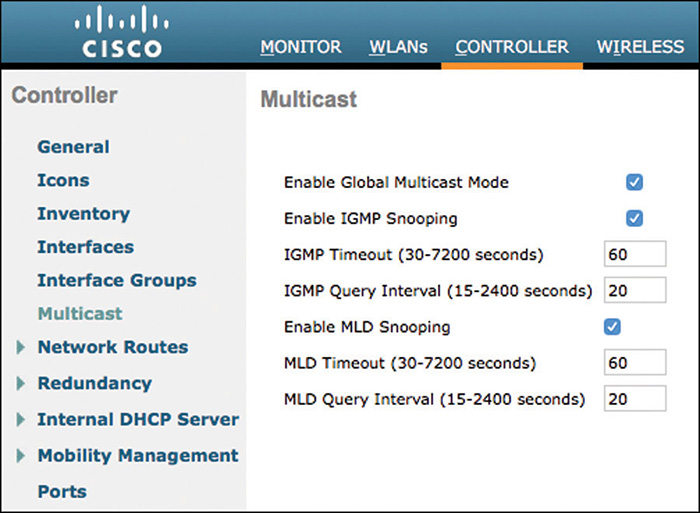
When Global Multicast Mode is disabled, incoming multicast traffic is not forwarded to clients and is dropped at the WLC. Clients may try to subscribe to multicast flows by sending IGMP membership reports, but the WLC will also drop these messages.
After Global Multicast Mode is enabled, multicast traffic can be forwarded to clients. The WLC can then also forward the client’s membership reports to the wired infrastructure. Two modes are possible:
Without IGMP (IPv4) or MLD (IPv6) snooping, the WLC forwards each membership report message to the wired infrastructure. This mode is chatty. If 500 clients subscribe to the same flow within a minute, the WLC will transparently relay each of these 500 messages upstream. The upstream infrastructure directly sees the clients as the requesters (called the multicast listeners).
With IGMP (IPv4) or MLD (IPv6) snooping, the WLC acts as a buffer. The WLC receives all the membership reports from the wireless clients but only forwards upstream one membership report per multicast address, at regular intervals. The upstream infrastructure does not see the clients, but the WLC as the multicast listener.
Each client will maintain its membership for each multicast address by sending membership reports at regular intervals. The interval is often semi-random (within a range) to avoid collisions between members’ packets. The WLC keeps track of these reports and associates each client and each multicast address to a multicast group identifier (MGID).
At regular intervals (configured with IGMP Query interval for IPv4 and MLD query interval for IPv6), the WLC will query the wireless clients for membership, to verify which clients still want to belong to which MGID. Default values for these queries (20 seconds) is fine in most cases. The IGMP query will be sent to all APs (unicast or multicast), then forwarded to all radios/SSIDs where multicast clients are reported.
Each client should respond to the query. If a client does not respond for a specific group for more than the interval configured in IGMP timeout (IPv4) or MLD timeout (IPv6), that client is removed from the matching MGID. Default values for this timeout function are fine in most cases. When the last client is removed from an MGID, the WLC stops forwarding upstream membership reports for that multicast address.
Enabling Global Multicast Mode on the WLC allows the WLC to forward multicast traffic to the wireless clients. You then need to decide whether that traffic should be sent over the air to all requesting clients as a slow common multicast packet or as faster individual unicast packets. Default is multicast. If you want to send unicast frames, navigate to Wireless > Media Stream > Streams (CLI config media-stream) and add a new stream as shown in Figure 7-42.
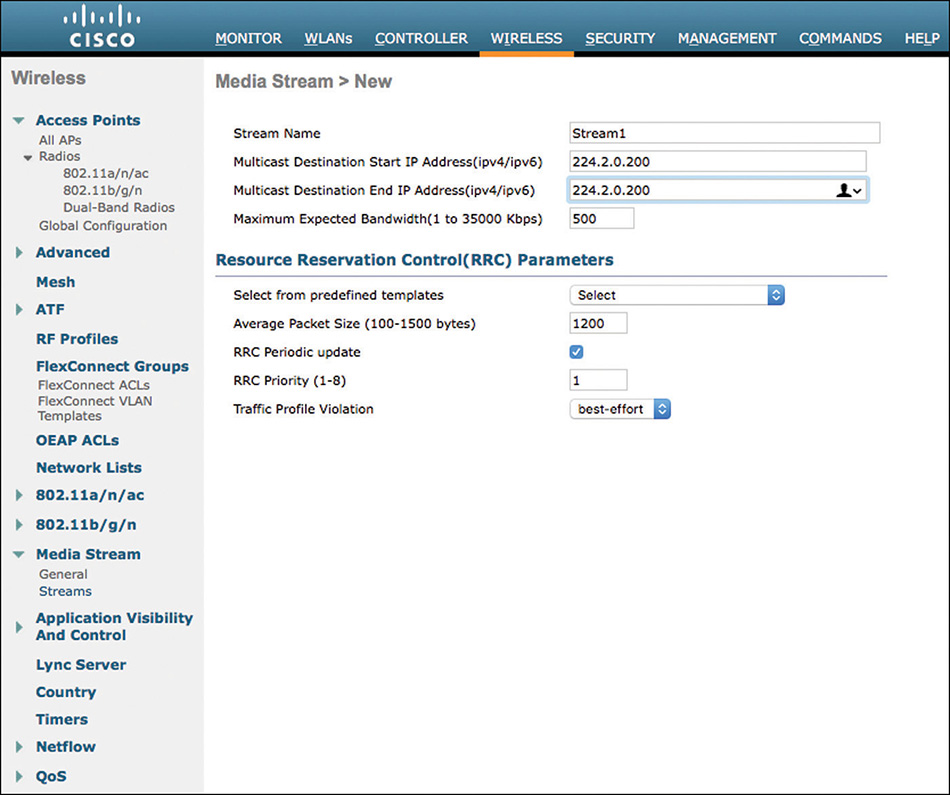
Most streams are sent to a single IP address, but some streams are sent to a range of addresses. Enter the range or the IP addresses in the Multicast Destination Start IP Address and Multicast Destination End IP Address fields. You also need to know the expected multicast stream bandwidth consumption. In the real world, this information should be provided by the flow emitter (based on the codec used for the video flow, for example). You can also measure the consumed bandwidth if needed.
The bandwidth is useful for RRC, to determine how much bandwidth should be reserved. However, video is bursty, so you may have periods of heavy traffic followed by quieter periods (different flow characteristics all resulting in the same average bandwidth). In the RRC section, you can use a predetermined template or define yourself the expected average packet size. In most cases, using a template is easier if you are not sure about the right values.
You can also decide whether RRC should be refreshed periodically to reevaluate the bandwidth available on the AP radio at regular intervals. This periodic reevaluation is the recommended setting, especially if you expect the channel utilization to reach critical levels or if you allow several multicast flows to your cell.
You can then specify the priority of this media stream. The priority can be any number between 1 and 8. A larger value means a higher priority. The default priority is 4. The low priority stream may be denied in the RRC periodic update, if there is not enough bandwidth for all streams on a given AP radio.
This “not enough bandwidth for all” condition forces the WLC to send first the flows with higher priority, then decide what to do with the flows of lower priority. This is the Traffic Profile Violation value. It specifies the action to perform in case of a violation after a re-RRC (not enough space, and this stream is not among those of higher priority; sending it would bring the AP radio to go beyond a utilization threshold that you will configure in the next page). Choose an action from the drop-down list. You can choose to drop the stream or to fallback, which means that the stream will be sent but demoted to best effort (instead of AF 41).
This way, you can create several media streams.
Creating these streams will allow you to send them as unicast wireless frames whenever possible. However, creating the stream alone does not enable this type of forwarding. You also need two additional steps: enabling media stream in general, and enabling media stream for your target WLANs.
In Wireless > Media Stream > General, check the Multicast Direct feature check box. This check box acts as a general on/off switch for multicast direct. Lower in the page, you can choose to enable Session Announcement State. This feature is useful in theory, to send messages to multicast receivers when their stream has to be stopped. This happens after a RRC reevaluation for streams of lower priority that have to be dropped because they consume too much bandwidth. The Session Announcement State allows you to send a note (for example, “Dear user, your video does not matter to the business, we dropped it. Sorry, now go back to work”), along with a phone number, email address, or URL that the user can reach to get more information (or complain).
After the Multicast Direct feature has been enabled, you can also activate multicast direct on the SSIDs where you would want multicast streams to be sent as unicast frames. This is done with the CLI config wlan media-stream multicast-direct <WLAN ID> command.
At this point, you are allowing media stream unicast in general and for selected WLANs, but you are not controlling the maximum bandwidth yet (the threshold that will help RRC determine when to deny or accept a flow). This is done from Wireless > 802.11a/n/ac | 802.11b/g/n > Media > Media. In this page, you can enable or disable bandwidth monitoring and control for media stream with the Unicast Video Redirect check box (CLI config 802.11a media-stream video-redirect). When this feature is enabled, you can also control how much bandwidth should be used on each radio for all media traffic with the Maximum Media Bandwidth option (CLI config 802.11a media-stream multicast-direct family).
Note
Be careful, this field represents the maximum bandwidth for media that is video traffic. Maximum is 85%. However, the bandwidth allocated for all types of media traffic also cannot exceed 85%. This total also includes the voice bandwidth. This has two consequences:
If you configure 50% bandwidth for Voice CAC and 65% for maximum media bandwidth, you are telling the system that it should stop admitting TSPEC voice calls when voice calls represent 50% of the bandwidth on the radio. But you are also saying that RRC should start dropping (or sending as best effort) multicast flows representing more than 65% of the bandwidth. The system will check each parameter individually. Because your total is more than 85% (it is actually more than 100%), you may face cases where media streams and voice suffer from poor quality. As much as possible, make sure that Maximum Media Bandwidth and Voice CAC Max RF Bandwidth (when configured) do not exceed 85%.
As you will see in the next section, you can also configure Video CAC. Voice CAC bandwidth and Video CAC bandwidth together cannot exceed 85%. (The system throws an error if your configuration exceeds this threshold.) You can consider the video admitted under Video CAC as part of your multicast media flow, if that video is sent over multicast. In that case, it does not make sense to have Video CAC different from Maximum Media Bandwidth. However, CAC video can also be unicast. In this case, the numbers in Video CAC bandwidth and Maximum Media Bandwidth are unrelated.
Sending unicast frames to an 802.11n/ac client is likely to be efficient. However, if the client is at the cell edge at 6 Mbps, one multicast packet is likely better than many unicast slow packets. Therefore, you can also configure the minimum PHY rate at which each multicast client should be for the system to attempt unicast transmission instead of multicast (CLI config 802.11a cac media-stream multicast-direct min-client-rate).
Efficiency (that is, speed of transmission) is one parameter. However, another advantage of unicast frames is that they are acknowledged. This is a reason why you may want to keep the client PHY rate to 6 Mbps, to increase the transmission quality (by resending frames that were not acknowledged). When the client is at the edge of the cell or in poor RF conditions, this requirement to use unicast may result in high retry rates. You can configure the maximum retry percentage of the transmissions. Beyond the configured number, the AP drops the frames when they are not acknowledged and sends the next ones (restarting to retry whenever needed, when the retry rate falls back below the threshold).
Lower down in the page, you can also configure how many streams should be allowed per AP radio and per client. You can also configure whether flows in excess of the configured bandwidth should be dropped or sent as best effort. These parameters are activated together with the Multicast Direct Enable option (CLI config 802.11a media-stream multicast-direct).
You can optionally configure Video CAC from the Video tab. The logic here is similar to the Voice CAC detailed earlier in this chapter, with a few additional considerations:
The bandwidth for Voice CAC and Video CAC together cannot exceed 85%.
You do not have to configure Video CAC for configuring Media Stream. It is an optional addition, even if it appears in all media stream configuration guides. In the exam, double check to verify whether this element is requested.
In real life, no client (at the time of publication) supports Video CAC; therefore, this feature is not useful.
Bonjour/mDNS
If you use Apple iOS or macOS devices, you also have to manage another type of traffic, Bonjour. In most cases, this traffic will not represent a large volume, but its structure has consequences on your network efficiency.
Bonjour/mDNS Principles
Apple Bonjour is part of the larger multicast DNS (mDNS) family. Subscription and traffic for this protocol are sent to the IPv4 address 224.0.0.251 and IPv6 address FF02::FB. These addresses are part of the nonroutable family. They are well suited in a small home network where the Bonjour traffic is expected to stay in the local subnet; however, this nonroutability is an issue for enterprise networks. The WLC has multiple functions to help Bonjour traffic delivery, beyond simple multicast forwarding. (Multicast forwarding may address the issue of letting clients receive Bonjour traffic, but does not address the issue of Bonjour devices in different subnets needed to communicate, and it is less efficient because it forwards all mDNS traffic without filtering for specific services, or VLAN, or WLAN, or other options as you will see later.)
mDNS gateway: The WLC can act as a proxy to let mDNS wireless devices communicate with mDNS devices in other subnets (whether they are wireless or wired).
mDNS policing: The WLC can generate conditions for this communication, based on group membership, profiles, or other criteria.
mDNS AP: An AP can report to the WLC the mDNS traffic heard on the AP switch. This is useful, for example, in classrooms, where the mDNS wired devices are close to the AP (and the students) but far from the WLC (the WLC is in another building and another VLAN, and would have no knowledge of these remote wired mDNS flows).
Location Specific Services (LSS): Wireless mDNS queries and advertisements are tagged with the AP MAC. Exchanges are allowed only for devices that have the same AP MAC tag (clients of the same AP, regardless of the band or the SSID) and devices on neighboring APs (devices for which the AP MAC tag match APs in the local AP AP-NEIGHBOR-LIST in the WLC RRM database, and that therefore are in the same RF neighborhood as the local AP). Note that this tagging does not apply to wired messages, only to wireless messages. (Wired messages are considered non-location-specific and are forwarded to all when allowed.)
Origin Based Service Discovery: This feature allows the WLC to tag an mDNS service to specify whether it comes from a wired or a wireless source. You can then decide to allow only wired or wireless services. Again, LSS would apply only to wireless services. You can use Origin Based Service Discovery to admit only wired mDNS, but you cannot add LSS in that case.
Priority MAC: To avoid overloading of the WLC mDNS database, you can configure up to 50 MAC addresses (each corresponding to a MAC address and an mDNS service) that are always on top and always discovered (if present). This is useful if you have a large number of mDNS devices advertising multiple services. The WLC can take up to 1000 (5508), 2000 (WiSM2), and 16,000 (5520, 7500, 8500, vWLC) services/MAC addresses (depending on the platform).
Service groups: A group name can be associated with a set of MAC addresses. This grouping makes policy configuration easier, because you can call the group name in the policy, instead of having to call individual MAC addresses.
Bonjour/mDNS Configuration
mDNS configuration may be challenging if you have a large number of devices, services, and limited information about which device advertises (or needs) which type of service. It is common for a single device (for example, Apple TV) to advertise multiple services, each with its own associated code. Luckily, the CCIE exam is not about Apple services but about Wi-Fi configurations. You should be able to select the services discovered automatically or the mDNS browser to select the services you are asked to configure.
mDNS Gateway
To enable mDNS gateway and relay mDNS messages between subnets known by the WLC, check the mDNS Global Snooping check box in the Controller > mDNS > general page (CLI config mdns snooping), shown in Figure 7-43.
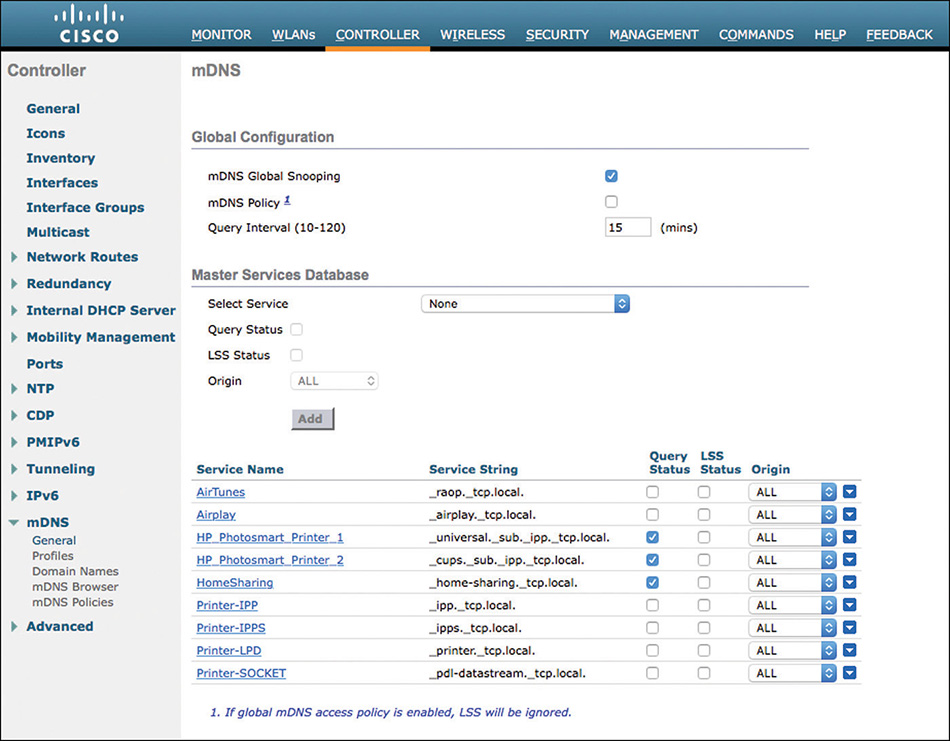
After mDNS gateway is enabled, the WLC will check the availability of supported services in each subnet, at intervals configured in the Query Interval field (CLI config mdns query interval). Default values are acceptable in the exam and in the real world, because they match the iOS and macOS timer behaviors. It may happen that Apple would change the default timers and that new values would be recommended, but such a change is unlikely to happen without the AireOS default timers being adjusted accordingly.
You also need to select which services you want to be supported (and relayed) by this WLC. A default list exists at the bottom of the page. You can delete services, or add services with Select Service (Select Service and click add; CLI config mdns service). You can also check or uncheck Query status (when adding a service, in the Master Services Database section, or after the service is added, in the list of services at the bottom of the page) if you do not want the WLC to send availability queries for specific services.
There may be WLANs where you do not want mDNS, which is a form of multicast, to be forwarded. For this reason, you also need to activate mDNS selectively on the WLANs where mDNS matters. You can activate mDNS forwarding from the WLAN Advanced tab by checking the mDNS Snooping option (CLI config wlan mdns enable).
Note
The WLC advertises the services from the wired devices (such as Apple TVs) learned over VLANs, when
mDNS snooping is enabled in the WLAN Advanced options.
An mDNS profile is enabled either at interface group (if available), interface, or in the WLAN (see below).
You do not need to enable Multicast or IGMP snooping to activate support for mDNS. mDNS is treated as a special service outside the Multicast configuration scope, even if mDNS uses multicast.
These commands configure the mDNS gateway function on the AireOS WLC. On switches, you can also enable the same type of gateway functions for wired mDNS devices that are not in the same VLAN. This type of configuration is independent from your AireOS WLC configuration, but they nicely complement each other to allow for an end-to-end mDNS support strategy. You can find more information in the IOS Service Discovery Gateway (SDG) configuration document: https://www.cisco.com/c/en/us/td/docs/ios-xml/ios/ipaddr_dns/configuration/15-sy/dns-15-sy-book/Service-Discovery-Gateway.html.
mDNS Profiles
The general configuration just described means that all services will be potentially advertised to all interfaces or WLANs. In many cases, you will want to restrict the list of services supported on some interfaces (for example, to avoid those TV services from being advertised in a classroom WLAN). To create such a shorter list of services, you create a profile. After creating a profile, you map the profile to an interface group, an interface, or a WLAN. Clients receive service advertisements only for the services associated with the profile.
Profiles are created from Controller > mDNS > Profiles. You cannot delete the default profile, but you can create a new one. Edit the new profile and add services to that profile (CLI config mdns profile).
After the profile is created, you can map it to an interface group (from Controller > Interface Groups > Edit group > pick a profile name for the mDNS Profile drop-down list; CLI config interface group mdns-profile), an interface (from Controller > Interfaces > Edit interface > pick a profile name for the mDNS Profile drop-down list; CLI config interface mdns-profile), or a WLAN (from WLANs > Edit WLAN > Advanced > pick a profile name for the mDNS Profile drop-down list; CLI config wlan mdns profile).
You may end up with a WLAN with a profile and an interface or interface group with a different profile. What happens to a client in that WLAN where traffic is sent to that interface? The highest priority is given to the profiles associated with interface groups, followed by the interface profiles, and then the WLAN profiles. Each client is mapped to a profile based on the order of priority. So in this case, the client will receive the profile associated with the interface.
mDNS AP
At this point, your WLC learns services from wireless devices and from wired devices; however, mDNS is not routable. Therefore, your WLC will learn only about wired services that are in the same subnet as your WLC’s interfaces; that is, VLANs that are “visible” to the WLC (and likely close to your WLC, as the trend is to limit the scope of VLANs to a single or limited set of switches). Your WLC will not learn about wired services on switches to which your APs connect, if they are in different subnets/VLANs (and different switches) that are not Layer 2 visible to the WLC. To enable the AP to encapsulate into CAPWAP and send to the WLC the services it detects on its switch, enable mDNS AP.
Note
The AP will detect only wired services in its VLAN. If you want the AP to detect services in more than one VLAN, set the AP port to trunk, with the AP intended VLAN as the native VLAN.
The AP can snoop up to 10 VLANs, so you may have to limit the number of VLANs on the AP trunk (with the switchport trunk allowed vlan interface command), and those VLANs should also be configured at the mDNS AP feature level, because the WLC has to understand the VLAN tags forwarded by the AP along with the service information.
To enable mDNS AP, navigate to the target AP (in Wireless) Advanced tab and check mDNS Snooping. After mDNS snooping is enabled, you can also configure the list of VLANs to snoop (CLI config mdns ap enable/disable <APName/all> vlan <vlan-id>).
mDNS Filtering Options: Priority MAC, Origin, and LSS
At this point, your WLC may start to be overloaded with service announcements from wireless and wired locations. There are a few ways to limit the amount of traffic. The first mechanism is to ensure that the most important services are always on top (always present in the list of services, even if the list exceeds the max number of entries on your WLC platform). This feature is called Priority MAC. From the Controller > mDNS General page, select a service at the bottom of the page or add a service. In the Service Detail page, at the bottom, you can associate the priority MAC to that service, as shown in Figure 7-44.
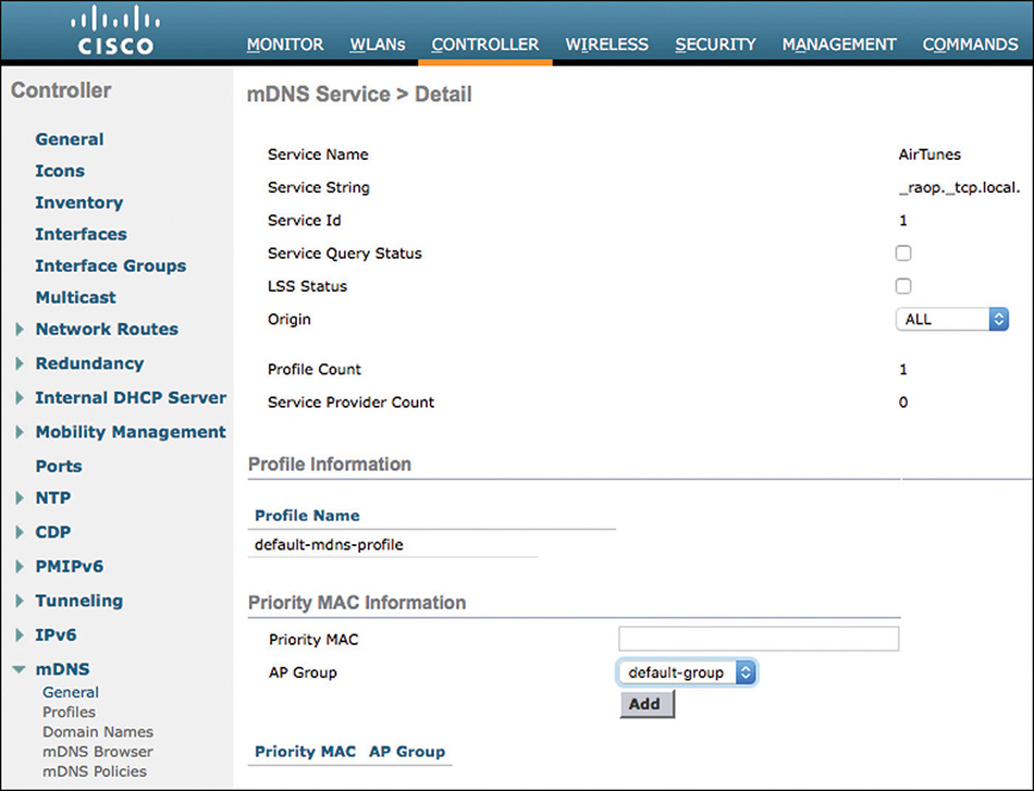
This will ensure that the device (whose MAC address you entered) advertising this service will always be on top of the list (CLI config mdns service priority-mac). Notice that you can limit this priority to a specific AP group. This may be useful, for example, if you want the local printer to be always the one advertised in a given building or floor to which an AP group is associated, but another printer would be prioritized for another floor and another AP group.
Origin-Based Service Discovery
After a service is configured, it will be learned from wired/wireless. However, you can decide whether a given service should be learned only from Wired or Wireless (or both). This is done simply from the Controller > mDNS > General page. For each service listed, you can set the Origin to All, Wired, or Wireless.
Note
Keep in mind that Origin works inbound. You filter if the service should be discovered from wired sources, wireless sources, or both. Origin does not say that a service should not be advertised to wireless, for example. To configure outbound policies, use Profiles (or policies) and associate them to a WLAN or an interface.
If you configure a service for LSS, you apply a restriction that is wireless only (LSS does not work for wired services). Therefore, if a service is set for LSS, you cannot configure it to be “wired only.”
LSS
In some cases, you may want to limit mDNS exchanges to devices on a given AP (regardless of the SSID) or a set of neighboring APs. A typical example is a large (or densely populated) classroom with two or three APs, where iPads communicate with the local wireless Apple TV, and the like, but should not communicate with an Apple TV on the other side of the school (typically because there would be potentially tens of Apple TVs to choose from every time, and this would not be practical). This type of filtering is called Location Specific Services (LSS).
LSS is also simply configured on a per service level, in Controller > mDNS > General. You can check LSS for any service already present or that you add. When you click Apply, each service for which LSS is enabled will add the MAC addresses of the APs from which it is learned. Wireless clients requesting that service will receive responses only for the services that have the same AP MAC address mapping as the requesting client, or whose AP MAC address tag is one AP in the local AP list of RF neighbors. This way, your clients will see local services and services available through neighboring APs, but not beyond. This helps reduce the scope of visible services. With this feature, you see only services around you (for example, a printer), instead of seeing all the services in the building. (If you want a printer near you, you do not want to have to browse through all printers in all buildings and all floors of your campus every time.)
Note
Keep in mind that the LSS filter works only for wireless clients and wireless services, not for wired services. The client requesting a service will also receive responses from the snooped services that the WLC knows about, regardless of their location, unless you configure further filters (policies follow).
mDNS Policies
Filtering per location or origin is efficient in smaller networks. In larger networks, stricter policies are required. Bonjour policies allow per service instance (MAC address) configuration that mandates how the service instance is shared:
Service instance is shared with whom (user-id)?
Service instance is shared with which role(s) (client-role)?
What is the location allowed to access the service instance (client location)?
This configuration can be applied to wired and wireless service instances, and the response to any query will solely be based on the policy configured for each service instance. This allows selective sharing of service instances based on the location, user-id, or role. Because most service publishing devices are wired, this allows filtering of wired services at par with wireless service instances. While an mDNS profile associated with the client checks for service type being queried before responding to the query, the access policy further allows filtering of specific service instances based on querying client location, role, or user-id.
To configure this type of filtering, you start by creating service groups. A service group is a name associated with a set of MAC addresses. Each MAC address is configured with a unique name, which can be the service instance name, and the location of the MAC address for both wired and or wireless. The location can be an AP, an AP group, or an AP location. An AP location is particularly useful if you expect users to roam (and if no AP group matches the roaming domain). You can use the location name (setting the same location name on multiple APs) to determine the set of APs among which the service instance can be supported. This configuration implies that only clients from the same location as that of the device publishing the service can access the service.
Navigate to Controller > mDNS > mDNS Policies. Edit an existing mDNS Service group or create a new one. In the group configuration page shown in Figure 7-45, you can add instances and associate a name and a location (CLI config mdns policy service-group).
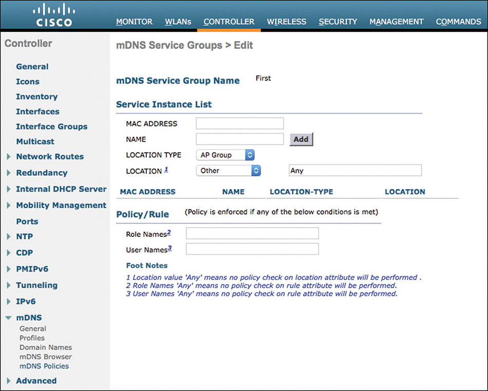
The service group also determines which users or groups should be allowed to access the instance in the group. This determination is based on a set of conditions. At the bottom of the service group page, you can configure Role Names and/or User Names. When a wireless client tries to access an mDNS service and global mDNS policy is enabled, the WLC will compare the client set of attributes to the attributes defined in each mDNS service group. If it matches the attributes defined in a service group, the client will be allowed to access only the instances that have been configured in that service group.
Your service group already has instances that match a location type and name. If these are the only attributes that you need, you can set the role and user names to Any, or leave the fields empty.
Alternatively, you can set a role name (for example, students), and even a username if you want to restrict the service to a single user (CLI config mdns policy service-group user-role | user-name).
If you configure a role or a username, the authenticating user will need to receive such an attribute. This is done with AAA override enabled in the WLAN and an authorization profile in ISE that will associate the user with the role name. Your ISE authorization profile can also point directly to an mDNS profile name.
Note
For a sample configuration, see https://www.cisco.com/c/en/us/td/docs/wireless/controller/technotes/8-0/WLAN-Bonjour-DG.html.
If you do not use AAA override, you can also use local policies (in Security > Local Policies) to identify a device type and associate an mDNS profile to that local policy. The local policy can also target a role string obtained via AAA override.
AireOS Configuration Summary
Most of the best practice configurations are enabled by applying the Fastlane macro on an SSID. Study what this macro configures and you will know most of the best practices for AireOS QoS. The only exception is ACM, which should be enabled only on a case-by-case basis. In 8.3, Fastlane enables CAC automatically (later codes do not), but you can disable ACM if needed (or asked). Keep CAC if most of your clients are Apple and/or hard phones. Disable CAC if most of your clients are of different categories (Windows, Android).
There is no best practice configuration for AVC or for Bonjour/mDNS. The lab questions will dictate what should be configured and how. In the real world, AVC may have some impact on your WLC CPU (or not!), so you should test your AVC configuration before deploying it widely.
Autonomous APs
AireOS configuration for application services support is extensive, and that’s because AireOS needs to support large and small networks in any vertical. By contrast, autonomous APs have a much smaller configuration span for QoS and real-time applications. There are two main reasons for this smaller feature scope:
Autonomous APs are primarily intended for locations with a small number of APs. In such locations, you expect a simpler client structure and less roaming concerns. In other words, you do not expect a heavy traffic competition with high user density and intense roaming.
Autonomous APs are primarily Layer 2 bridges. Their main purpose is to translate between two Layer 2 mediums (802.11 and 802.1). The management of application priority is expected to be done upstream (Layer 3 devices or applications).
This does not mean that there is no awareness of Layer 3 QoS (DSCP) in autonomous APs. It means that autonomous APs do not perform DPI. Autonomous APs simply look at frames and packet headers and apply translation rules between mediums based on the header values. This translation results in the following domains:
DSCP to UP: Decide which wired QoS value (802.1p, or DSCP) should translate into which 802.11 User Priority.
Retry options: Customize the rates and retries allowed for each UP.
EDCA Parameters: Customize each UP parameter (AIFSN, TXOP, CW).
“Advanced features”: Apply customization parameters designed for autonomous APs and voice traffic optimization.
DSCP to UP Mapping
The autonomous AP GUI includes a Services > QoS page, shown in Figure 7-46. You should know its content well.
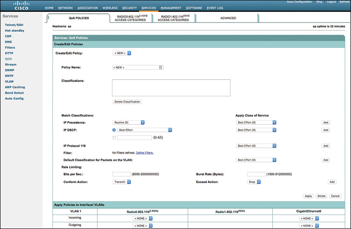
On the QoS policies tab, you can create a customized mapping between wired QoS and 802.11 QoS values. You can also associate this mapping to a rate limiting configuration.
In the GUI, create a new policy name. In the match classification area, select which DSCP value should translate to which UP.
Notice that the UPs are named after the original 802.1p-1998 table examined at the beginning of this chapter. To help the Wi-Fi administrator unfamiliar with the 1998 802.1p nomenclature, the intent of voice (<10 ms latency [6]) and video (<100 ms latency [5]) are expressed. In a typical setup, you would at least create a policy for voice. Creating a policy that includes both voice and video traffic mapping is acceptable, too, but the video part is often left aside (because the primary concern is the audio experience). In any case, make sure to respect the recommended mapping:
Expedited Forwarding (EF) -> UP 6
Assured Forwarding Class 4 Low (AF41) -> UP 5
From the GUI, create your policy, add a voice mapping rule, then click Apply, as shown in Figure 7-47. You can also add a video rule if needed.
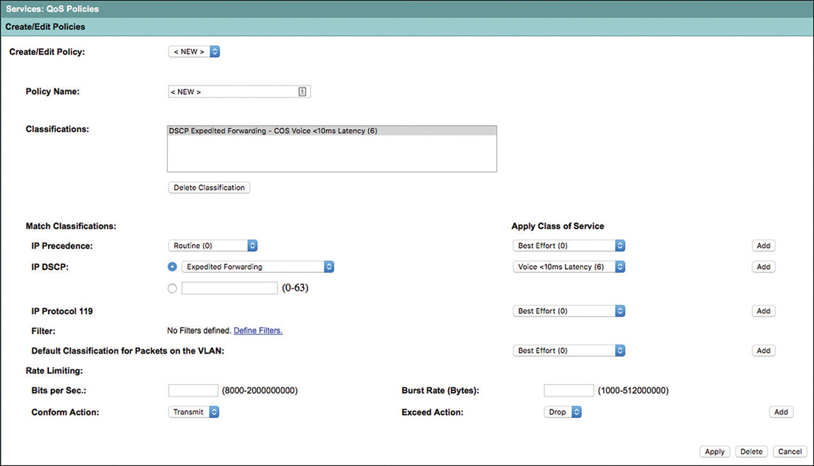
From the CLI, you will use the class-map command. The GUI forces the class-map creation to the “match-all” argument. This forces you to create one class map per traffic marking type (your incoming packet cannot have AF41 AND EF marking at the same time, on the same packet). This is acceptable and common. However, the CLI allows you to mimic the GUI (match-all) or to use match-any, which allows you to target voice or video marking in a single class map. This last option is not the most elegant, but is also acceptable on an AP where the QoS rule set is very simple and static:
class-map match-all _class_RealTime1
 match ip dscp ef
class-map match-all _class_RealTime0
 match ip dscp af41
!
policy-map RealTime
 class _class_RealTime0
  set cos 5
 class _class_RealTime1
  set cos 6
Each class map targeting specific traffic (identified by its DSCP value) is created first. Then a policy map is created. Inside this policy map, you call each class, one at a time, and determine what marking this class should receive. The link between the class map DSCP and the marking policy for that class in the policy map creates the marking mapping.
Notice that the QoS mapping set is CoS, not UP. This is consistent with the GUI, and with the logic where the UP maps to 802.1p-1998. One advantage of this simplified map is that it can be applied in any direction, on any interface.
In most autonomous networks, it would still be common to create a voice SSID and a data SSID on the same radios (or voice in 5 GHz and data in 2.4 GHz), but sent to different VLANs.
You would therefore create a second policy mapping Best Effort to Best Effort 0.
You then need to apply the policies to interfaces. They can be physical interfaces (2.4 GHz, 5 GHz radios or Ethernet interface) or subinterfaces (VLAN values on physical interfaces). In most cases, applying the policy everywhere is the simplest course of action. In Figure 7-48, VLAN 1 exists on the 2.4 GHz radio and VLAN 12 on the 5 GHz radio. Data traffic is sent to the SSID on the 2.4 GHz radio and VLAN 1, and voice traffic is sent to the 5 GHz radio SSID and VLAN 12.
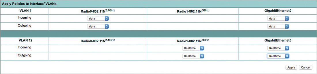
Applying the Data policy to everything VLAN 1 and the Voice policy to everything VLAN 12 is simple and efficient.
In the context of the CCIE Wireless exam, you also need to carefully examine what you are attempting to achieve (and what the question states). If your policy only does remarking, an Ethernet incoming policy will ensure the correct mapping as the wired packet transits through the AP toward any radio interface. Therefore, there is no reason to apply the policy both on the incoming direction of the Ethernet interface and on the outgoing direction of a VLAN or radio (you make the AP do the work twice).
The preceding holds true if your expected traffic flows with a simple structure (from wired to wireless). However, if you expect traffic to flow from one radio to the other, then positioning the policy at the radio outgoing direction makes more sense.
The same logic applies for the reverse direction.
In summary:
Apply the policy to both wired and wireless incoming direction if the traffic is expected to flow between a given SSID and the wired network. Do not apply the policy to the outbound direction on any interface.
Apply the policy to both wired and wireless outgoing directions if the traffic is expected to flow between a given SSID and another SSID, as well as between a given SSID and the wired network. Also, applying the policy to the incoming direction is then optional (but acceptable).
The CLI command to apply the policy follows a particular logic.
The policy is applied to either the interface level or the subinterface level (if VLANs were created). The following example shows subinterfaces for VLAN 1 and VLAN 12 (following the GUI example structure).
The policy is called at the subinterface level with the command service-policy and the direction:
interface Dot11Radio0.1
 service-policy input Data
 service-policy output Data
 interface Dot11Radio1.12
 service-policy input RealT
 service-policy output RealT
interface GigabitEthernet0.1
 service-policy input Data
 service-policy output Data
interface GigabitEthernet0.12
 service-policy input RealT
 service-policy output RealT
You can add bandwidth control along with the remarking policy. The GUI does not let you create both (bandwidth options with class of service mapping), but you can create a new policy that provides bandwidth selection. You then have the option to define a rate limit value and a burst rate.
Be careful, the rate limit is in bits (binary 0 or 1) per second, burst is in bytes (octets).
In the CLI, the rate limit can be added to a marking policy or be an independent policy. Inside the policy map, you still call the class, and then decide the rate limit with the policy command. For example:
Class Map match-all _class_BW0
Match any
Policy-map ratelimit
Class _class_BW0
police 30000 50000 conform-action transmit exceed-action drop
The CLI offers more options (bandwidth, and so on). However, configuring such bandwidth control on a Layer 2 bridge is uncommon.
In a standard QoS logic, such policy is applied to the outgoing direction of an interface. (In the incoming direction, the packet is already there. You do not need to control what comes, you just need to receive it.)
Such bandwidth limitation is possible on the GUI. You would apply it in the outgoing direction of a subinterface (with the standard service=policy command). You can also apply it to a WLAN, as shown in Figure 7-49. In that case, the rate limit is configured in the GUI from the SSID itself (Security > SSID Manager > Edit SSID > Rate Limit Parameters).
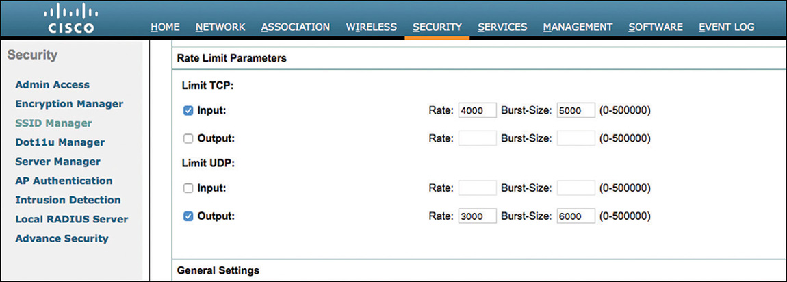
The CLI equivalent is done under the SSID configuration in global mode, for example:
dot11 ssid Test1
   vlan 12
   rate-limit tcp input data-rate 4000 burst-size 5000
   rate-limit udp output data-rate 3000 burst-size 6000
In real life, you are more likely to need a WLAN-specific rate limit than an interface policing. In both cases, you would prefer working with marking than creating bandwidth limits, as explained at the beginning of this chapter. In the exam, read carefully to verify where the bandwidth is expected to be controlled.
Retry Options
Having different types of traffic mapped to different UPs is critical. However, you also know that voice traffic is time sensitive. Getting statistical advantage in the medium access with UP 6 is great, but IOS also allows you to configure two more options (that are not present in AireOS): the retry count for each UP and the rate shifting options for these UPs. AireOS uses an internal timer logic for voice that can be configured in the EDCA parameter page (Low Latency MAC—this feature enables a 30 ms timer that drops voice frames that stay in the AP buffer for more than that duration).
This option was not covered in the AireOS section because it is not best practice. (Do not use it unless you are in a lab and someone asks you to turn it on.) In most cases, it is better to let the end device manage its buffer than to decide at the AP level whether the device buffer is about to get empty.
In the IOS world, an equivalent parameter exists and is called Low Latency Queue (LLQ). This is not something you would activate in the real world unless you are addressing a very specific use case. The lab is of course a different environment in that it always asks you to solve a very specific use case.
LLQ means that whenever a packet gets in the AP buffer, it will always be sent first (before packets in other queues are dequeued), giving delay-sensitive data preferential treatment over other traffic.
This means that you can prioritize traffic on an IOS AP with three methods:
With the policy map method, you may just tag, which says “this packet is urgent” but does not apply any priority per se.
There is a QoS Elements for Wireless phones option (discussed next) that prioritizes any voice packet regardless of any other consideration. This is an LLQ “by nature,” without any upper limit.
With the LLQ option queue configured here, you define how many times the AP should try to send each voice packet, and at what speed, before giving up and trying the next packet.
LLQ is configured in Services > Stream > Radio0 or Radio1.
Set Cos 6 (Voice) to Low Latency Queue, as shown in Figure 7-50.
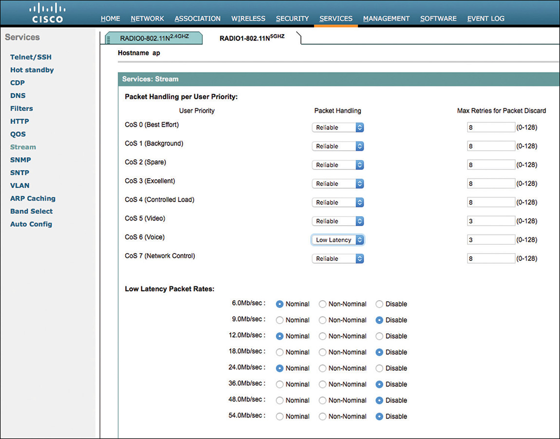
This configuration enables you to configure how many times the AP radio should attempt to send a voice packet before dropping that unsuccessful packet and sending the next one. This is the Max retries for Packet Discard value. The default value is 3. Keep in mind that this means that after three attempts, the AP will drop an unsuccessful voice packet. By contrast, all other queues seem to retry “forever” (as the configuration is “reliable,” which seems to mean “retry until ACK is received”). In reality, the AP max retry can also be configured from its default maximum (see the “Autonomous APs” section of this chapter).
Notice that the low latency does not create any prioritization per se. It simply says “As this queue is otherwise configured as a priority queue, allow me to configure how many times the AP should try to send each packet of that type before dropping it if the packet cannot be sent successfully.” You can set several user priorities to low latency, and set the max retries for each of them.
After you have defined the retry level, you can also configure at which speed those frames should be sent. This is done at the bottom of the page, in the Low Latency Packet Rates section. You can set each rate to the following:
Nominal: The AP will try to use this rate to send the low latency packets (using the faster rate first, and of course depending on the client signal level).
Non-nominal: The AP will try not to use that rate but will revert to it if no nominal rate is possible.
Disabled: The AP will not try to use that rate.
For example, in Figure 7-50, if your AP to client RSSI level is good enough to try 36 Mbps, the AP will try 24 Mbps (first nominal rate at or below the client possible rate), then revert to 12 Mbps if 24 Mbps fails.
Suppose that 24 Mbps and 6 Mbps are set to Nominal, and 12 Mbps is set to Non-nominal (other rates are disabled). The AP would try 24 Mbps first, then 6 Mbps, then 12 Mbps if none of the nominal rate attempts were successful.
So good practices are to set the rates you want to use as Nominal, then set one low rate as Non-nominal, so that the AP has a plan B in case all possible nominal rates fail. Disable all other slow rates.
In the CLI, these elements are configured at radio level. For example:
Int do 1
traffic-stream priority 6 sta-rates nom-6.0 nom-12.0 nom-24.0
 packet max-retries 3 0 fail-threshold 100 500 priority 6 drop-packet
 packet speed  6.0 12.0 24.0 priority 6
The CLI version is obviously more complex. The traffic-stream command determines the nominal and non-nominal rates for each configured UP set to LLQ.
The packet speed command seems to repeat the traffic-stream command. In fact, the traffic-stream command defines the nominal and non-nominal rates, whereas the packet speed command lists all the allowed rates for that same UP. The rates not listed in packet speed are disabled rates (while traffic-stream does not define disabled rates). In a properly configured AP, the rates listed on both lines should be the same, packet speed defining the allowed rates and traffic-stream defining which of these rates are nominal and which are non-nominal.
The packet max-retries command sets the LLQ, stating that the AP will try three times. This command structure is complex because it uses four numbers (3, 0, 100, and 500). Its logic is as follows (starting from the first packet the AP sends to a given client): The AP will try each UP 6 packet to a given client three times. If the packet fails three times, the AP drops that packet and attempts to send the next one.
How many failed consecutive packets would the AP try this way? In this configuration, 100. If 100 consecutive packets fail (try three times, drop and try next), then the command considers that a threshold is reached and allows for a different logic to be tried (for example, try eight times instead of three).
In the default version of this command the new logic is to stop trying three times (the reasoning is that this client is obviously unreachable, if the AP failed 100 consecutive packets, each with three attempts). The AP sends each packet only once (retry is 0) and attempts 500 more packets.
If these 500 more packets failed (no ACK), the AP drops the packets for that client (this is the drop packet option at the end; without that option, the AP disconnects the client). With drop packet, the AP kindly restarts its counters without disconnecting the client.
EDCA Parameters
Configuring bandwidth control is uncommon because the queuing mechanisms on the radio interface use 802.11e parallel queuing with CW and other 802.11-specific parameters. Attempting to use wired-type bandwidth control with policing or shaping is often seen as an attempt to square circles, using tools that are not adapted to the constraints of 802.11 transmission mechanisms.
It is, however, more common to tune the 802.11 parameters for transmission control for each QoS category, with CW, slot time (that is, AIFSN), and TXOP durations.
These parameters are configured in the Radio [2.4 | 5] GHz Access categories page as shown in Figure 7-51. In most cases, you want to check the Optimized Voice or the WFA Default check box and apply. You could be asked to customize the values, which implies the skill to copy numbers into fields.
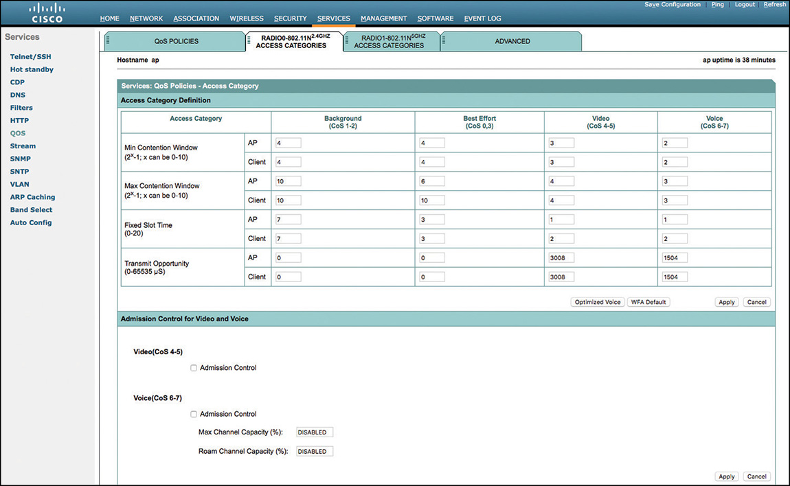
If you prefer to use the CLI, you would go to the target radio interface and configure the values for each class where you want special treatment. You would then apply these values both for the WLANs (“cell”) and the radio (“local”). For example:
Interface do 1
dot11 qos class video both
    cw-min 5
    cw-max 6
    fixed-slot 8
    transmit-op 2
Note
Please do not take these semi-random numbers as best practices. The correct numbers are the ones defined for Fastlane EDCA values as explained at the beginning of this chapter, or the values expressed in the Optimized Voice and WFA Default options.
The preceding is simple because you create the rules once and apply them for both cell and local. However, there may be cases where you need to create both the local and the cell rules. You may want to get into the habit of creating two identical sets of rules, one for cell and one for local:
Interface do 1
dot11 qos class video cell
    cw-min 5
    cw-max 6
    fixed-slot 8
    transmit-op 2
dot11 qos class video local
    cw-min 5
    cw-max 6
    fixed-slot 8
    transmit-op 2
As you control the transmission counting mechanism, you may also be asked to control access to the UP 6 queue. This is the same CAC as on the AireOS controller. In the GUI, CAC is configured in the Same Access Category page. The recommended values are the same as in AireOS:
Voice CAC: Max Channel capacity: 50%, roam channel capacity: 6%
Video CAC: Unconfigured
In the CLI, CAC is also applied at the radio interface for local and cell usage. For example:
Interface do 1
dot11 qos class voice local
    admission-control
    admit-traffic narrowband max-channel 50 roam-channel 6
dot11 qos class voice cell
    admission-control
Notice that the values are set in the local rule, not the cell rule; however, the cell rule activates admission control, picking the CAC rule values from the local section.
In old IOS, you will also see an option to call CAC from the SSID (in the general Settings area of the WLAN). This option is not needed in recent IOS (and the one in the exam).
Advanced Features
IOS also includes customizations intended to improve the performance of voice traffic. Most of them are located in the Services > QoS > Advanced tab.
Prioritizing voice traffic over a wireless link on autonomous APs can be done in three ways. The first one is to create a class map, a policy map, and a service policy, then set a higher bandwidth or priority level to voice traffic. This is what the previous Policy section was about. But in an autonomous AP (remember, a Layer 2 bridge), applying a QoS tag (DSCP, CoS, or 802.11e) only partially solves the problem. The DSCP or CoS tag will simply label the frame as urgent or not. Putting the frame in an 802.11e category based on its tag (EF in CoS 6, for example) helps, because each queue is treated differently in the AP buffer, and the voice queue is statically prioritized over the other queues. If there are too many voice packets, using CAC can also prevent having voice packets starve the other queues.
But if there are many “other types” of packets, and few voice packets in between, putting the voice frame in UP6 may not be enough. Your voice packets may be delayed because other larger packets are filling up the AP queues. To enhance the prioritization, you may need to add another feature that would always prioritize voice packets. This feature is called QoS Element for Wireless Phones and can be found in Services > QoS > Advanced, as shown in Figure 7-52.
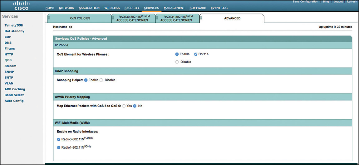
Enabling QoS Element for Wireless phones generates two behaviors:
The AP prioritizes voice packets over the wireless links, regardless of any QoS configuration.
The AP sends in its beacon an additional information element called QoS Basic Service Set Load Information Element, or QBSS Load IE. This information element mentions how many clients are associated to the SSID, and what the AP utilization percentage is. Roaming devices can use this information to decide which AP is the best candidate to join (having more space and fewer clients). This information can be sent in a Cisco-proprietary and pre-802.11e way (by just checking QoS Element for Wireless Phones), or using the IEEE 802.11e format (by also checking the Dot11e check box).
Both policy map (when bandwidth is reserved for the voice stream) and QoS Element for Wireless Phones can prioritize voice packets. It all depends on whether you want to use a policy map, for which the configuration method would be the same on most IOS devices, or use configuration commands specific to autonomous IOS APs.
Notice that if you use the Dot11e method, you need to have WMM enabled on the corresponding interface. This is configured at the bottom of the same page, and WMM is enabled on both interfaces by default.
If you disable WMM, you may still be able to use QoS Element for Wireless Phones, but the AP will not broadcast the QBSS Load Information Element using the 802.11e format; it will use the Cisco CCX format.
The QoS Element for Wireless Phones can be configured with the following command:
ap(config)# dot11 phone dot11e
Remove the dot11e if you want to use the CCX QBSS Load element instead of the 802.11e format.
Another option that is part of the good practices and located in the same page is to set the AVVID Policy mapping to Yes. In wireless, voice is CoS 6. Cisco follows the IETF recommendations on the wired side and 802.1p tag 5. Checking AVVID priority mapping allows a transparent translation from 5 to 6 and back when packets transit through the AP. In most networks, you will use DSCP, but this option ensures that 802.1p markings are correctly interpreted. This is also a global CLI command:
ap(config)# dot11 priority-map avvid
Another element of good practice when configuring a voice WLAN is ARP caching. Because you do not want your wireless phone to fail due to an ARP request delay, enable ARP caching on the AP and check the Forward ARP Request to Radio Interfaces option to make sure that the AP knows all MAC addresses of all IP clients. In the GUI, this option is configured in Services > ARP Caching, as shown in Figure 7-53.
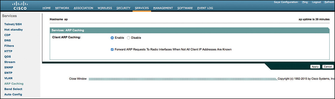
In the CLI, this is also a global command:
Ap(config)# dot11 arp-cache optional
The optional keyword is the forwarding to radio interface optional part.
Autonomous Application Service Configuration Summary
IOS AP configuration for supporting application services sometimes looks like a disconnected collection of items, without clear flow. The reason may be that autonomous APs are Layer 2 bridges. They are not intended to collect, store, examine traffic, and then decide the best fate and path based on the traffic type. They are intended to convert 802.11 headers into 802.1 headers and back. Anything above is optional. In a lab, the “above” will match the question you are asked. In the real world, there are a few items that are considered as best practices:
Keep WWM to enabled (in Services > QoS > Advanced).
Set the AVVID mapping policy (same location).
Enable ARP caching (in Services > ARP Caching).
If you use voice, set the Access Categories for the matching radio to voice optimized of Fastlane values (in Services > QoS > radio > Access Categories).
Use marking map policies to ensure that DSCPs mark to the right CoS and UPs. Rate limiting is not preferred (use marking and the natural prioritization of marking instead, as explained in the first part of this chapter).
CAC is optional (turn it on if most of your clients are TSPEC enabled). Notice that IOS has no trust-exceptions for Apple iOS or Mac OS clients. With CAC enabled, these clients won’t access the UP 6 queue (because they do not support TSPEC).
LLQ configuration is uncommon and optional (let the clients manage their buffer; don’t think that the AP can know whether a packet is “late”).
Wired Configuration
The CCIE Wireless exam tests your knowledge of Wi-Fi. However, it would be an illusion to think that the network you care about (and therefore your skills) stop at the AP or WLC level. Clearly, there would be, in any network, a large number of other specialists to take over where you left off and configure routing, wired QoS, Unified Communications, deep Security, and so on. However, you should not think that there is no reason for you to know anything about these fields. In fact, you should aspire to be independent, face any network on your own, and survive any configuration request, even if the request has an impact on the wired infrastructure and no campus LAN Switching specialist is there to help you.
In the application services field, this autonomy implies being able to configure basic QoS on a switch. Such an ability covers two fields:
The ability to use DSCP or 802.1p when making a switching decision
The ability to create marking and queueing policies on a switch
Trusting DSCP or CoS
Most switches receive traffic on access ports and trunk ports. On access ports, QoS is expressed only in the Layer 3 DSCP field. Trunk ports can receive traffic that includes an 802.1Q header, which includes an 802.1D/802.1p Layer 2 QoS value. You can configure the switch to use the Layer 3 DSCP value or the Layer 2 CoS value, to decide the fate of the incoming packet. The best practice, in the context of wireless, is to use DSCP, because it expresses the end-to-end intent of the packet (refer to the first part of this chapter). Although a switch is a Layer 2 device, most switches can work with Layer 3 and recognize DSCP. The value you use (DSCP or CoS) is set by the trust value:
SwitchA(config-if)# interface f0/2
SwitchA(config-if)# mls qos trust dscp
Notice that in IOS XE switches, DSCP is trusted by default. Some other, older switch platforms (for example, 3750s) require you to use the mls qos global command to activate QoS (and therefore the trust mechanism). You are unlikely to face such an older switch in the exam. In real life, on an older switch, you are expected to enter mls qos before any trust command.
Trusting DSCP means that the switch will look at the DSCP field of the incoming traffic on the configured port to decide the packet remarking. The outbound buffers will still be built using Layer 2 queues. The trust function is to decide the field that will be used to direct the incoming packet to the right queue.
Note
This Layer 2–based outgoing queuing logic is the reason why some “experts” will tell you that switches can only work with Layer 2 QoS. This is a basic misunderstanding of the problem that trust is solving. Its purpose is not to work on the outgoing queuing but to decide which field should be used on the incoming packet to decide the outbound, Layer 2–based queue. Using DSCP for that purpose is best.
Your port may be a trunk (in which case both DSCP and CoS will be available) or an access port (in which case no CoS is available, and trust DSCP is the only option). In that case, the port may connect a phone behind which a laptop connects. This port will then have both a data and a voice VLAN configured per the following example structure:
SwitchC(config)# interface g0/21
SwitchC(config-if)# power inline auto
SwitchC(config-if)# cdp enable
SwitchC(config-if)# switchport mode access
SwitchC(config-if)# switchport access vlan 10
SwitchC(config-if)# switchport voice vlan 20
SwitchC(config-if)# trust device cisco-phone
SwitchC(config-if)# trust cos
Two key elements are to be examined from this configuration. You set a data VLAN and a voice VLAN. CDP will be used to recognize a Cisco phone, and QoS marking from this phone will be trusted. Cisco phones are an exception to the DSCP rule because they mark only CoS.
The mls qos trust command has different options depending on the platform. Using the “?” after the trust keyword, you will recognize which option states that you would trust the marking coming from a Cisco phone.
On all ports connecting an AP (in local mode or FlexConnect mode) or a WLC, you will trust DSCP (trust dscp is the default and only option on most IOS-XE switches):
SwitchC(config)# interface g0/21
SwitchC(config-if)# description  *** to WLC ***
SwitchC(config-if)# switchport mode trunk
SwitchC(config-if)# mls qos trust dscp

SwitchC(config)# interface g0/21
SwitchC(config-if)# description  *** to local mode AP ***
SwitchC(config-if)# switchport mode access
SwitchC(config-if)# mls qos trust dscp

SwitchC(config)# interface g0/21
SwitchC(config-if)# description  *** to FlexConnect AP ***
SwitchC(config-if)# switchport mode trunk
SwitchC(config-if)# mls qos trust dscp
Your WLC typically connects to a trunk, and its management interface should be tagged (that is, not “0,” or untagged, as you configure the interface in the WLC initial setup) for security purposes. In older codes, you used to trust CoS. In 8.x codes, you trust DSCP, as explained at the beginning of this chapter.
The local mode AP case is obvious because it is on an access port. (There is no CoS, only DSCP.)
The FlexConnect AP has its management IP address (the address used to communicate with the WLC) on the native VLAN (which has no 802.1Q field). Therefore, you must trust DSCP in order to catch management tagging (CAPWAP control for example, tagged as CS6). If you were to trust CoS, the management traffic (on the native VLAN, without 802.1Q field) would appear as “untagged” and would be treated as best effort, even if its DSCP marking is CS6.
QoS Policies
Making sure that you trust DSCP is the first QoS task on your switches. The other task is setting rules and policies, just like you did on the autonomous AP.
The logic is similar to that of the autonomous AP CLI. You create class maps that target specific traffic (based in existing marking or source/destination pairs, for example), the policy maps that decide what should happen to the targeted traffic. You then apply these policies to interfaces.
Class Maps
Class maps can target a wide range of ways of recognizing traffic type. You do not need to know all possible ways, but the most common are as follows.
Start by creating an access list for voice traffic. Voice uses UDP ports between 16384 and 32767.
sw(config)# access-list 101 permit udp any any range 16384 32767
Next, create a class map matching this access list:
sw(config)# class-map voice_ports
sw(config-cmap)# match access-group 101
Repeat the same operation for signaling or other traffic that you can recognize based on their port:
sw(config)# access-list 102 permit tcp any any eq 2000
sw(config)# access-list 102 permit udp any any eq 1720
sw(config)# class-map signaling_ports
sw(config-cmap)# match access-group 102
sw(config-cmap)# exit
Creating class maps by recognizing traffic targeted with an access list is very common, and you should be familiar with this technique. You can also target a specific DSCP or CoS value (just like in the autonomous section):
sw(config)# class-map Voice
sw(config-cmap)# match dscp ef
sw(config-cmap)# exit
Policy Maps
After you have class maps, you can create policy maps that call each class map in turn and decide the QoS marking for traffic in that class. For example:
sw(config)# policy-map VOIP3
sw(config-pmap)# class voice_ports
sw(config-pmap-c)# set dscp ef
sw(config-pmap-c)# exit
sw(config-pmap)# class signaling_ports
sw(config-pmap-c)# set dscp CS3
sw(config-pmap)# exit
sw(config-cmap)# exit
Service Policy
After the various policy maps are created, you apply them to the interfaces of your choice. For example:
sw(config)# interface g1/0/1
sw(config-if)# service-policy output VOIP3
Notice that the span of possibilities will depend on your switch platform. In general, you can create remarking policies inbound or outbound, although it makes more sense to remark traffic as you receive it (inbound), instead of keeping the wrong marking as the traffic traverses your switch, and only caring about making the marking right when traffic leaves your switch. This is a general recommendation, but the CLI will allow you to remark wherever you want (on most platforms).
You can also set bandwidth limitations with police, bandwidth, shaping, and many other commands. The details of which option is best, based on the intent of your configuration, is more in the realm of QoS and voice specialist than in that of a wireless expert. However, you should keep in mind that bandwidth control usually makes sense only outbound. When traffic reaches your switch you want to receive it and mark it properly, but it is too late to decide how much of that traffic you should accept (you are on the passive, receiving side of the link). It is only when you send traffic outbound that you should decide how much should be sent, and this is where bandwidth limiting configurations make sense.
Summary
The first part of this chapter is key to understanding the multiple concepts behind application services configuration. Keep in mind that QoS can be expressed at Layer 2 or Layer 3. Layer 3 QoS, with DSCP and PHB, expresses the end-to-end QoS intent for the target traffic, whereas Layer 2 QoS expresses the local QoS intent, based on the local medium constraints and characteristics. A higher QoS label value typically reflects a higher sensitivity to delay, jitter, and losses. RFC 4594 (and a few others) define the common basis to classify various types of traffic and express their sensitivity to loss, jitter, and delay. On a WLC, traditional marking relied on Wi-Fi Layer 2 marking translated to (and from) Ethernet Layer 2 marking. However, the current recommendation is to use DSCP instead.
After you have defined your QoS marking policy, you can use several techniques to limit the effect of congestion: TXOP, CAC, Bandwidth contract, and QoS remarking.
You should take the time to master these concepts and train to configure them separately or together on your wireless infrastructure and neighboring switches by using the second part of this chapter. Make sure to configure multiple options and to understand what happens (make heavy use of show and debug commands). Also, configure a voice client, and use the various markings to experiment. For iOS clients, you can use a Mac OS device and Apple Configurator to create and deploy a profile that includes a whitelist. You should be able to see the marking appear or disappear while capturing whitelisted or nonwhitelisted traffic over the air (Wireshark or other). You can use a cloud application (for example, Spark or Facetime) for this test. If you test on Windows, you might need a voice application like Jabber.