
Chapter 8. Block Storage Technologies
This chapter covers the following topics:
![]() Disk Controllers and Disk Arrays
Disk Controllers and Disk Arrays
This chapter covers the following exam Objectives:
![]() 5.1 Describe storage provisioning concepts
5.1 Describe storage provisioning concepts
![]() 5.1.a Thick
5.1.a Thick
![]() 5.1.b Thin
5.1.b Thin
![]() 5.1.c RAID
5.1.c RAID
![]() 5.1.d Disk pools
5.1.d Disk pools
![]() 5.2 Describe the difference between all the storage access technologies
5.2 Describe the difference between all the storage access technologies
![]() 5.2.b Block technologies
5.2.b Block technologies
![]() 5.3 Describe basic SAN storage concepts
5.3 Describe basic SAN storage concepts
![]() 5.3.a Initiator, target, zoning
5.3.a Initiator, target, zoning
![]() 5.3.b VSAN
5.3.b VSAN
![]() 5.3.c LUN
5.3.c LUN
![]() 5.5 Describe the various Cisco storage network devices
5.5 Describe the various Cisco storage network devices
![]() 5.5.a Cisco MDS family
5.5.a Cisco MDS family
![]() 5.5.c UCS Invicta (Whiptail)
5.5.c UCS Invicta (Whiptail)
The capability to store data for later use is part of any computer system. However, how such systems write and read data in a storage device has been handled in many different ways since the beginning of computer science.
Obviously, cloud computing projects cannot avoid this topic. To actually provide self-catered services to end users, cloud architects must select a methodology to store application data that is both efficient and strikes a good balance between performance and cost. In some cases, data storage itself may be offered as a service, enabling consumers to use a cloud as their data repository.
Within such context, the CLDFND exam requires knowledge about the basic principles of block storage technologies, including provisioning concepts, storage devices, access methods, and Cisco storage network devices. This chapter starts with the most basic of these principles by providing a formal definition of what constitutes storage. It then examines different types of storage devices, hard disk drives (and associated technologies), main block storage access methods, storage-area networks (SANs), and common SAN topologies. Finally, the chapter correlates these technologies to the current state of cloud computing, providing a clear application of these technologies to dynamic cloud environments.
“Do I Know This Already?” Quiz
The “Do I Know This Already?” quiz allows you to assess whether you should read this entire chapter thoroughly or jump to the “Exam Preparation Tasks” section. If you are in doubt about your answers to these questions or your own assessment of your knowledge of the topics, read the entire chapter. Table 8-1 lists the major headings in this chapter and their corresponding “Do I Know This Already?” quiz questions. You can find the answers in Appendix A, “Answers to Pre-Assessments and Quizzes.”

1. Which of the following is a correct statement?
a. HDDs are considered primary storage.
b. DVD drives are considered secondary storage.
c. Tape libraries are considered tertiary storage.
d. RAM is not considered primary storage.
2. Which of the following represents data addressing in HDDs?
a. Bus/target/LUN
b. World Wide Name
c. Cylinder/head/sector
d. Domain/area/port
3. Which option describes an incorrect RAID level description?
a. RAID 0: Striping
b. RAID 1: Mirroring
c. RAID 6: Striping, double parity
d. RAID 10: Striping, multiple parity
4. Which of the following is not an array component?
a. SATA
b. Controller
c. JBOD
d. Disk enclosure
e. Access ports
5. Which of the following devices can potentially deploy volume thin provisioning? (Choose all that apply.)
a. JBOD
b. Storage array
c. Server
d. Dedicated appliance
e. HDD
6. Which of the following are block I/O access methods? (Choose all that apply.)
a. ATA
b. SCSI
c. SAN
d. NFS
e. SQL
7. Which of the following options is incorrect?
a. FC-0: Physical components
b. FC-1: Frame transmission and signaling
c. FC-3: Generic services
d. FC-4: ULP mapping
8. Which of the following is correct concerning Fibre Channel addressing?
a. WWNs are used for logical addressing.
b. FCIDs are used for physical addressing.
c. WWNs are used in Fibre Channel frames.
d. FSPF is used to exchange routes based on domain IDs.
e. FCIDs are assigned to N_Ports and F_Ports.
9. Which of the following is an accurate list of common SAN topologies?
a. Collapsed core, spine-leaf, core-aggregation-access
b. Collapsed core, spine-leaf, core-distribution-access
c. Collapsed core, core-edge, core-aggregation-access
d. Collapsed core, core-edge, edge-core-edge
e. Collapsed core, spine-leaf, edge-core-edge
10. Which of the following is not an advantage for the deployment of VSANs?
a. Interoperability
b. Multi-tenancy
c. Zoning replacement
d. Security
e. Isolation
11. Which of the following is incorrect about iSCSI?
a. Standardized in IETF RFC 3720.
b. Employs TCP connections to encapsulate SCSI traffic.
c. Employs TCP connections to encapsulate Fibre Channel frames.
d. Deployed by iSCSI initiators, iSCSI targets, and iSCSI gateways.
e. Initiators and targets are usually identified through IQN.
12. Which is the most popular block I/O access method for cloud offerings of Storage as a Service?
a. Fibre Channel
b. iSCSI
c. FCIP
d. iFCP
e. NFS
Foundation Topics
What Is Data Storage?
Applications should be able to receive data from and provide data to end users. To support this capability, data centers must dedicate resources to hold application data effectively while supporting at least two basic input and output (I/O) operations: writing and reading.
In parallel to the evolution of computing, data storage technologies were developed to achieve these objectives, using multiple approaches. Storage devices are generally separated into the following three distinct classes, depending on their speed, endurance, and proximity to a computer central processing unit (CPU):

![]() Primary storage: The volatile storage mechanisms in this class can be directly accessed by the CPU, usually have small capacity, and are relatively faster than other storage technologies. Primary storage is also known to as main memory, which was referred in Chapter 5, “Server Virtualization.”
Primary storage: The volatile storage mechanisms in this class can be directly accessed by the CPU, usually have small capacity, and are relatively faster than other storage technologies. Primary storage is also known to as main memory, which was referred in Chapter 5, “Server Virtualization.”
![]() Secondary storage: The devices in this class require I/O channels to transport their data to the computer system processor because they are not directly accessible to the CPU. Secondary storage devices deploy nonvolatile data, have more storage capacity than primary storage, provide longer access times, and are also known as auxiliary memory.
Secondary storage: The devices in this class require I/O channels to transport their data to the computer system processor because they are not directly accessible to the CPU. Secondary storage devices deploy nonvolatile data, have more storage capacity than primary storage, provide longer access times, and are also known as auxiliary memory.
![]() Tertiary storage: This class represents removable mass storage media whose data access time is much longer than secondary storage. These solutions are the most cost effective among all storage types, providing massive capacity for long-term periods.
Tertiary storage: This class represents removable mass storage media whose data access time is much longer than secondary storage. These solutions are the most cost effective among all storage types, providing massive capacity for long-term periods.
Figure 8-1 exemplifies these classes of storage technologies.

Figure 8-1 uses two parameters to characterize each technology: latency, which is the length of time it takes to retrieve saved data from a resource, and capacity, which represents the maximum amount of data a device can hold.
Random-access memory (RAM) provides a relatively low latency (from 8 to 30 nanoseconds) and, for that reason, is the most common main memory device. RAM chips are composed of multiple simple structures that contain transistors and capacitor sets that can store a single bit. When compared to other storage technologies, these devices have relatively low capacity (tens of gigabytes at the time of this writing).
Because the energy stored in the RAM capacitors leaks, the stored information must be constantly refreshed, characterizing the most common type of memory used today: dynamic RAM (DRAM). Represented in the bottom left of Figure 8-1, the DRAM chips (little black rectangle) are sustained by a physical structure that is commonly referred to as a memory module.
In the upper-right side of Figure 8-1, tertiary storage technologies are represented by a tape library. This rather complex system comprises multiple tape drives, abundant tape cartridges, barcode readers to identify these cartridges, and a robotic arm to load tapes to the drives after an I/O request is issued. Because of its myriad mechanical components, a tape library introduces a much longer latency (a few minutes) when compared to other storage technologies. Notwithstanding, a tape library provides an excellent method for long-term archiving because of its capacity, which is usually measured in exabytes (EB).
Depicted in the middle of Figure 8-1, hard disk drives (HDDs) epitomize the most commonly used secondary storage technology today, offering latency of around 10 ms and capacity of a few terabytes per unit. These devices offer a great cost-benefit ratio when compared to RAM and tape libraries, while avoiding the volatile characteristics of the former and the extreme latency of the latter.
The next section discusses hard disk drives, exploring the internal characteristics of this seasoned technology.
Hard Disk Drives
HDDs are widely popular storage devices whose functionality is based on multiple platters (disks) spinning around a common axis at a constant speed. Electromagnetic movable heads, positioned above and below each disk, read (or write) data by moving over the surface of the platter either toward its center or toward its edge, depending on where the data is stored.
In these devices, data is stored in concentric sectors, which embody the atomic data units of a disk and accommodate 512 bytes each. A track is the set of all sectors that a single actuator head can access when maintaining its position while the platters spin. With around 1024 tracks on a single disk, all parallel tracks from the disks form a cylinder. As a result, each specific sector in an HDD is referenced through a three-part address composed of cylinder/head/sector information.
Figure 8-2 illustrates how these components are arranged in a hard disk drive structure.

When a read operation requests data from a defined cylinder/head/sector position, the HDD mechanical actuator positions all the heads at the defined cylinder until the required sector is accessible to the defined head.
I/O operations for a single sector from an HDD are rare events. Customarily, these requests refer to multiple sector clusters, which are composed of two, four, or another exponent of two, contiguous sectors. I/O operations directed to nonconsecutive sectors increase data access time and worsen application performance.
At this point, it is relatively easy to define a fundamental unit of storage access: a block can be understood as a sequence of bytes, with a defined length (block size), that embodies the smallest container for data in any storage device. In the case of an HDD, a block can be directly mapped to a sector cluster.
RAID Levels
Although HDDs continue to be widely utilized in modern data centers, their relatively low mean time between failures (MTBF) is a serious concern for most application caretakers. As an electromagnetic device, an HDD is consequently subject to malfunctions caused by both electronic and mechanical stresses, such as physical bumps, electric motor failure, extreme heat, or sudden power failure while the disk is writing.
Furthermore, the maximum capacity of a single HDD unit may not be enough for some application requirements. (If you’re like me, you have a highly sophisticated data distribution method to avoid filling up your personal computer’s HDD, and have data redundancy in case the device fails for any reason.) Considering that it would be extremely counterproductive if each application had its own data management algorithm, automatic methods of distribution were developed to deal with the specific characteristics of HDDs.
Formally defined in the 1988 paper “A Case for Redundant Arrays of Inexpensive Disks (RAID),” by David A. Patterson, Garth A. Gibson, and Randy Katz, RAID (now commonly called redundant array of independent disks) can be seen as one of the most common storage virtualization techniques available today. In summary, RAID aggregates data blocks from multiple HDDs to achieve high storage availability, increase capacity, and enhance I/O performance. As a consequence, a RAID group sustains the illusion of a single virtual HDD with these additional benefits.
Figure 8-3 portrays some of the most popular RAID levels, where each one employs a different block distribution scheme for the involved HDDs. Table 8-2 describes each one of these levels.


With time, human creativity spawned alternative disk aggregation methods that were not contemplated in the original RAID level definitions. Figure 8-4 depicts two nested RAID levels, which essentially combine two RAID schemes to achieve different capacity, availability, and performance characteristics.

Table 8-3 describes both RAID 01 and RAID 10.

Both methods were conceived to leverage the best characteristics of RAID 0 and RAID 1 (redundancy and performance) without the use of parity calculation.
Disk Controllers and Disk Arrays
The previous section explained how hard disk drives can be aggregated into RAID groups, but it didn’t mention which mechanism is actually performing data striping and mirroring, calculating parity, and rebuilding a RAID group after a disk fails.
The mastermind device behind all this work is generically called storage controller. As illustrated in Figure 8-5, a storage controller is usually deployed as an additional expansion card providing an I/O channel between the CPU and internal HDDs within an application server.

As shown in Figure 8-5, the storage controller manages the internal HDDs of a server (which are usually inserted in the server’s front panel) and external drives. In summary, the storage controller can potentially deploy multiple RAID groups in a single server.
There is not much use for data residing on a hard disk drive that is encased in (or solely connected to) a single application server should this one fail. Moreover, the data storage demands of an application may well surpass the locally available capacity on a single server.
With such incentives, it was only a matter of time before data at rest could be decoupled from application servers. And in the context of HDDs, this separation was achieved through two different devices: JBODs and disk arrays.
JBOD (just a bunch of disks) is basically an unmanaged set of hard drives that can be individually accessed by application servers through their internal storage controllers. For this reason, JBODs generally cannot match the level of management, availability, and capacity required in most data center facilities.
Conversely, a disk array contains multiples disks that are managed as a scalable resource pool shared among several application environments. The following list describes the main components of a disk array, which are depicted on the left side of Figure 8-6:
![]() Array controllers: Control the array hardware resources (such as HDDs) and coordinate the server access to data contained in the device. These complex storage controllers are usually deployed as a pair to provide high availability to all array processes.
Array controllers: Control the array hardware resources (such as HDDs) and coordinate the server access to data contained in the device. These complex storage controllers are usually deployed as a pair to provide high availability to all array processes.
![]() Access ports: Interfaces that are used to exchange data with application servers.
Access ports: Interfaces that are used to exchange data with application servers.
![]() Cache: RAM modules (or other low-latency storage technology such as flash memory) that are used to reduce access latency for stored data. It is generally located at the controller or on expansion modules (not depicted in Figure 8-6).
Cache: RAM modules (or other low-latency storage technology such as flash memory) that are used to reduce access latency for stored data. It is generally located at the controller or on expansion modules (not depicted in Figure 8-6).
![]() Disk enclosures: Used for the physical accommodation of HDDs as well as other storage devices. Usually, a disk enclosure gathers HDDs with similar characteristics.
Disk enclosures: Used for the physical accommodation of HDDs as well as other storage devices. Usually, a disk enclosure gathers HDDs with similar characteristics.
![]() Redundant power sources: Provide electrical power for all internal components of a disk array.
Redundant power sources: Provide electrical power for all internal components of a disk array.

The right side of Figure 8-6 visualizes the two types of disk array interconnections: front-end (used for server access) and back-end (used for the internal disk connection to the array controller). Both types of connections support a great variety of communication protocols and physical media, as you will learn in future sections.
With their highly redundant architecture and management features, disk arrays have become the most familiar example of permanent storage in current data centers. At the time of this writing, the main disk array vendors are EMC Corporation, Hitachi Data Systems (HDS), IBM, and NetApp Inc.
Besides providing sheer storage capacity, disk arrays also offer advanced capabilities. One of them is called dynamic disk pool, which can overcome the following challenges of RAID technologies within disk arrays:
![]() Same drive size: Regardless of chosen RAID level, the striping, mirroring, and parity calculation procedures require that all HDDs inside a RAID group share the same size. This characteristic can become operationally challenging as HDDs continue to evolve their internal storage capacity.
Same drive size: Regardless of chosen RAID level, the striping, mirroring, and parity calculation procedures require that all HDDs inside a RAID group share the same size. This characteristic can become operationally challenging as HDDs continue to evolve their internal storage capacity.
![]() High rebuild time: Even with RAID 6, when a drive fails, the array controller must read every single block of the remaining drives before reconstructing the failed RAID group. This routine operation can consume a considerable chunk of time, depending on the number of RAID group members.
High rebuild time: Even with RAID 6, when a drive fails, the array controller must read every single block of the remaining drives before reconstructing the failed RAID group. This routine operation can consume a considerable chunk of time, depending on the number of RAID group members.
![]() Low number of disks: Because of the previously described rebuild process, disk array vendors usually do not recommend that the number of RAID group members surpasses 15 to 20 disks (even though disk arrays may enclose hundreds of HDDs).
Low number of disks: Because of the previously described rebuild process, disk array vendors usually do not recommend that the number of RAID group members surpasses 15 to 20 disks (even though disk arrays may enclose hundreds of HDDs).
![]() Need of hot spare units: It is a usual procedure to leave unused the HDDs that are ready to replace failed members of a RAID group. Because these hot spare drives are effectively used after a rebuilding process, they further reduce the disk array overall storage capacity.
Need of hot spare units: It is a usual procedure to leave unused the HDDs that are ready to replace failed members of a RAID group. Because these hot spare drives are effectively used after a rebuilding process, they further reduce the disk array overall storage capacity.
The secret behind dynamic disk pools is pretty simple, as with most smartly conceived technologies: they still implement principles underlying RAID but in a much more granular way. Within a pool, each drive is broken into smaller pieces deploying RAID levels, rather than using the whole HDD for that intent.
Some vendors, such as NetApp, allow array administrators to create a single pool containing potentially hundreds of HDDs from the same array. In the case of NetApp disk arrays based on the SANtricity storage operating system, the lowest level of disk pools is called D-Piece, representing 512 MB of data stored in a disk.
Ten D-Pieces form a D-Stripe, containing 5120 MB of data. Each D-Stripe constitutes a RAID 6 group of eight data D-Pieces and two parity D-Pieces. The D-Pieces are then randomly distributed over multiple drives in the pool through an intelligent algorithm that guarantees load balancing and randomness.
Figure 8-7 exemplifies a disk pool implementation.

In Figure 8-7, the squares represent D-Pieces belonging to three different D-Stripes, which are portrayed in different colors. And as you may notice, each D-Stripe is fairly distributed over 12 HDDs of different sizes. In the case of a drive failure, the array controller must only rebuild the D-Stripes that are stored on that device. And statistically, as the number of pool members increases, fewer D-Stripes are directly affected when a single HDD fails.
Another key characteristic of disk pools is that they do not require hot spare disks, because rebuilding processes only need spare D-Pieces. Using Figure 8-7 as an example, if HDD1 fails, the array controller can use available space in the pool to rebuild D-Piece D1 from the white D-Stripe and a parity D-Piece from the gray D-Stripe.
Volumes
As you may have already realized, storage technologies employ abstractions on top of abstractions. In fact, when an array administrator has created a RAID group or a disk pool, he rarely provisions its entirety to a single server. Instead, volumes are created to perform this role. And although the term volume may vary tremendously depending on the context in which you are using it, in this discussion it represents a logical disk offered to a server by a remote storage system such as a disk array.
Most HDDs have their capacity measured in terabytes, while RAID groups (or disk pools) can easily reach tens of terabytes. If a single server requires 2 TB of data storage capacity of its use, provisioning four 1-TB drives for a RAID 6 group dedicates two drives for parity functions. Additionally, if the application server needs more capacity, the RAID group resizing process may take a long time with the block redistribution over the additional disks.
Volumes allow a more efficient and dynamic way to supply storage capacity. As a basis for this discussion, Figure 8-8 exhibits the creation of three volumes within two aggregation groups (RAID groups or disk pools).

In Figure 8-8, three volumes of 6 TB, 3 TB, and 2 TB are assigned, respectively, to Server1, Server2, and Server3. In this scenario, each server has the perception of a dedicated HDD and, commonly, uses a software piece called a Logical Volume Manager (LVM) to create local partitions (subvolumes) and perform I/O operations on the volume on behalf of the server applications. The advantages of this intricate arrangement are
![]() The volumes inherit high availability, performance, and aggregate capacity from a RAID group (or disk pool) that a single physical drive cannot achieve.
The volumes inherit high availability, performance, and aggregate capacity from a RAID group (or disk pool) that a single physical drive cannot achieve.
![]() As purely logical entities, a volume can be dynamically resized to better fit the needs of servers that are consuming array resources.
As purely logical entities, a volume can be dynamically resized to better fit the needs of servers that are consuming array resources.
There are two ways a storage device can provision storage capacity. Demonstrating the provision method called thick provisioning, Figure 8-9 details a 6-TB volume being offered to Server1.

In Figure 8-9, the array spreads the 6-TB volume over members of Aggregation Group 1 (RAID or disk pool). Even if Server1 is only effectively using 1 TB of data, the array controllers dedicate 6 TB of actual data capacity for the volume and leave 5 TB completely unused. As you may infer, this practice may generate a huge waste of array capacity. For that reason, another method of storage provisioning, thin provisioning, was created, as Figure 8-10 shows.

In Figure 8-10, a storage virtualizer provides the perception of a 6-TB volume to Server1, but only stores in the aggregate group what the server is actually using, thereby avoiding waste of array resources due to unused blocks.
Note
Although a complete explanation of storage virtualization techniques is beyond the scope of this book, I would like to point out that such technologies can be deployed on storage devices, on servers, or even on dedicated network appliances.
From the previous sections, you have learned the basic concepts behind storing data in HDDs, RAID groups, disk pools, and volumes. Now it is time to delve into the variety of styles a server may deploy to access data blocks in these storage devices and constructs.
Accessing Blocks
Per definition, block storage devices offer to computer systems direct access and complete control of data blocks. And with the popularization of x86 platforms and HDDs, multiple methods of accessing data on these storage devices were created. These approaches vary widely depending on the chosen components of a computer system in a particular scenario and can be based on direct connections or storage-area network (SAN) technologies.
Nonetheless, it is important that you realize that all of these arrangements share a common characteristic: they consistently present to servers the abstraction of a single HDD exchanging data blocks through read and write operations. And as a major benefit from block storage technologies, such well-meaning deception drastically increases data portability in data centers as well as cloud computing deployments.
Advanced Technology Attachment
Simply known as ATA, Advanced Technology Attachment is the official name that the American National Standards Institute (ANSI) uses for multiple types of connections between x86 platforms (personal computers or servers) and internal storage devices.
Parallel Advanced Technology Attachment (PATA) was created in 1986 to connect IBM PC/AT microcomputers to their internal HDDs. Also known as Integrated Drive Electronics (IDE), this still-popular interconnect can achieve up to 133 Mbps with ribbon parallel cables.
As its name infers, an IDE disk drive has integrated storage controllers. From a data access perspective, each IDE drive is an array of 512-byte blocks reachable through a simple command interface called basic ATA command set. All ATA interface standards are defined by the International Committee for Information Technology Standards (INCITS) Technical Committee T13, which is accredited by ANSI.
Figure 8-11 portrays an ATA internal HDD and the well-known ribbon cable used on such devices, whose maximum length is 46 centimeters (18 inches).

Figure 8-11 IDE HDD and ATA Cable
Photo Credits: Vladimir Agapov, estionx, dmitrydesigner, charcomphoto
Serial Advanced Technology Attachment (SATA) constitutes an evolution of ATA architecture for internal HDD connections. First standardized in 2003 (also by the T13 Technical Committee), SATA can achieve 6 Gbps and remains a popular internal HDD connection for servers and disk arrays. Figure 8-12 depicts a SATA disk and a SATA cable, which can reach up to 1 meter (or 3.3 feet) of length.

Both PATA and SATA received multiple enhancements that have resulted in standards such as ATA-2 (Ultra ATA), ATA-3 (EIDE), external SATA (eSATA), and mSATA (mini-SATA).
Tip
All ATA technologies defined in this section provide a direct connection between a computer and storage device, characterizing a direct-attached storage (DAS) layout.
Small Computer Systems Interface
The set of standards that defines the Small Computer System Interface (SCSI, pronounced scuzzy) was developed by the INCITS Technical Committee T10. Like ATA, SCSI defines how data is transferred between computers and peripheral devices. With that intention, SCSI also describes all operations and formats to provide compatibility between different vendors.
To discover the origins of most SAN-related terms, let’s take a jump back to 1986, the year SCSI-1 (or SCSI First Generation) was officially ratified. A typical SCSI implementation at that time followed the physical topology illustrated in Figure 8-13.

Figure 8-13 depicts a SCSI initiator, a computer system that could access HDDs (SCSI targets), connected to a SCSI bus. The bus was formed through daisy-chained connections that required two parallel ports on each target and several ribbon cables. The bus also required a terminator at the end devices to avoid signal reflection and loss of connectivity.
The SCSI parallel bus deployed half-duplex communication between initiator and targets, where only one device could transmit at a time. Each device had an assigned SCSI identifier (SCSI ID) to be referenced and prioritized on the shared transmission media. These IDs were usually configured manually, and it was recommended that the initiator always had the maximum priority (7, in Figure 8-13).
Inside the bus, the initiator communicated with logical units (LUs) defined at each target device and identified with a logical unit number (LUN). Whereas most storage devices only supported a single LUN, some HDDs could deploy multiple logical storage devices.
An initiator sent SCSI commands to a logical unit using a bus/target/LUN address. Using this address, a logical device could be uniquely located even if the initiator deployed more than one SCSI host bus adapter (HBA) connected to multiple buses.
In SCSI, I/O operations and control commands were sent using command descriptor blocks (CDBs), whose first byte symbolized the command code and the remaining data, its parameters. Although these commands also included device testing and formatting operations, read and write operations are the most frequent between the initiator and its targets. In essence, each command was issued to interact with a selected part of a LUN and to perform an I/O operation.
The SCSI Parallel Interface (SPI) architecture represented in Figure 8-13 evolved in the following years, achieving speeds of 640 Mbps and having up to 16 devices on a single bus. Yet, its communication was still half-duplex and connections could not surpass 25 meters (82 feet).
To eliminate unnecessary development efforts and to support future SCSI interfaces and cabling, the T10 committee created the SCSI Architecture Model (SAM). In summary, this model proposed the separation between physical components and SCSI commands. Figure 8-14 illustrates the structure of this model.
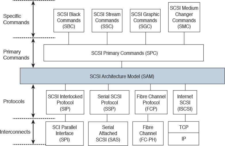
In the SCSI third-generation standard (SCSI-3), SAM defines SCSI commands (primary and specific for each peripheral) that are completely independent from the SCSI interconnects and their respective protocols, allowing an easy portability to other types of interconnects.
For example, Serial Attached SCSI (SAS) was specifically designed to overcome the limitations of the SCSI Parallel Interface. Defined as point-to-point serial connection, SAS can attach two devices through a maximum speed of 6 Gbps and over distances shorter than 10 meters (33 feet). This standard has achieved relative popularity with internal HDDs and, as SATA, is also commonly used on the back end of multiple disk array models.
In the mid-1990s, the Small Form Factor (SFF) committee introduced ATA Packet Interface (ATAPI), which extended PATA to other devices, such as CD-ROMs, DVDROMs, and tape drives. More importantly, ATAPI allowed an ATA physical connection to carry SCSI commands and data, serving as an alternative interconnect for this widespread standard. On the other hand, SAS offers compatibility with SATA disks through the SATA Tunneling Protocol (STP). Therefore, ATA commands can be carried over SCSI media (with STP) and vice versa (with ATAPI).
Another popular interconnect option is Fibre Channel (FC), which can be defined as a series of protocols that provides high-speed data communication between computer systems. Created in 1988, Fibre Channel has established itself as the main SAN protocol, providing block I/O access between servers and shared storage devices. Fibre Channel currently offers speeds of up to 16 Gbps, 10-km reach, and potentially millions of connected hosts in a single network.
Internet SCSI (iSCSI) is essentially a SAN technology that allows the transport of SCSI commands and data over a TCP connection. An iSCSI session can be directed to an iSCSI port on a storage array or a gateway between the iSCSI initiator and storage devices connected through other SAN protocols.
Both SAN technologies will be further explored in the following sections.
Fibre Channel Basics
Since its ratification in 1994 by the INCITS Technical Committee T11, Fibre Channel has become the most popular protocol for enterprise and service provider storage-area networks. Originally conceived to offer different types of data transport services to its connected nodes, Fibre Channel enables communication devices to form a special kind of network called fabric.
With speeds starting at 1 Gbps, Fibre Channel offers transport services to higher-level protocols such as SCSI, IBM’s Single-Byte Command Code Sets (SBCCS) for mainframe storage access, and the Internet Protocol (IP).
Like the majority of networking architectures, Fibre Channel does not follow the Open Systems Interconnection (OSI) model. Instead, it divides its protocols and functions into different hierarchical layers with predefined responsibilities, as described in Table 8-4 and exhibited in Figure 8-15.


Figure 8-15 represents how the following T11 standards fit into the Fibre Channel five-layer model:
![]() Fibre Channel Physical and Signaling Interface (FC-PH)
Fibre Channel Physical and Signaling Interface (FC-PH)
![]() Fibre Channel Physical Interface (FC-PI)
Fibre Channel Physical Interface (FC-PI)
![]() Fibre Channel Framing and Signaling (FC-FS)
Fibre Channel Framing and Signaling (FC-FS)
![]() Fibre Channel Generic Services (FC-GS)
Fibre Channel Generic Services (FC-GS)
![]() Fibre Channel Arbitrated Loop (FC-AL)
Fibre Channel Arbitrated Loop (FC-AL)
![]() Fibre Channel Fabric and Switch Control Requirements (FC-SW)
Fibre Channel Fabric and Switch Control Requirements (FC-SW)
![]() Fibre Channel Protocol for SCSI (SCSI-FCP)
Fibre Channel Protocol for SCSI (SCSI-FCP)
![]() FC Mapping for Single Byte Command Code Sets (FC-SB)
FC Mapping for Single Byte Command Code Sets (FC-SB)
![]() Transmission of IPv4 and ARP Packets over Fibre Channel (IPv4FC)
Transmission of IPv4 and ARP Packets over Fibre Channel (IPv4FC)
Tip
You can find much more detailed information about Fibre Channel standards at http://www.t11.org/t11/als.nsf/v2guestac.
Fibre Channel Topologies
Fibre Channel supports three types of topologies:
![]() Point-to-point: Connects two Fibre Channel–capable hosts without the use of a communication device, such as a Fibre Channel switch or hub. In this case, Fibre Channel is actually being used for a DAS connection.
Point-to-point: Connects two Fibre Channel–capable hosts without the use of a communication device, such as a Fibre Channel switch or hub. In this case, Fibre Channel is actually being used for a DAS connection.
![]() Arbitrated loop: Permits up to 127 devices to communicate with each other in a looped connection. Fibre Channel hubs were designed to improve reliability in these topologies, but with the higher adoption of switched fabrics, Fibre Channel loop interfaces are more likely to be found on legacy storage devices such as JBODs or older tape libraries.
Arbitrated loop: Permits up to 127 devices to communicate with each other in a looped connection. Fibre Channel hubs were designed to improve reliability in these topologies, but with the higher adoption of switched fabrics, Fibre Channel loop interfaces are more likely to be found on legacy storage devices such as JBODs or older tape libraries.
![]() Switched fabric: Comprises Fibre Channel devices that exchange data through Fibre Channel switches and theoretically supports up to 16 million devices in a single fabric.
Switched fabric: Comprises Fibre Channel devices that exchange data through Fibre Channel switches and theoretically supports up to 16 million devices in a single fabric.
Figure 8-16 illustrates these topologies, where each arrow represents a single fiber connection.

Figure 8-16 also introduces the following Fibre Channel port types:
![]() Node Port (N_Port): Interface on a Fibre Channel end host in a point-to-point or switched fabric topology.
Node Port (N_Port): Interface on a Fibre Channel end host in a point-to-point or switched fabric topology.
![]() Node Loop Port (NL_Port): Interface that is installed in a Fibre Channel end host to allow connections through an arbitrated loop topology.
Node Loop Port (NL_Port): Interface that is installed in a Fibre Channel end host to allow connections through an arbitrated loop topology.
![]() Fabric Port (F_Port): Interface Fibre Channel switch that is connected to an N_Port.
Fabric Port (F_Port): Interface Fibre Channel switch that is connected to an N_Port.
![]() Fabric Loop Port (FL_Port): Fibre Channel switch interface that is connected to a public loop. A fabric can have multiple FL_Ports connected to public loops, but, per definition, a private loop does not have a fabric connection.
Fabric Loop Port (FL_Port): Fibre Channel switch interface that is connected to a public loop. A fabric can have multiple FL_Ports connected to public loops, but, per definition, a private loop does not have a fabric connection.
![]() Expansion Port (E_Port): Interface that connects to another E_Port in order to create an Inter-Switch Link (ISL) between switches.
Expansion Port (E_Port): Interface that connects to another E_Port in order to create an Inter-Switch Link (ISL) between switches.
Fibre Channel Addresses
Fibre Channel uses two types of addresses to identify and locate devices in a switched fabric: World Wide Names (WWNs) and Fibre Channel Identifiers (FCIDs).
In theory, a WWN is a fixed 8-byte identifier that is unique per Fibre Channel entity. Following the format used in Cisco Fibre Channel devices, this writing depicts WWNs as colon-separated bytes (10:00:00:00:c9:76:fd:31, for example).
A Fibre Channel device can have multiple WWNs, where each address may represent a part of the device, such as:
![]() Port WWN (pWWN): Singles out one interface from a Fibre Channel node (or a Fibre Channel host bus adapter [HBA] port) and characterizes an N_Port
Port WWN (pWWN): Singles out one interface from a Fibre Channel node (or a Fibre Channel host bus adapter [HBA] port) and characterizes an N_Port
![]() Node WWN (nWWN): Represents the node (or HBA) that contains at least one port
Node WWN (nWWN): Represents the node (or HBA) that contains at least one port
![]() Switch WWN (sWWN): Uniquely represents a Fibre Channel switch
Switch WWN (sWWN): Uniquely represents a Fibre Channel switch
![]() Fabric WWN (fWWN): Identifies a switch Fibre Channel interface and distinguishes an F_Port
Fabric WWN (fWWN): Identifies a switch Fibre Channel interface and distinguishes an F_Port
Figure 8-17 displays how these different WWNs are assigned to distinct components of a duplicated host connection to a Fibre Channel switch.

In opposition, FCIDs are administratively assigned addresses that are inserted on Fibre Channel frame headers and represent the location of a Fibre Channel N_Port in a switched topology. An FCID consists of 3 bytes, which are detailed in Figure 8-18.

Each byte has a specific meaning in an FCID, as follows:
![]() Domain ID: Identifies the switch where this device is connected
Domain ID: Identifies the switch where this device is connected
![]() Area ID: May represent a subset of devices connected to a switch or all NL_Ports connected to an FL_Port
Area ID: May represent a subset of devices connected to a switch or all NL_Ports connected to an FL_Port
![]() Port ID: Uniquely characterizes a device within an area or domain ID
Port ID: Uniquely characterizes a device within an area or domain ID
To maintain consistency with Cisco MDS 9000 and Nexus switch commands, this writing describes FCIDs as contiguous hexadecimal bytes preceded by the “0x” symbol (0x01ab9e, for example).
At this point, you may be tempted to make mental associations between WWNs, FCIDs, MAC addresses, and IP addresses. Although it is a strong temptation, I advise you avoid the urge for now. Fibre Channel is easier to learn when you clear your mind about other protocol stacks.
Fibre Channel Flow Control
As part of a network architecture capable of providing lossless transport of data, a Fibre Channel device must determine whether there are enough resources to process a frame before receiving it. As a result, a flow control mechanism is needed to avoid frame discarding within a Fibre Channel fabric.
Fibre Channel deploys credit-based strategies to control data exchange between directly connected ports or between end nodes. In both scenarios, the receiving end is always in control, while the transmitter only sends a frame if it is sure that the receiver has available resources (buffers) to handle this frame.
Buffer-to-Buffer Credits (BB_Credits) are used to control frame transmission between directly connected ports (for example, N_Port to F_Port, N_Port to N_Port, or E_Port to E_Port). In essence, each port is aware of how many buffers are available to receive frames at the other end of the connection, only transmitting a frame if there is at least a single available buffer.
BB_Credit counters are usually configured with low two-digit values when both connected ports belong to the same data center. However, in data center interconnections over longer distances, a small number of BB_Credits may result in low performance. Such behavior can occur because the transmitting port sends as many frames as it can and then must wait for more BB_Credits from the receiving port to transmit again. The higher the latency on the interconnection, the longer the wait and the less traffic that traverses this link (regardless of its available bandwidth).
Distinctively, the End-to-End Credits (EE_Credits) flow control method regulates the transport of frames between source and destination N_Ports (such as an HBA and a disk array storage port). With a very similar mechanism to BB_Credits, this method allows a sender node to receive the delivery confirmation of frames from the receiver node.
Fibre Channel Processes
The Fibre Channel standards formally define a fabric as the “entity that interconnects various N_Ports attached to it and is capable of routing frames by using only the D_ID (destination domain ID) information in an FC-2 frame header.” The problem with this definition is that it does not really differentiate a fabric from a network.
However, as a recent trend, the networking industry has chosen the term fabric to represent a set of network devices that can somehow behave like one single device. And being the first architecture to use the term, Fibre Channel has influenced other networking technologies (including Ethernet) to also use the term as they embody characteristics from Fibre Channel such as simplicity, reliability, flexibility, minimum operation overhead, and support of new applications without disruption.
You will find a deeper discussion about Ethernet fabrics in Chapter 10, “Network Architectures for the Data Center: Unified Fabric,” and Chapter 11, “Network Architectures for the Data Center: SDN and ACI.”
Within Fibre Channel, many of these qualities are natively deployed through fabric services, which are basic functions that Fibre Channel end nodes can access through certain well-known FCID addresses, defined in the 0xfffff0 to 0xffffff range. Table 8-5 lists some of these fabric services and their respective well-known addresses.

The Broadcast Alias service can be accessed in a Fibre Channel switch when a frame is sent to address 0xffffff. Upon reception on this condition, a switch must replicate and transmit the frame to other active ports (according to a predefined broadcast policy).
The Login Server service is a fundamental service for N_Ports from each fabric switch that receives and responds to Fabric Login (FLOGI) frames. Such procedure is used to discover the operating characteristics associated with a fabric and its elements. Additionally, the Login Server service assigns the FCID for the requesting N_Port.
Tip
As you will see in the section “Fibre Channel Logins,” later in this chapter, T11 also defines other logins besides FLOGI.
The Fabric Controller service is the logical entity responsible for internal fabric operations such as
![]() Fabric initialization
Fabric initialization
![]() Parsing and routing of frames directed to well-known addresses
Parsing and routing of frames directed to well-known addresses
![]() Setup and teardown of ISLs
Setup and teardown of ISLs
![]() Frame routing
Frame routing
![]() Generation of fabric error responses
Generation of fabric error responses
The Name Server service stores information about active N_Ports, including their WWNs, FCIDs, and other Fibre Channel operating parameters (such as supported ULP). These values are commonly used to inform a node about FCID-pWWN associations in the fabric.
Finally, the Management Server service is an informative service that is used to collect and report information about link utilization, service errors, and so on.
Fabric Shortest Path First
A Fibre Channel switched fabric must be in an operational state to successfully transport frames between N_Ports. A key element called a principal switch is instrumental for this process, because it is responsible for domain ID distribution within the fabric.
The election of a principal switch depends on the priority assigned to each switch (1 to 254, where the lower value wins), and if a tie happens, it depends on each sWWN (lower wins again).
After the principal switch assigns domain IDs to all other switches in a fabric, routing tables start to be populated with entries that will be used to correctly route frames based on their destination domain ID and using the best available path.
Fibre Channel uses the Fabric Shortest Path First (FSPF) protocol to advertise domain IDs to other switches so that they can build their routing tables. As a link-state path selection protocol, FSPF keeps track of the state of the active links, associates a cost with each link, and finally calculates the path with the lowest cost between every two switches in the fabric.
By default, FSPF assigns the values 1000, 500, 250, 125, and 62 to 1-, 2-, 4-, 8-, and 16-Gbps links. But in Cisco Fibre Channel devices, you can also manually assign the cost of an ISL.
Conceived to clarify these theoretical concepts, Figure 8-19 illustrates how path costs are used to route Fibre Channel frames between N_Ports.

In Figure 8-19, a fabric is composed of three switches, named Switch1, Switch2, and Switch3. During the fabric initialization, Switch1 was elected principal switch and assigned to itself the domain ID 0x1a. Afterward, it assigned to Switch2 and Switch3 domain IDs 0x2b and 0x3c, respectively.
Using FSPF, the switches exchange routes based on their own domain ID and build routing tables, shown in Figure 8-19. Also noticeable is the fact that the Fibre Channel initiator (Server1) and targets (Storage2 and Storage3) have already received FCIDs during their FLOGI process, and that the first byte on these addresses corresponds to the domain ID of their directly connected switch.
Therefore, to route frames between two Fibre Channel N_Ports, each switch observes the destination domain ID in each frame, performs a lookup in its routing table, and sends the frame to the outgoing interface pointed to in the route entry. This process is repeated until the frame reaches the switch that is directly connected to the destination N_Port.
Tip
Figure 8-19 follows the interface naming process used in Cisco Fibre Channel switches, where the first number refers to the slot order and the second to the order of the interface in a module.
Notice in Figure 8-19 that there are two paths with an FSPF cost of 250 between Switch1 and Switch3. Thus, the frame sent from Server1 to Storage3 (represented in a very simplified format) may be forwarded to one of two interfaces on Switch1: fc1/1 or fc2/2.
According to the Fibre Channel standards, it is up to each manufacturer to decide how a switch forwards frames in the case of equal-cost paths. Cisco Fibre Channel switches can load-balance traffic on up to 16 equal-cost paths using one of the following behaviors:
![]() Flow-based: Each pair of N_Ports only uses a single path (for example, traffic from Server1 to Storage3 will only use the path Switch1–Switch3). The path choice is based on a hash function over the source and destination FCIDs of each frame.
Flow-based: Each pair of N_Ports only uses a single path (for example, traffic from Server1 to Storage3 will only use the path Switch1–Switch3). The path choice is based on a hash function over the source and destination FCIDs of each frame.
Tip
A hash function is an operation that can map digital data of any size to digital data of fixed size. In the case of FSPF load-balancing, a hash function of the same arguments (destination and source FCIDs) will always result in the same path among all equal-cost shortest paths.
![]() Exchange-based: Exchanges from each pair of N_Ports are load-balanced among all available paths. The path choice is based on a hash operation over the source and destination FCIDs of each frame, plus a Fibre Channel header called Originator Exchange Identifier (OX_ID), which is unique for each SCSI I/O operation (read or write).
Exchange-based: Exchanges from each pair of N_Ports are load-balanced among all available paths. The path choice is based on a hash operation over the source and destination FCIDs of each frame, plus a Fibre Channel header called Originator Exchange Identifier (OX_ID), which is unique for each SCSI I/O operation (read or write).
Because FSPF does not take into account the available bandwidth or utilization of the paths for route calculation, SAN administrators must carefully plan FSPF to consider failure scenarios and to avoid traffic bottlenecks.
Unlike the topology shown in Figure 8-19, SAN administrators commonly deploy ISL redundancy between switches. However, these professionals still need to be aware that if an ISL changes its operational state, a general route recomputation can bring instability and traffic loss to a fabric.
To reduce these risks, using PortChannels is highly recommended because they can aggregate multiple ISLs into one logical connection (from the FSPF perspective).
Figure 8-20 compares how a fabric with nonaggregated ISLs and a fabric with PortChannels behave after a link failure.

When PortChannels are not being deployed, a link failure will always cause route recomputation because a link state has changed for FSPF. In the fabric depicted on the right in Figure 8-20, such a failure is confined to the logical ISL (the PortChannel itself), not causing any FSPF change in the fabric if at least one PortChannel member is operational.
In a nutshell, PortChannels increase the reliability of a Fibre Channel fabric and simplify its operation, reducing the number of available FSPF paths between switches.
Fibre Channel Logins
A Fibre Channel N_Port carries out three basic login processes before it can properly exchange frames with another N_Port in a switched fabric. These login processes are described in Table 8-6.

Figure 8-21 exhibits a FLOGI process between a server HBA and Switch1, and another between an array storage port and Switch2. Afterward, each N_Port receives an FCID that is inserted into a FLOGI database located in its directly connected switch. Both switches will use this table to forward Fibre Channel frames to local ports.

Figure 8-21 also shows subsequent PLOGI and PRLI processes between the same HBA and a storage array port. After all these negotiations, both devices are ready to proceed with their upper-layer protocol communication using Fibre Channel frames.
Zoning
A zone is defined as a subset of N_Ports from a fabric that are aware of each other, but not of devices outside the zone. Each zone member can be specified by a port on a switch, WWN, FCID, or human-readable alias (also known as FC-Alias).
Zones are configured in Fibre Channel switched fabrics to increase network security, introduce storage access control, and prevent data loss. By using zones, a SAN administrator can avoid a scenario where multiple servers can access the same storage resource, ruining the stored data for all of them.
A fabric can deploy two methods of zoning:
![]() Soft zoning: Zone members are made visible to each other through name server queries. With this method, unauthorized frames are capable of traversing the fabric.
Soft zoning: Zone members are made visible to each other through name server queries. With this method, unauthorized frames are capable of traversing the fabric.
![]() Hard zoning: Frame permission and blockage is enforced as a hardware function on the fabric, which in turn will only forward frames among members of a zone. Cisco Fibre Channel switches only deploy this method.
Hard zoning: Frame permission and blockage is enforced as a hardware function on the fabric, which in turn will only forward frames among members of a zone. Cisco Fibre Channel switches only deploy this method.
Tip
In Cisco devices, you can also configure the switch behavior to handle traffic between unzoned members. To avoid unauthorized storage access, blocking is the recommended default behavior for N_Ports that do not belong to any zone.
A zone set consists of a group of one or more zones that can be activated or deactivated with a single operation. Although a fabric can store multiple zone sets, only one can be active at a time. The active zone set is present in all switches on a fabric, and only after a zone set is successfully activated can the N_Ports contained in each member zone perform PLOGIs and PRLIs between them.
Note
The Zone Server service is used to manage zones and zone sets. Implicitly, an active zone set includes all the well-known addresses from Table 8-5 in every zone.
Figure 8-22 illustrates how zones and an active zone set can be represented in a Fibre Channel fabric.

Although each zone in Figure 8-22 (A, B, and C) contains two or three members, more hosts could be inserted in them. When performing a name service query (“dear fabric, whom can I communicate with?”), each device receives the FCID addresses from members in the same zone and begins subsequent processes, such as PLOGI and PRLI.
Additionally, Figure 8-22 displays the following self-explanatory types of zones:
![]() Single-initiator, single-target (Zone A)
Single-initiator, single-target (Zone A)
![]() Multi-initiator, single-target (Zone B)
Multi-initiator, single-target (Zone B)
![]() Single-initiator, multi-target (Zone C)
Single-initiator, multi-target (Zone C)
Tip
Because not all members within a zone should communicate, single-initiator, single-target zones are considered best practice in Fibre Channel SANs.
SAN Designs
In real-world SAN designs, it is very typical to deploy two isolated physical fabrics with servers and storage devices connecting at least one N_Port to each fabric. Undoubtedly, such best practice increases storage access availability (because there are two independent paths between each server and a storage device) and bandwidth (if multipath I/O software is installed on the servers, they may use both fabrics simultaneously to access a single storage device).
There are, of course, some exceptions to this practice. In many data centers, I have seen backup SANs with only one fabric being used for the connection between dedicated HBA ports in each server, tape libraries, and other backup-related devices.
Another key aspect of SAN design is oversubscription, which generically defines the ratio between the maximum potential consumption of a resource and the actual resource allocated in a communication system. In the specific case of Fibre Channel fabrics, oversubscription is naturally derived from the comparison between the number of HBAs and storage ports in a single fabric.
Because storage ports are essentially a shared resource among multiple servers (which rarely use all available bandwidth in their HBAs), the large majority of SAN topologies are expected to present some level of oversubscription. The only completely nonoversubscribed SAN topology is DAS, where every initiator HBA port has its own dedicated target port.
In classic SAN designs, an expected oversubscription between initiators and targets must be obeyed when deciding how many ports will be dedicated for HBAs, storage ports, and ISLs. Typically, these designs use oversubscriptions from 4:1 (four HBAs for each storage port, if they share the same speed) to 8:1.
Tip
Such expected oversubscription is also known as fan-out.
With these concepts in mind, we will explore three common SAN topologies, which are depicted in Figure 8-23.

The left side of Figure 8-23 represents the single-layer topology, where only one Fibre Channel switch is positioned between the server HBAs and the storage ports on disk arrays. The simplicity of this topology also limits its scalability to the maximum number of ports of a single Fibre Channel switch. For this reason, positioning Fibre Channel director-class switches (or simply, directors) in this topology is usually better, because they can offer a larger number of ports when compared to fabric switches, as well as high availability on all of their internal components. This topology is also known as collapsed-core as a direct result of the highly popular process in the 2000s of consolidating multiple fabric switches into directors.
Note
You will find more details about Cisco MDS 9000 fabric switches and directors in Chapter 13, “Cisco Cloud Infrastructure Portfolio.”
The center topology in Figure 8-23 depicts a very traditional topology called core-edge, where two layers of communication devices are positioned between initiators and targets. In this case, each layer is dedicated to the connection of a single type of device (servers on edge and storage devices on core). In core-edge topologies, the number of ISLs between both layers is defined according to the SAN expected oversubscription and available port speeds.
Also in core-edge designs, the number of ports on edge devices depends on the type of physical connection arrangement to the servers. In top-of-rack connections, where the servers share the same rack with their access devices, fabric switches with less than 48 Fibre Channel ports are usually deployed. If end-of-row connections are used, directors are commonly positioned to offer connection access to servers distributed across many racks.
Finally, the topology on the right in Figure 8-23 depicts the edge-core-edge topology, which is deployed in SANs that require thousands of ports in a single physical structure. In an edge-core-edge fabric, there are two kinds of edge switches: target edges and initiator edges. These switches are used, respectively, to connect to storage devices and to connect to servers. All traffic coalesces in the core switches, whose number of devices and deployed ISLs controls the SAN oversubscription.
As a way to transcend some scalability limits on Fibre Channel SANs, such as the number of domain IDs in a single fabric, it is possible to deploy a virtualization technique called N_Port Virtualization (NPV). Running in NPV mode, a switch can emulate an N_Port connected to an upstream switch F_Port, which eliminates the need to deploy an ISL and the insertion of an additional domain ID in the fabric.
Figure 8-24 details the differences between a standard ISL and an NPV connection.
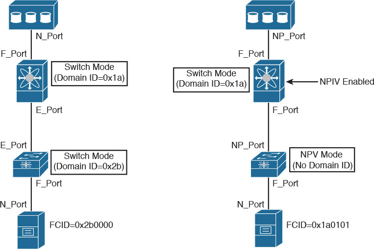
Unlike a standard Fibre Channel switch, a switch in NPV mode performs a fabric login (FLOGI) in an upstream switch through a Node Proxy Port (NP_Port), which receives an FCID in the upstream switch in response. Afterward, the NPV-mode switch uses this NP_Port to forward all FLOGIs from connected servers to the upstream switch. Figure 8-24 also highlights that the host connected to the NPV-mode switch received FCID 0x1a0101, which is derived from the core switch domain ID.
Finally, an NPV connection requires that an upstream F_Port can receive and process more than one fabric login. To support such behavior, the upstream switch must deploy a capability called N_Port ID Virtualization (NPIV).
Virtual SANs
Until the late 1990s, storage administrators deployed SAN islands to avoid fabric-wide disruptive events from one application environment causing problems in other environments. Their concept was really simple: independent and relatively small fabrics that connect servers and storage dedicated to a single application.
When storage administrators needed more ports, they typically scaled these SAN islands through the connection of small fabric switches. With time, the deployment of SAN islands produced some architectural challenges, such as
![]() Low utilization of storage resources that were connected to a single island
Low utilization of storage resources that were connected to a single island
![]() Large number of management points
Large number of management points
![]() Considerable number of ports used for ISLs
Considerable number of ports used for ISLs
![]() Unpredictable traffic oversubscription on ISLs
Unpredictable traffic oversubscription on ISLs
In the next decade, a significant number of data centers started SAN consolidation projects to eliminate these undesirable effects. And as I mentioned in the section “SAN Designs,” director-class switches were ideal tools for these projects.
To avoid the formation of a single failure domain in a consolidated physical fabric, Cisco introduced the concept of virtual storage-area networks (VSANs). Supporting the creation of virtual SAN islands, VSANs can bring several other advantages to SAN administrators, as you will learn in the following sections.
VSAN Definitions
A VSAN is defined as a set of N_Ports that share the same Fibre Channel fabric processes in a single physical SAN. As a consequence, all fabric services such as Name Server, Zone Server, and Login Server present distinct instances per VSAN.
In Cisco devices, VSAN Manager is the network operating system process that maintains VSAN attributes and port membership. It employs a database that contains information about each VSAN, such as its unique name, administrative state (suspended or active), operational state (up, if the VSAN has at least one active interface), load-balance algorithm (for FSPF equal-cost paths and PortChannels), and Fibre Channel timers.
In a VSAN-capable device, there are two predefined virtual SANs:
![]() Default (VSAN 1): This VSAN cannot be erased, only suspended. It contains all the ports when a switch is first initialized.
Default (VSAN 1): This VSAN cannot be erased, only suspended. It contains all the ports when a switch is first initialized.
![]() Isolated (VSAN 4094): This special VSAN receives all the ports from deleted VSANs and, per definition, does not forward any traffic. It exists to avoid involuntary inclusion of ports in a VSAN and it cannot be deleted either.
Isolated (VSAN 4094): This special VSAN receives all the ports from deleted VSANs and, per definition, does not forward any traffic. It exists to avoid involuntary inclusion of ports in a VSAN and it cannot be deleted either.
An example usually is clearer than a theoretical explanation, so to illustrate how VSANs behave, Figure 8-25 depicts a single MDS 9000 switch (MDS1) deploying two different VSANs. Observe that among the four interfaces, VSAN 100 contains interfaces fc1/1 and fc2/1, while VSAN 200 contains fc1/2 and fc1/3.

Example 8-1 explains how both VSANs were created on switch MDS1 as well as the interface assignment configuration.
Example 8-1 VSAN Creation and Interface Assignment
! Entering the configuration mode
MDS1# configure terminal
! Entering the VSAN configuration database
MDS1(config)# vsan database
! Creating VSAN 100
MDS1(config-vsan-db)# vsan 100
! Including interfaces fc1/1 and fc2/1 in VSAN 10, one at a time
MDS1(config-vsan-db)# vsan 100 interface fc1/1
MDS1(config-vsan-db)# vsan 100 interface fc2/1
! Creating VSAN 200
MDS1(config-vsan-db)# vsan 200
! Both interfaces fc1/2 and fc1/3 are included in VSAN 20
MDS1(config-vsan-db)# vsan 200 interface fc1/2-3
! Now, all interfaces are simultaneously enabled
MDS1(config-vsan-db)# interface fc1/1-3,fc2/1
MDS1(config-if)# no shutdown
If all interfaces on MDS1 are configured in automatic mode, it is expected that all four devices will perform their FLOGI into both VSANs. Example 8-2 proves this theory.
Example 8-2 FLOGI Database in MDS1
! Displaying the flogi database
MDS1(config-if)# show flogi database
--------------------------------------------------------------------------------
INTERFACE VSAN FCID PORT NAME NODE NAME
--------------------------------------------------------------------------------
! Server1 is connected to domain ID 0xd4
fc1/1 100 0xd40000 10:00:00:00:c9:2e:66:00 20:00:00:00:c9:2e:66:00
! Server2 and Storage2 are connected to domain ID 0xed
fc1/2 200 0xed0000 10:00:00:04:cf:92:8b:ad 20:00:00:04:cf:92:8b:ad
fc1/3 200 0xed00dc 22:00:00:0c:50:49:4e:d8 20:00:00:0c:50:49:4e:d8
! Storage1 is connected to domain ID 0xd4
fc2/1 100 0xd400da 50:00:40:21:03:fc:6d:28 20:03:00:04:02:fc:6d:28
In Example 8-2, VSANs 100 and 200 have different domain IDs (0xd4 and 0xed, respectively) that were randomly chosen from the domain ID list (1 to 239, by default) in each VSAN. Additionally, the VSAN distinct Login Servers have, accordingly, assigned FCIDs to the connected storage devices. As a result, MDS1 has created two virtual SAN islands. And from their own perspective, each initiator-target pair is connected to completely different switches.
VSAN Trunking
Just like their physical counterparts, VSANs are usually not created to be restricted to a single switch. In fact, they can be extended to other switches from core-edge or edge-core-edge topologies, for example. Although ISLs could potentially be configured to transport frames from a single VSAN, to avoid waste of ports, a trunk is usually the recommended connection between VSAN-enabled switches.
By definition, a Trunk Expansion Port (TE_Port) can carry the traffic of several VSANs over a single Enhanced Inter-Switch Link (EISL). In all frames traversing these special ISLs, an 8-byte VSAN header is included before the frame header. Although this header structure is not depicted here, you should know that it includes a 12-bit field that identifies the VSAN each frame belongs to.
Note
The VSAN header is standardized in FC-FS-2 section 10.3 (“VFT_Header and Virtual Fabrics”).
Figure 8-26 illustrates an EISL configured between two switches (MDS-A and MDS-B). It also depicts the interface configuration used on both devices.

In the figure, the switchport command is first used to configure the port type (E_Port), then to enable VSAN trunking, and then to allow VSANs 10 and 20 to use the trunk on both switches. Consequently, an EISL is formed, causing frames (also portrayed in Figure 8-26) from intra-VSAN traffic to be tagged in this special connection.
Zoning and VSANs
Two steps are usually executed to present a SCSI storage volume (LUN) from a disk array to a server. Therefore, after both of them are logged to a common Fibre Channel fabric:
Step 1. Both device ports must be zoned together.
Step 2. In the storage array, the LUN must be configured to be solely accessed by a pWWN from the server port. This process is commonly referred as LUN masking.
When deploying VSANs, a SAN administrator performs these activities as if she were managing different Fibre Channel fabrics. Hence, each VSAN has its own zones and zone sets (active or not).
Still referring to the topology from Figure 8-26, Example 8-3 details a zoning configuration that permits Server10 (whose HBA has pWWN 10:00:00:00:c9:2e:66:00) to communicate with Array10 (whose port has pWWN 50:00:40:21:03:fc:6d:28) after VSANs 10 and 20 are already provisioned.
Example 8-3 Zoning Server10 and Array10 on MDS-A
! Creating a zone in VSAN 10
MDS-A(config)# zone name SERVER10-ARRAY10 vsan 10
! Including Server10 pWWN in the zone
MDS-A(config-zone)# member pwwn 10:00:00:00:c9:2e:66:00
! Including Array10 pWWN in the zone
MDS-A(config-zone)# member pwwn 50:00:40:21:03:fc:6d:28
! Creating a zone set and including zone SERVER10-ARRAY10 in it
MDS-A(config-zone)# zoneset name ZS10 vsan 10
MDS-A(config-zoneset)# member SERVER10-ARRAY10
! Activating the zone set
MDS-A(config-zoneset)# zoneset activate name ZS10 vsan 10
Zoneset activation initiated. check zone status
! At this moment, all switches in VSAN 10 share the same active zone set
MDS-A(config)# show zoneset active vsan 10
zoneset name ZS10 vsan 10
zone name SERVER10-ARRAY10 vsan 10
* fcid 0x710000 [pwwn 10:00:00:00:c9:2e:66:00]
* fcid 0xd40000 [pwwn 50:00:40:21:03:fc:6d:28]
Tip
Because the zone service is a distributed fabric process, I could have chosen either of the switches for this configuration.
In Example 8-3, I have chosen pWWNs to characterize both devices in the zone because these values will remain the same, wherever they are connected in the fabric. Nevertheless, other methods can be used to include a device in a zone, such as switch interface and FCID.
The stars on the side of each zone member signal that these nodes are logged in and present in the VSAN 10 fabric. At the end of Example 8-3, they are zoned together.
Figure 8-27 exhibits the 20-GB disk array volume detected on Server10, which uses Windows 2008 as its operating system. From this moment on, Server10 can store data on this volume through standard SCSI commands.

In Example 8-4, it is possible to verify that the Zone Server on VSAN 20 is completely unaware of the recent zone set activated in VSAN 10.
Example 8-4 Displaying Active Zone Set in VSAN20
MDS-A(config)# show zoneset active vsan 20
Zoneset not present
MDS-A(config)#
VSAN Use Cases
I usually recommend the creation of an additional VSAN whenever a SAN administrator feels the sudden urge to deploy another physical Fibre Channel fabric in his environment. Following this train of thought, VSANs can be effectively deployed to achieve the following:
![]() Consolidation: As previously mentioned, VSANs originally allowed many SAN islands to be put together within the same physical infrastructure.
Consolidation: As previously mentioned, VSANs originally allowed many SAN islands to be put together within the same physical infrastructure.
![]() Isolation: A VSAN basically creates an additional Fibre Channel fabric that does not interfere with environments that already exist. As a way to avoid investment in additional SAN switches, VSANs can be easily applied to support development, qualification, and production environments for the same application.
Isolation: A VSAN basically creates an additional Fibre Channel fabric that does not interfere with environments that already exist. As a way to avoid investment in additional SAN switches, VSANs can be easily applied to support development, qualification, and production environments for the same application.
![]() Multi-tenancy: Virtual SANs can easily build, on a shared infrastructure, separate fabric services and traffic segmentation for servers and storage devices that belong to different companies. Moreover, the management of all VSAN resources can be assigned to distinct tenant administrators through the use of Role-based Access Control (RBAC) features.
Multi-tenancy: Virtual SANs can easily build, on a shared infrastructure, separate fabric services and traffic segmentation for servers and storage devices that belong to different companies. Moreover, the management of all VSAN resources can be assigned to distinct tenant administrators through the use of Role-based Access Control (RBAC) features.
![]() Interoperability: As one of the first Cisco innovations brought to a hardly open industry, MDS 9000 interoperability features enabled the integration of third-party switches through the use of additional VSANs. In essence, a VSAN in interoperability mode emulates all the characteristics of a third-party device without compromising other environments.
Interoperability: As one of the first Cisco innovations brought to a hardly open industry, MDS 9000 interoperability features enabled the integration of third-party switches through the use of additional VSANs. In essence, a VSAN in interoperability mode emulates all the characteristics of a third-party device without compromising other environments.
Note
A feature called Inter-VSAN Routing (IVR) can be used whenever two devices that belong to different VSANs must communicate with each other. In migration scenarios that use VSANs in interoperability mode, IVR is heavily used.
Certainly, this list is not an exhaustive exploration of VSAN applicability, as many more use cases were created to support specific requirements of many other customers. But fundamentally, this virtualization technique drastically decreased SAN provisioning time as well as the number of unused ports during the endemic formation of physical SAN “archipelagos” in the 1990s.
Internet SCSI
A joint initiative between Cisco and IBM, Internet SCSI (or simply iSCSI) was originally intended to port SCSI peripherals into the flourishing IP networks. Fostering convergence over a single network infrastructure, iSCSI connections can leverage an existent local-area network (LAN) (and potentially wide-area networks [WANs]) to establish block-based communications between servers and storage devices.
Standardized in the IETF RFC 3720 in 2004, iSCSI employs TCP connections to encapsulate SCSI traffic (and perform flow control). For that reason, iSCSI has consequently achieved great popularity as a quick-to-deploy alternative SAN technology.
As depicted in Figure 8-28, the main components of the iSCSI architecture are
![]() iSCSI initiator: Server that originates an iSCSI connection to an iSCSI portal identified by an IP address and a TCP destination port (default is 3260). An initiator usually employs a software client to establish a session and (optionally) an offload engine to unburden the CPU of the overhead associated with iSCSI or TCP processing. However, as computer processor speeds continue to abide by Moore’s law, the great majority of iSCSI implementations still rely on idle resources from the CPU and forego the optional offload engine.
iSCSI initiator: Server that originates an iSCSI connection to an iSCSI portal identified by an IP address and a TCP destination port (default is 3260). An initiator usually employs a software client to establish a session and (optionally) an offload engine to unburden the CPU of the overhead associated with iSCSI or TCP processing. However, as computer processor speeds continue to abide by Moore’s law, the great majority of iSCSI implementations still rely on idle resources from the CPU and forego the optional offload engine.
Fibre Channel HBAs relieve the server processor from all overhead related to SCSI and Fibre Channel communication.
![]() iSCSI target: Storage device that provides LUN access through iSCSI. Generally speaking, these targets establish an iSCSI portal to which multiple iSCSI initiators may connect.
iSCSI target: Storage device that provides LUN access through iSCSI. Generally speaking, these targets establish an iSCSI portal to which multiple iSCSI initiators may connect.
![]() iSCSI gateway: Communication device that allows the communication between iSCSI initiators and targets connected to different SAN technologies. Select MDS 9000 switches and directors are capable of establishing portals for iSCSI initiators and initiators for Fibre Channel storage devices.
iSCSI gateway: Communication device that allows the communication between iSCSI initiators and targets connected to different SAN technologies. Select MDS 9000 switches and directors are capable of establishing portals for iSCSI initiators and initiators for Fibre Channel storage devices.

Note
Over the years, I have witnessed many discussions regarding the question of whether iSCSI requires a separate IP network. Excluding political and governance arguments, I would say that iSCSI traffic can be easily protected in modern data center networks through familiar network technologies such as VLANs and Quality of Service (QoS). In such scenarios, I would recommend having an exclusive VLAN connecting dedicated iSCSI interfaces for both initiators and targets as a best practice, for two reasons: iSCSI initiators will not require additional host routes, and iSCSI traffic will be easily identified, by VLAN or IP subnet, for QoS purposes.
As an alternative to using IP addresses, devices at the end of an iSCSI connection can identify each other through specially defined naming schemes. The most commonly used structure is called an iSCSI Qualified Name (IQN), which may have up to 255 bytes and is formed with the concatenation of the following elements:
![]() Literal IQN: The prefix “iqn”
Literal IQN: The prefix “iqn”
![]() Date: The year and month
Date: The year and month
![]() Reverse domain name: Where “company.com” becomes “com.company”
Reverse domain name: Where “company.com” becomes “com.company”
![]() Optional colon and specific device name:
Optional colon and specific device name:
An example IQN name is “iqn.1993-11.com.disk-vendor:diskarrays.sn.45678.” If the iSCSI connection is using IQN-based authentication, the other host at the end of the connections must identify this exact string. Other, less common naming conventions for iSCSI are IEEE Extended Unique Identifier (EUI) and T11 Network Address Authority (NAA).
Designed as an additional service for large iSCSI deployments, Internet Storage Name Service (iSNS) enables automated discovery, management, and configuration of iSCSI devices. For this reason, iSNS is frequently compared to native Fibre Channel services such as Login Server and Name Server.
Although iSNS was standardized in 2005, the great majority of iSCSI implementations still depend on static portal definitions on initiators to establish iSCSI connections. As a consequence, iSCSI devices leverage high-availability mechanisms from both SCSI and IP protocols. For example:
![]() Multipathing: Ideally, each initiator and target pair deploys more than one interface to establish two independent iSCSI connections between these entities. With such arrangement, an initiator software client may choose to forward iSCSI traffic to only one connection or load-balance storage access between them. In both cases, if a session fails for any reason, the remaining connection maintains LUN access to the iSCSI initiator.
Multipathing: Ideally, each initiator and target pair deploys more than one interface to establish two independent iSCSI connections between these entities. With such arrangement, an initiator software client may choose to forward iSCSI traffic to only one connection or load-balance storage access between them. In both cases, if a session fails for any reason, the remaining connection maintains LUN access to the iSCSI initiator.
![]() Virtual Router Redundancy Protocol (VRRP): This protocol can provide high availability for iSCSI portals created on multiple target (or gateway) ports. In these scenarios, iSCSI initiators connect to a virtual IP address that is dynamically assigned to an interface deploying an iSCSI portal. In the case of a device (or port) failure, this special IP address is quickly reassigned to another device (or interface) and the iSCSI connection is reinitialized.
Virtual Router Redundancy Protocol (VRRP): This protocol can provide high availability for iSCSI portals created on multiple target (or gateway) ports. In these scenarios, iSCSI initiators connect to a virtual IP address that is dynamically assigned to an interface deploying an iSCSI portal. In the case of a device (or port) failure, this special IP address is quickly reassigned to another device (or interface) and the iSCSI connection is reinitialized.
iSCSI initiators, targets, and gateways can also leverage security mechanisms from both IP and SCSI architectures, including access control lists (ACLs) and LUN masking for specific IP addresses, subnets, or IQNs. RFC 3720 additionally predicted exclusive security measures for iSCSI, such as initiator identification through Challenge-Handshake Authentication Protocol (CHAP) and packet protection through Internet Protocol Security (IPSec).
Cloud Computing and SANs
As specialized environments built over standard data centers, cloud computing can certainly enjoy the same benefits from block-based storage and SANs. As you have learned in this chapter, these technologies greatly facilitate data portability because they obscure any distinction between local hard disk drives and remote volumes, while leveraging all advantages from modern disk arrays.
Fundamentally, block storage technologies can serve two objectives in cloud computing scenarios:
![]() Infrastructure: Where disk arrays and SAN devices are used to provide remote storage access to the systems supporting the cloud
Infrastructure: Where disk arrays and SAN devices are used to provide remote storage access to the systems supporting the cloud
![]() Block Storage as a Service: Where volumes are offered as cloud tenant resources
Block Storage as a Service: Where volumes are offered as cloud tenant resources
This section explores each of these possibilities using concepts and technologies you are already familiar with.
Block Storage for Cloud Infrastructure
Primarily, a data center architect usually includes SAN deployments in a project to establish a transparent decoupling between application software and the data it accesses. Such an approach greatly facilitates the replication of data and volume scaling up without unnecessary hardware changes in the application servers.
Considering the specific requirements of a cloud computing infrastructure, SANs can offer additional interesting functions such as
![]() SAN boot: Rather than using an internal HDD, a server can boot its operating system using a LUN on a remote storage device, simplifying hardware replacement if a critical component suffers any major malfunction. SAN boot is also a necessary step for the concept of stateless computing, where all server configurations (states) are not contained in the computer system. In this style of computing, a server is used exclusively as a processing resource.
SAN boot: Rather than using an internal HDD, a server can boot its operating system using a LUN on a remote storage device, simplifying hardware replacement if a critical component suffers any major malfunction. SAN boot is also a necessary step for the concept of stateless computing, where all server configurations (states) are not contained in the computer system. In this style of computing, a server is used exclusively as a processing resource.
![]() Cluster storage: Computer clusters are composed of multiple server nodes controlled by cluster software and performing identical tasks to achieve high availability and, in some cases, higher performance. Most cluster technologies require that the multiple nodes access the same data set simultaneously, which can be easily achieved in SAN deployments.
Cluster storage: Computer clusters are composed of multiple server nodes controlled by cluster software and performing identical tasks to achieve high availability and, in some cases, higher performance. Most cluster technologies require that the multiple nodes access the same data set simultaneously, which can be easily achieved in SAN deployments.
![]() Virtual machine datastores: Multiple virtualization hosts that run Type-1 hypervisors have access to the same volume storing VM files, thereby enabling server virtualization features such as VM high availability and live migration. This implementation can be considered a specific, but extremely popular, subtype of cluster storage.
Virtual machine datastores: Multiple virtualization hosts that run Type-1 hypervisors have access to the same volume storing VM files, thereby enabling server virtualization features such as VM high availability and live migration. This implementation can be considered a specific, but extremely popular, subtype of cluster storage.
Note
Most hypervisor architectures can perform VM storage live migration, which essentially allows the transfer of all files from virtual machines between two VM datastores without any loss of service.
Block Storage as a Service
Besides consuming block-based storage for its own structural purposes, there is no technical reason why a cloud computing environment cannot also provide these resources to end users. Therefore, through a Block Storage as a Service offering, a cloud tenant can request a volume to store data from applications deployed inside a cloud, or even to store data for external systems.
For public clouds, providing external access to automatically generated SCSI LUNs may be especially challenging due to the expected high latency of the Internet. Nevertheless, these volumes could potentially be provisioned for external servers that are sharing the same Fibre Channel SAN or Ethernet LAN (for iSCSI) with a private cloud.
In real-world scenarios, the most common Block Storage as a Service offerings today exist to create and attach volumes to Infrastructure as a Service (IaaS)-generated virtual machines. Several public cloud providers include this service in their portals, including Amazon Web Services through its Amazon Elastic Block Storage (EBS) and Microsoft Azure via its Azure Blob Storage.
OpenStack also offers a highly available component for Block Storage as a Service, named Cinder. Much like the services cited in the previous paragraph, Cinder is designed to allow Nova-instantiated virtual machines to access volumes dynamically provisioned on traditional block storage devices.
As explained, you should not consider Cinder as storage device emulation, simply because this OpenStack service does not actually receive or send application data directly from or to tenant VMs. In fact, Cinder provides an abstraction service that uses back-end storage drivers that enable several vendors to be controlled by an OpenStack cloud. In summary, OpenStack Cinder
![]() Provides a volume to a single VM instance
Provides a volume to a single VM instance
![]() Has an API to receive predefined end-user requests such as create volume and attach volume working in tandem with OpenStack Nova
Has an API to receive predefined end-user requests such as create volume and attach volume working in tandem with OpenStack Nova
![]() Selects the most appropriate storage device to deploy a volume
Selects the most appropriate storage device to deploy a volume
![]() Sends requests to the underlying storage systems to create and manage volumes
Sends requests to the underlying storage systems to create and manage volumes
![]() Sends storage information (using iSCSI credentials) to Nova for session establishment
Sends storage information (using iSCSI credentials) to Nova for session establishment
As a general comment, iSCSI is usually considered a better fit for Block Storage as a Service scenarios due to its flexibility of using software initiators in the virtual machines (as well as the amazing ubiquity of IP).
Around the Corner: Solid-State Drives
It is not exactly news that hard disk drives are not the only available technology for secondary storage functions, especially if you observe the huge gap of data access latency between main memory (30 to 60 nanoseconds) and HDDs (3,000,000 to 12,000,000 nanoseconds). And although that difference may be imperceptible to humans (the blink of an eye is on average 100,000,000 to 150,000,000 nanoseconds), it is certainly not for computers, where a single user request for a stored object may generate millions of individual I/O operations.
Dodging the electromechanical-related latencies of HDDs, solid-state drives (SSDs) were created several decades ago to better bridge the gap between primary and secondary storage, offering an access latency of less than 100 microseconds. SSDs share their origins with the widely popular USB flash drives, both being composed of the same integrated circuit assemblies that can persistently store data through power outages. For that reason, SSDs are also referred as flash drives by some vendors.
Perhaps to appeal to long-term HDD users, some vendors chose to market their SSD technology as “solid-state disk.” Regardless of the motivation, this technical misstep is not totally without merit, because most SSDs share compatible interfaces with HDDs. Employing SATA and SAS connections, SSDs can easily replace other technologies in personal computers, servers, and disk arrays.
Besides providing lower latency, SSDs are also more resistant to physical shock, produce less noise, and consume less power when compared to HDDs. And as the price difference with HDDs decreases, SSDs are increasingly becoming popular in application environments that require superior I/O performance. And once more, Cisco innovates modern data center architectures by positioning SSDs as part of the Unified Computing System (UCS) with UCS Invicta.
Fundamentally, UCS Invicta consists of an SSD-only storage system that is especially built to bring faster I/O operations through unique features. For this reason, it is primarily designed to accelerate applications such as database, email, virtual desktop, high-performance computing (HPC), and video transcoding applications.
UCS Invicta is available in two physical factors:
![]() Appliance: A single hardware piece that can be easily added to a UCS domain composed of blade or rack servers. It provides block I/O access to SCSI LUNs through Fibre Channel or iSCSI.
Appliance: A single hardware piece that can be easily added to a UCS domain composed of blade or rack servers. It provides block I/O access to SCSI LUNs through Fibre Channel or iSCSI.
![]() Scaling System: Composed of router nodes (which are responsible for connectivity and management, including replication, striping, and RAID configurations) and nodes deploying individual flash-memory management, including RAID and data protection.
Scaling System: Composed of router nodes (which are responsible for connectivity and management, including replication, striping, and RAID configurations) and nodes deploying individual flash-memory management, including RAID and data protection.
UCS Invicta OS is the storage operating system that controls both formats, providing the advanced features described in Table 8-7.

Note
Cisco has announced the end-of-sale for UCS Invicta solutions in 2015. However, I have maintained its content in this certification guide to address the CLDFND exam blueprint. You can find more details related to the product (such as capacity and scalability) in Chapter 13.
Further Reading
Exam Preparation Tasks
Review All the Key Topics
Review the most important topics in this chapter, denoted with a Key Topic icon in the outer margin of the page. Table 8-8 lists a reference of these key topics and the page number on which each is found.
Table 8-8 Key Topics for Chapter 8
Complete the Tables and Lists from Memory
Print a copy of Appendix B, “Memory Tables” (found on the CD), or at least the section for this chapter, and complete the tables and lists from memory. Appendix C, “Answers to Memory Tables,” also on the CD, includes completed tables and lists so that you can check your work.
Define Key Terms
Define the following key terms from this chapter, and check your answers in the glossary:
redundant array of independent disks (RAID)
Advanced Technology Attachment (ATA)
Small Computer Systems Interface (SCSI)
Fibre Channel Identifier (FCID)
Fabric Shortest Path First (FSPF)
virtual storage-area network (VSAN)