Cathodic protection (CP) testing involves certain necessary methods of operation such as regular surveys to ensure that the system installed is genuine. They also provide the most cost-effective system to save up on maintenance expenditure. Other surveys for inspection on leak detection and corrosion of the underground storage tanks are also undertaken. If petroleum companies can work toward a regular check on all their devices, products, and other equipment, they can assure themselves of having good quality storage tanks. If tackled with urgency and through inspection, these hindrances can be prevented. All one needs to do is to find a suitable and fine compliance testing provider to counter the occurring problems in time. This chapter discusses various test methods related to CP systems.
Cathodic protection (CP) testing is a very effective method for preventing metal corrosion and deterioration. Some testing needs to be regularly done to avoid such mishaps. Since underground storage tanks, metals, pipes, connectors, or tubes are located in the ground, they frequently come in close contact with soil. This is where the corrosion appears. If not treated at the earliest, it can prove to deliver harmful results. With the appropriate use of direct electricity current in order to curtail any sort of corrosive action, procedures for CP testing take care of metal deterioration in a manner that makes the underground storage tank the cathode of an electrochemical cell.
In order to constantly battle these issues or avoid them, companies must search and locate an efficient and favorable compliance testing provider. Since, compliance testing providers undergo frequent fuel inspections, leak detections, and provide remedies for fuel infiltration, users can be assured that their petroleum systems will operate very smoothly. Corrosion experts make sure that there are no interruptions with cathodes and confirm that the CP procedures followed are foolproof and beneficial.
A regular system check every 60days is a must. This enforces consistency on all the products and system performance. CP testing enables your company to initiate a technique of upkeeping your equipment.
CP testing involves certain necessary methods of operation such as regular surveys in order to ensure that the system installed is genuine. It also provides the most cost-effective system to save up on maintenance expenditure. Other surveys for inspection of leak detection and corrosion of the underground storage tanks are also undertaken. If petroleum companies can work toward a regular check on all their devices, products, and other equipment, they can assure themselves of having good quality storage tanks. If tackled with urgency and through inspection, these hindrances can be prevented. All one needs to do is to find a suitable and fine compliance testing provider to counter the occurring problems in time.
6.1.1. Locating Casing Short Circuit
Tests can be carried out to locate the point of short circuit. Fig. 6.1 illustrates the test points and tests setup.
As shown in Fig. 6.1, a battery current, which is measured by an ammeter, is passed between the pipe and the casing. This current will flow along the casing to the point of short circuit where it will transfer to the carrier pipe and return to the battery. A millivoltmeter connected between the two ends of the casing will indicate a value dictated by the measured current flowing through the casing resistance, IR drop within the casing length which the current actually flows through. From the voltage and current value, one can obtain the resistance of the casing span, which is subject to current flow. The resistance corresponds to the length of the casing between the point of the short circuit and millivoltmeter connection at the left end of the casing.
Figure 6.1Locating casing short circuit.
From the size and thickness (or weight per unit length) of the casing, one can estimate its resistance per unit length using Table 6.1.
Therefore, the length of the casing span that is subject to current flow can be obtained using the following formula:
The length obtained is the distance between the point of the short circuit and millivoltmeter connection at the left end of the casing.
The short circuit may not be in the casing itself. It may be due to contacts between the test point wires and the casing vent (or the end of the casing itself) or between the test wires and test point conduit mounted on the casing vent. Therefore, inspection should include a thorough examination for these possible contacts.
Table 6.1
Steel Pipe Resistance (Based on a Steel Density of 7.83gr/cm3 and Steel Resistivity of 18micro-ohm-centimeter)
If an insulating flange is found to be defective, a step-by-step check should be made as follows:
An insulated bolt sleeve may be broken down. The shorted bolt may be removed and insulation replaced. To determine which bolt is defective, it is necessary to check each bolt electrically. To check each bolt, an ohmmeter may be used for checking the resistance between the pipeline (flange face) and the bolt. Bolts that are shorted will have zero resistance to the pipe.
If all bolts have a high resistance to the pipe, examine the outer surface of flange properly, once more to ensure that there is nothing that could cause the short. If there is nothing on the outer surface, then check for any possible by passing pipe, since if they are not insulated it would give the indication of a shorted flange.
If the results of the examination in the above step give no indication of a shorted flange, the gasket is shorted, and it will be necessary to take the line out of service to replace the gasket.
In the case of a shorted insulated flange having bolts insulated only on one side, the ohmmeter test would not be applicable because all bolts will have metallic contact and low resistance to the pipe. One method of checking the bolts on such a flange is to remove one bolt at a time and inspect the insulation for damage. This is a laborious and time-consuming job on a large flange. It may be done electrically as illustrated in Fig. 6.2.
Figure 6.2Checking the insulated flange for shorted bolts.
With a millivoltmeter connected between the two ends of each bolt in turn, a heavy current (such as from a storage battery as shown in Fig. 6.2) is momentarily passed through the shorted flange. Any shorted bolts will carry this current and show a deflection on the millivoltmeter. Satisfactory insulated bolts will show no deflection.
6.1.2.2. Measuring the Percentage of “Leakage”
Where desired, a test can be conducted to obtain the percentage of “leakage” of an insulating device. This is shown in Fig. 6.3.
Figure 6.3Leakage test.
• Leakage test
Insulating joints or fittings may become partially or completely shorted due to lightning or other causes. The integrity of insulating fittings must be tested by some reliable method. The performance of these devices is generally critical to the operation of CP systems. One way to measure the percentage of leakage is illustrated below:
• Example:
Given the following data,
1. Calculate the calibration factor K=IKΔEK=AmpsmV
2. Calculate the percent leakage:
%Leakage=K×E(Test)×100I(Test).
Calibration
IK=+38.0A
EK=+33.5mV
Test
I Test=+6.0A
E Test=+4.40mV
Calculate
K=IKΔEK=38.0A33.5mV=1.13A/mV
% Leakage
=K×ETestITest×100=1.13A/mV×4.40mV×1006.0=82.9%
6.2. American Society for Testing and Material Standard Test Method for Half-Cell Potentials of Uncoated Reinforcing Steel Bar in Concrete
This test method is under the jurisdiction of American Society for Testing and Materials (ASTM) Committee C-9 on Concrete and Concrete Aggregates and is the direct responsibility of Subcommittee C 09.03.15 on Methods of Testing the Resistance of Concrete to its Environment. Current edition approved May 29, 1987. Published July 1987. Originally published as C 876-77. Last previous Edition C 876-77.
6.2.1. Scope
This test method covers the estimation of the electrical half-cell potential of uncoated reinforcing steel in field and laboratory concrete, for the purpose of determining the corrosion activity of the reinforcing steel.
This test method is limited by electrical circuitry. A concrete surface that has dried to the extent that it is a dielectric and surfaces that are coated with a dielectric material will not provide an acceptable electrical circuit. The basic configuration of the electrical circuit is shown in Fig. 6.4.
The values stated in inch–pound units are to be regarded as the standard. This section may involve hazardous materials, operations, and equipment. This section does not purport to address all the safety problems associated with its use. It is the responsibility of the user to establish appropriate safety and health practices and determine the applicability of regulatory limitations before use.
6.2.2. Significance and Use
This test method is suitable for in-service evaluation and for use in research and development work. This test method is applicable to members regardless of their size or the depth of concrete cover over the reinforcing steel. This test method may be used at any time during the life of a concrete member. The results obtained by the use of this test method should not be considered as a means for estimating the structural properties of the steel or of the reinforced concrete member.
The potential measurements should be interpreted by engineers or technical specialists experienced in the fields of concrete materials and corrosion testing. It is often necessary to use other data such as chloride contents, depth of carbonation, delamination survey findings, rate of corrosion results, and environmental exposure conditions, in addition to half-cell potential measurements, to formulate conclusions concerning corrosion activity of embedded steel and its probable effect on the service life of a structure.
6.2.3. Apparatus
The testing apparatus consists of the following:
6.2.3.1. Half Cell
A copper/copper sulfate half cell (see Note) consists of a rigid tube or container composed of a dielectric material that is nonreactive with copper or copper sulfate, a porous wooden or plastic plug that remains wet by capillary action, and a copper rod that is immersed within the tube in a saturated solution of copper sulfate. The solution should be prepared with reagent grade copper sulfate crystals dissolved in distilled or deionized water. The solution may be considered to be saturated when an excess of crystals (undissolved) lies at the bottom of the solution.
The rigid tube or container should have an inside diameter of not <25mm (1in); the diameter of the porous plug should not be <13mm (½in); the diameter of the immersed copper rod should not be <6mm (¼in), and the length should not be <50mm (2in).
Present criteria based upon the half-cell reaction of Cu→Cu+++2e indicate that the potential of the saturated copper/copper sulfate half cell as referenced to the hydrogen electrode is −0.316V at 22.2°C (72°F). The cell has a temperature coefficient of about 0.0005V more negative per degrees centigrade for the temperature range from 0 to 49°C (32–120°F).
Note: While this test method specifies only one type of half cell, that is, the copper/copper sulfate half cell, others having a similar measurement range, accuracy, and precision characteristics may also be used. In addition to copper/copper sulfate cells, calomel cells have been used in laboratory studies. Potentials measured by cells other than copper/copper sulfate half cells should be converted to copper/copper sulfate equivalent potential. The conversion technique can be found in Practice G3, and it is also described in most physical chemistry or half-cell technology textbooks.
• Electrical junction device
An electrical junction device should be used to provide a low electrical resistance liquid bridge between the surface of the concrete and the half cell. It should consist of a sponge or several sponges prewetted with a low electrical resistance contact solution. The sponge may be folded around and attached to the tip of the half cell so that it provides electrical continuity between the plug and the concrete member.
• Electrical contact solution
In order to standardize the potential drop through the concrete portion of the circuit, an electrical contact solution should be used to wet the electrical junction device. One such solution is composed of a mixture of 95mL of the wetting agent (commercially available wetting agent) or a liquid household detergent thoroughly mixed with 5gal (19L) of potable water. Under working temperatures of less than about 10°C (50°F), approximately 15% of either isopropyl or denatured alcohol must be added to prevent clouding of the electrical contact solution, since clouding may inhibit the penetration of water into the surface to be tested.
• Voltmeter
The voltmeter should have the capacity of being battery operated and have a ±3% end-of-scale accuracy at the voltage ranges in use. The input impedance should not be <10 mega-ohm when operated at a full scale of 100mV. The divisions on the scale used should be such that a potential difference of ≤0.02V can be read without interpolation.
• Electrical lead wires
The electrical lead wire should be of such a dimension that its electrical resistance for the length used will not disturb the electrical circuit by >0.0001V. This has been accomplished by using not more than a total linear of 150m (500ft) of at least AWG No. 24 wire. The wire should be suitably coated with a direct burial-type solution.
6.2.4. Calibration Standardization
6.2.4.1. Care of the Half Cell
The porous plug should be covered when not in use for long periods to ensure that it does not become dried to the point that it becomes a dielectric (upon drying, pores may become occluded with crystalline copper sulfate). If cells do not produce the reproducibility or agreement between cells, cleaning the copper rod in the half cell may rectify the problem. The rod may be cleaned by wiping it with a dilute solution of hydrochloric acid. The copper sulfate solution should be renewed either monthly or before each use, whichever is the longer period. At no time should steel wool or any other contaminant be used to clean the copper rod or half-cell.
6.2.5. Procedure
6.2.5.1. Spacing Between Measurements
While there is no predefined minimum spacing between measurements on the surface of the concrete member, it is of little value to take two measurements from virtually the same point. Conversely, measurements taken with a very wide spacing may neither detect corrosion activity that is present nor result in the appropriate accumulation of data for evaluation. The spacing should therefore be consistent with the member being investigated and the intended end use of the measurements (see Note).
Note: A spacing of 1.2m (4ft) has been found to be satisfactory for the evaluation of bridge decks. Generally, larger spacings increase the probability that localized corrosion areas will not be detected. Measurements may be taken in either a grid or a random pattern. Spacing between measurements should generally be reduced where adjacent readings exhibit algebraic reading differences exceeding 150mV (areas of high corrosion activity). Minimum spacing generally should provide at least a 100-mV difference between readings.
6.2.5.2. Electrical Connection to the Steel
Make a direct electrical connection to the reinforcing steel by means of a compression-type ground clamp, or by brazing or welding a protruding rod. To ensure a low electrical resistance connection, scrape the bar or brush the wire before connecting to the reinforcing steel. In certain cases, this technique may require removal of some concrete to expose the reinforcing steel. Electrically connect the reinforcing steel. In certain cases, this technique may require removal of some concrete to expose the reinforcing steel. Electrically connect the reinforcing steel to the positive terminal of the voltmeter.
Attachment must be made directly to the reinforcing steel except in case where it can be documented that an exposed steel member is directly attached to the reinforcing steel. Certain members, such as expansion dams, date plates, lift works, and parapet rails may not be attached directly to the reinforcing steel and, therefore, may yield invalid readings. Electrical continuity of steel components with the reinforcing steel can be established by measuring the resistance between widely separated steel components on the deck. Where duplicate test measurements are continued over a long period of time, identical connection points should be used each time for a given measurement.
6.2.5.3. Electrical Connection to the Half Cell
Electrically connect one end of the lead wire to the half cell and the other end of this same lead wire to the negative (ground) terminal of the voltmeter.
6.2.5.4. Prewetting of the Concrete Surface
Under certain conditions, the concrete surface, an overlaying material, or both must be prewetted by either of the two methods with the solution to decrease the electrical resistance of the circuit.
A test to determine the need for prewetting may be conducted as follows:
Place the half cell on the concrete surface and do not move.
Observe the voltmeter for one of the following conditions:
1. The measured value of the half-cell potential does not change or fluctuate with time.
2. The measured value of the half-cell potential changes or fluctuates with time.
If condition (1) is observed, prewetting the concrete surface is not necessary. However, if condition (2) is observed, prewetting is required for an amount of time such that the voltage reading is stable (±0.02V) when observed for at least 5min. If prewetting cannot obtain condition (1), either the electrical resistance of the circuit is too great to obtain valid half-cell potential measurements of the steel, or stray current from a nearby direct current (DC) traction system or other fluctuating DC, such as arc welding, is affecting the readings. In either case, the half-cell method should not be used.
6.2.5.5. Method A for Prewetting Concrete Surfaces
Method A is used for those conditions where a minimal amount of prewetting is required to obtain condition (1). Accomplish this by spraying or otherwise wetting either the entire concrete surface or only the points of measurements with the solution described. No free surface water should remain between grid points when potential measurements are initiated.
6.2.5.6. Method B for Prewetting Concrete Surfaces
In this Method, saturate sponges with the solution and place on the concrete surface at locations. Leave the sponges in place for the period of time necessary to obtain condition (1). Do not remove the sponges from the concrete surface until after the half-cell potential measurements; place the electrical junction device firmly on top of the prewetting sponges for the duration of the measurement.
6.2.5.7. Underwater, Horizontal, and Vertical Measurement
Potential measurements detect corrosion activity, but not necessarily the location of corrosion activity. The precise location of corrosion activity requires a knowledge of the electrical resistance of the material between the half cell and the corroding steel. While underwater measurements are possible, results regarding the location of corrosion must be interpreted very carefully.
Often, it is not possible to precisely locate points of underwater corrosion activity in saltwater environments because potential readings along the member appear uniform. However, the magnitude of readings does serve to indicate whether or not active corrosion is occurring. Take care during all underwater measurements so that the half cell does not become contaminated and that no part other than the porous tip of the copper/copper sulfate electrode (CSE) half cell comes into contact with the water.
Perform from horizontally and vertically upward measurements exactly as vertically downward measurements. However, additionally ensure that the copper/copper sulfate solution in the half cell makes simultaneous electrical contact with the porous plug and the copper rod at all times.
6.2.6. Recording Half-Cell Potential Values
Record the electrical half-cell potentials to the nearest 0.01V. Report all half-cell potential values in volts and correct for temperature if the half-cell temperature is outside the range of 22.2 (72±10°F).
6.2.7. Data Presentation
Test measurements may be presented by one or both methods. The first, an equipotential control map, provides a graphical delineation of areas in the member where corrosion activity may be occurring. The second method, the cumulative frequency diagram, provides an indication of the magnitude of the affected area of the concrete member.
• Equipotential contour map
On a suitably scaled plan view of the concrete member, plot the locations of the half-cell potential values of the steel in concrete and draw contours of equal potential through points of equal or interpolated equal values. The maximum contour interval should be 0.10V.
• Cumulative frequency distribution
To determine the distribution of the measured half-cell potentials for the concrete member, make a plot of the data on normal portability paper in the following manner:
Arrange and consecutively number all half-cell potentials by ranking from the least negative potential to the greatest negative potential.
Determine the plotting position of each numbered half-cell potential in accordance with the following equation:
fx=r∑n+1×100,
(6.1)
where fx is the plotting position of the total observations for the observed value in percentage; r is the rank of the individual half-cell potential; and Σn is the total number of observations.
Label the ordinate of the probability paper “Half-Cell Potential (volts, CSE).” Label the abscissa of the probability paper “Cumulative Frequency (percentage),” Draw two horizontal parallel lines intersecting the −0.20 and −0.35V values on the ordinate, respectively, across the chart.
After plotting the half-cell potentials, draw a line of best fit through the value.
6.2.8. Interpretation of Results
Laboratory testing of reinforced concrete specimens indicates the following regarding the significance of the numerical value of the potentials measured. Voltages listed are referenced to the copper/copper sulfate (CSE) half cell.
If potentials over an area are more positive than −0.20V CSE, there is a >90% probability that no reinforcing steel corrosion is occurring in that area at the time of measurement.
If potentials over an area are in the range of −0.20 to −0.35V CSE, corrosion activity of the reinforcing steel in that area is uncertain.
If potentials over an area are more negative than −0.35V CSE, there is a >90% probability that reinforcing steel corrosion is occurring in that area at the time of measurement.
In laboratory tests in which potentials were more negative than −0.50V, approximately half of the specimens cracked due to corrosion activity.
Positive readings, if obtained, generally indicate a poor connection with the steel, insufficient moisture in the concrete, or the presence of stray currents and should not be considered valid.
6.2.9. Report
The report should include the following:
• Type of cell used if other than copper/copper sulfate.
• The estimated average temperature of the half cell during the test.
• The method for prewetting the concrete member and the method of attaching the voltmeter lead to the reinforcing steel.
• An equipotential contour map, showing the location of reinforcing steel contact, or a plot of the cumulative frequency distribution of the half-cell potentials, or both.
The percentage of the total half-cell potentials that are more negative than −0.35V. The percentage of the total half-cell potentials that are less negative than −0.20V.
6.2.10. Precision and Bias
The difference between two half-cell readings taken at the same location with the same cell should not be >10mV when the cell is disconnected and reconnected.
The difference between two half-cell readings taken at the same location with two difference cells should not be >20mV.
The ASTM takes no position in respecting the validity of any patent rights asserted in connection with any item mentioned in the relevant standard. Users of the relevant standard are expressly advised that the determination of the validity of any such patent rights, and the risk of infringement of such rights, are entirely their own responsibility.
6.3. Subsea Pipeline CP Survey Method
6.3.1. Introduction
This Section provides a narrative description of the CP survey method (CPSS) Subsea Pipeline Cathodic Protection Survey System. It describes the components of the system that will be provided, operations, and results. Fig. 6.5 illustrates the system.
6.3.2. System Components
The system provided by CPSS consists of the following components:
• Compute with software-controlled data recording,
• Survey engineers.
In the following paragraphs, each component is described in terms of what it does and how it links with the rest of the system:
6.3.2.1. Probe
The probe is the primary data-gathering instrument for the survey. Its design, with two precisely located reference electrodes allows the measurement of a radical field gradient. A spiked tip permits the measurement of pipeline potential and facilitates positive contact with anodes or pipe metal from which calibration measurements may be taken.
A shock-absorbing bracket attaches the probe to the manipulator arm of the submersible. The bracket design ensures stable contact during the measurement of anode and pipe metal potentials and absorbs the stresses placed on the probe during accidental strikes attendant to normal operation.
An armored electrical cable connects the probe to the digitizer. A sleeve on the probe and recesses on the digitizer protect the underwater connectors from accidental damage.
6.3.2.2. Remote Reference Electrode
The remote reference electrode provides a “remote earth” or reference zero against which to measure the data obtained by the probe. During operation, it is positioned 50–100m from the probe, well away from any electrical fields caused by anodes, the pipe, or the submersible. An electrical cable connects the electrode to the digitizer. Both the electrode and its cable are clipped to the submersible's umbilical, as shown in Fig. 6.5.
6.3.2.3. Digitizer
The digitizer converts the information from the probe and the remote electrode to a digital signal and transmits it through the submersible's umbilical to the data receiver on board the ship. A digital signal is used because it is relatively unaffected by electrical noise interference and a digital signal can be transmitted without any loss of accuracy over much greater distances than an analog signal. The digitizer is powered by a low voltage DC via a cable connected to the umbilical junction box. It is secured firmly to the submersible with clamps to prevent movement.
6.3.2.4. Data Receiver/Monitor
The data receiver/monitor receives the signal from the digitizer via the submersible umbilical. Information arrives at the rate of five times per second, giving a fast response to rapidly changing potentials, and the digital data are transmitted to the computer for high-accuracy recording. The signal channels for remote electrode and field gradient are, in addition, converted to analog form and feed a two-pen chart in the recorder monitor. This chart provides a convenient, real-time, pictorial record of changing pipeline potential and radial field gradient.
The analog signal for the potential of the pipeline versus remote electrode is also routed via an offset correction circuit to a digital voltmeter, and thence, it may be taken to the Customer's video writer if desired. This digital voltmeter gives an approximate indication of pipe potential during a dive.
6.3.2.5. Computer and Software-Controlled Data Recording
The computer is used to process and record all information relevant to each dive. Information arrives along the link from the data received, from the navigation system, from the internal clock, the pipe tracker, if fitted, and from the computer's keyboard. Under software control, this large volume of data is compressed before recording on cassette tapes to maximize the effective capacity of each cassette.
The record of potentials and gradients is of an extremely high accuracy in order that the eventual analysis will be of the highest quality. All records are linked to time so that any additional information, such as corrected navigation fixes recorded during the dive, may be added later.
In addition to its data recording function, the computer provides a software-controlled display of all relevant data channels on its internal digital readout.
To permit a 24h operation, two Engineers should operate the survey. During operation, some space in a dry environment must be provided for the computer, monitor, and at least one Engineer. The Engineer must be able to communicate easily with the Submersible Operator at all times.
6.3.3. Survey Operation
During the survey, the submersible travels along the pipeline at a speed of 0.5–2 kilometers per hour. The probe is held vertically in the manipulator arm so that its tip is approximately 20cm above the pipe's center line. For buried pipelines, the submersible must have a pipe-track system to keep the probe above the center line of the pipe. Burial depth information is also required. Potential readings are taken at the rate of five per second.
Changes in the potential trace on the chart usually give advance warning that anodes, damaged areas, or other points of interest are being approached. The Engineer can then warn the Submersible Operator to slow the vehicle down to prepare for more careful examination of those areas. When the point of interest is reached, the manipulator arm is moved so that the probe spike can be stabbed into the relevant area. A good contact is confirmed by a stabilized signal, and the reading and navigation fix number are recorded.
Occasionally, damage to the pipe coating beneath the concrete will show up in the potential readings but will not be readily identifiable visually. In this, and similar instances, the Submersible Operator can be advised to perform additional visual inspection to try to determine the nature and severity of the damage.
Following these general procedures, the survey thus proceeds to completion:
6.3.4. Survey Results
On a real-time basis during the survey, the system provides the following results:
• Pipeline CP potential.
• Anode potentials and approximate output currents.
• Position identification of coating damage.
As mentioned earlier, these results are sufficiently detailed to enable the immediate identification of problem areas.
After returning to their office, Engineers will analyze the recorded data utilizing the comprehensive, detailed, and accurate information to produce a report covering the following:
• General pipeline condition.
• Analysis of pipeline CP levels corrected for ohmic drops in seawater and mud using the combination of high-accuracy field gradient measurement with potential measurement.
• Analysis of bracelet anodes, with a table showing anode locations, corrected potentials, and output currents.
• Analysis of areas of particular importance or unusual interest (coating damage, spool pieces, anode sleds, clamps, risers, insulating flanges, etc.) supported by a table of relevant data.
Pipeline CP levels will be plotted on a chart against distance along the pipe. This will be based on the position fixed and recorded during the dive and analysis of start and stop times. If more accurate, processed navigation fix information is available, this can be used to produce a plot of potential against the corrected position.
6.4. Line Current Survey Test Method
This survey helps to determine the distribution of current along a cathodically protected pipeline. Permanent test leads provided on the pipeline are used to determine the direction and measure the amount of current flowing in a particular length and span of pipe (Fig. 6.6). This survey should be annually conducted on pipelines. Test procedures to carry out this inspection are outlined hereunder:
Test procedure with the test point consisting of two wires:
The two wires bridge a span of a known length. At each point of measurement, while making a line current survey, the potential drop across the span is observed and recorded together with the polarity of instrument connections to indicate the direction of current flow. Currents may be calculated by Ohm's law after determining the span resistance of the pipe being surveyed (from Table 6.1) and the resistance of the test circuit.
Figure 6.6Current measurement, 2—wire test point.
The following is a procedure for the test:
Step 1
Measure the circuit resistance of the test leads and pipe span by passing a known battery current through the circuit and measuring the resulting voltage drop across the test point terminals.
Step 2
Measure the voltage drop across the test point terminals caused by the normal current flowing in the pipeline. Usually, since an instrument with a range suitable for these measurements will have a low internal resistance, the resistance of the lead wires may induce a substantial error in the reading obtained.
This will be in millivolts or in fractions of a millivolt.
Instrument resistance and the value of lead wire resistance must be known and correction made for the resistance of the external circuit (measured in Step 1). Note the polarity of meter connection to test point terminals and indicate the direction of the current flow (+ to −) along the pipeline:
Table 6.1 for steel pipe resistance may be used as a general guide to pipeline resistance. This table is based on a Steel resistivity of 18microhm-centimeter. Steel resistivity varies between 15 and 23microhm-centimeter, and 18microhm-centimeter is used as an average.
The following is an example of determining the line current flow on a 75cm (30in) pipe, 61-m (200ft) span with a 9.5-mm (0.375in) wall thickness (or weighing 177kg per meter with a pipeline direction of EAST–WEST).
Step I
Battery current=1.2A.
The resulting voltage drop across the test point terminals=0.108 Vikt.
External circuit resistance 0.108/1.2=0.09 ohm.
Step II
The potential drop across the test point terminals caused 0.16mV by a normal current (protective current) flowing in the pipeline (on a 2-mV range of an instrument with a resistance of 1000 ohm per volt. or 2 ohm per 2mV).
Correction factor=20.09 2+1.045.
Corrected potential drop across the test point terminals caused by a normal current flowing in the pipeline: 0.16×1.045=0.17mV.
Polarity of the meter of the West-end terminal: +ve.
Step III
Resistance of pipeline span (200ft, 30, 0.375wt)=2.44×10−6×200=0.00049 ohm
Step IV
Pipeline current (protective current) flow 0.17mV/0.00049 ohm=346mA
Direction of current flow→(west to east).
6.4.1. Test Procedure with the Test Point Consisting of Four Wires
In a four-wire test point for line current measurement, two wires are connected at each end of the test span. The four wires have different colors to be distinguished from one another. The two inner leads serve for measuring current and for measuring external circuit resistance; the two outer leads are used for calibrating the test span. The four-wire calibrated line current test point permits more accurate pipeline current measurements. The reason is that each span can be calibrated accurately. This avoids errors in the length of pipe span and pipe resistance, which is possible when using the two-wire test point.
The general arrangement for a pipeline current measurement is shown in Fig. 6.7.
Figure 6.7Current measurement, 4—wire test point.
The following is the procedure for the test:
Step 1
Measure the circuit resistance of the test leads and pipe span (between terminals 2 and 3) by passing a known battery current through the circuit and measuring the resulting voltage drop across terminals 2 and 3.
Calculate the resistance in ohms by the application of Ohm's law (resistance=AmpsVolt).
Step 2
Calibrate the span by passing a known amount of battery current between the outside leads (terminals 1 and 4) and measure the change in the potential drop (corrected for the effect of circuit resistance) across the current-measuring span (terminals 2 and 3). Divide the current flow in amperes by the change in potential drop in millivolts to express the calibration factor in (amperes per millivolt). Normally, this calibration needs to be done only once for the same location. The calibration factor may be recorded for subsequent tests at the same location. However, on pipelines in which the operating temperature of the pipe changes considerably (with accompanying changes in resistance), more frequent calibration is necessary; pipelines carrying hot fuel or gas trunk line at the outlet of the compressor station are typical examples of lines that need frequent calibration.
Step 3
Measure the potential drop in millivolts across the current-measuring span (terminals 2 and 3) caused by the normal pipeline current. Apply the correction factor for circuit resistance. Calculate current flow by multiplying the corrected potential drop by the calibration factor determined in Step 2.
Also note the direction of the current flow.
The following is a sample determination of the current flow using a four-wire test point. In this sample, the same pipeline section is used as in the example of a two-wire test point. Steps to be taken for determining line current in the four-wire procedure are as follows:
Step I
Circuit resistance between terminals 2 and 3 measured as 0.09 ohms (refer to Step I of the example of determining the line current for a two-wire test point under B3.1.4).
Step II
Battery current passed between terminals 1 and 4=10A.
Corrected potential drop (with current ON)=5.08mV.
Corrected potential drop (with current OFF)=0.17mV.
Change in potential drop V=4.91mV.
Calibration factor 10A/4.91mV=2.04A/mV.
Step III
The corrected potential drop across current-measuring span (terminals 2 and 3) caused by normal pipeline current (protective current)=0.17mV.
Polarity: West-end terminal is +ve.
Pipeline current (protective current) flow=0.17mV×2.04A per mV=0.34A.
Direction of current flow: West to east.
6.4.2. Test Procedure Using the Null Amp Test Circuit for Line Current Measurement
This is an effective method of measuring the line current. In this method, a null Ampere test circuit is used. The circuit is illustrated in Fig. 6.8.
Figure 6.8Null ammeter circuit.
As shown in Fig. 6.8, a four-wire test point is used in this method, with a sensitive galvanometer connected between the inner pair of wires. Current from the battery is forced to flow between the outer pair of wires in opposition to the protective current flowing in the pipe. With the battery output adjusted to give a zero deflection on the galvanometer, the ammeter in series with the battery will read the protective current originally flowing in the pipe.
This method is most effective with a permanent four-wire test point on buried lines where all pipe connections are at essentially the same temperature to avoid thermal potentials.
The sensitivity of the test will depend on the sensitivity of the galvanometer. The galvanometer need not be calibrated, but it should preferably have a sensitivity of ≤1mV full scale to permit measuring a reasonably small amount of current in large pipelines.
6.5. Computer Modeling of Offshore CP Systems Utilized in CP Monitoring
Offshore structures with large dimensions and structural complexity combined with high-current density requirements for protection represents a combination in which traditional potential measurements have proved to be inadequate.
Many computerized modeling techniques have been developed for the analysis of offshore CP systems. The following are some references on computer modeling that may be used in CP analysis.
6.5.1. Computerized Modeling Techniques
The finite difference and finite element methods are numerical discretization procedures for the approximate analysis of complex boundary value problems. Development of these methods have to a large extent followed the rapid development of electronic computers and have been applied successfully for many years in various fields of engineering such as structural stress analysis and heat conduction. In 2014, there is a growing interest in the computerized modeling of CP systems, for both improving CP designs and analysis of readings and for the “diagnostics” of CP performance as indicated above.
Iterative solutions of the finite difference from of the Laplace's Equation for electrochemical systems were applied in 1964 by R.N. Fleck. The Finite Difference Method (FDM) has been employed in the modeling of offshore CP systems and CP generally in the 1970s. This includes the direct solution of the linear equations using simple Gaussian elimination combined with an iteration procedure for adaptation to nonlinear boundary conditions.
Despite high efficiency, that is, low computer time for solving the linear equations when employing the FEM technique, the finite element method has a become dominant technique in numerical analysis, largely due to the fact that it is more easily adapted to complex geometry. Multipurpose program packages now available are therefore most often based on the FEM technique.
In 2014, there has also been considerable development in the application of integral equations and Boundary Element methods in potential theory and similar problems. Achievements are reduction in the size of the numerical problem. As far as is known, such methods have not yet been used in CP modeling.
6.5.2. Short Theoretical Background
Based on the requirement for continuity of electrical charges in an electrolyte, it can be shown that variations in the electrochemical potential, E obey Laplace's equation:
V2E=0.
(6.4)
Calculation of the potential variation along cathodically protected structures involves the solution of this equation, which for cylindrical coordinates in three dimensions is written as follows:
∂2E∂r2+1r∂E∂r+∂2E∂θ2+∂2E∂Z2=0,
(6.5)
where r is the radius; θ is the angle; and Z is the direction of the axis.
To solve this equation, appropriate boundary conditions must be specified. These are given by the geometry of the structure, that is, dimensions and position of the anodes, of steel members, or areas of exposed steel in the case of a coated structure with coating defects, position of the structure in water relative to the mud line, etc. Further, the reaction kinetics for anodes and protected steel must be specified. For a homogeneous electrolyte, a relationship exists between the current density (is) at the electrode surfaces (anodes and exposed steel) and the potential gradient:
is=−σ∂E∂ns,
(6.6)
where ns is the normal to the exposed electrode surface and σ=L/ρ is the conductivity of the seawater.
In the case of a coated and insulated surface, the current density is reduced to zero:
∂E∂ns=0.
(6.7)
The boundary conditions at the electrode surfaces are given by the reactions taking place. These reactions are irreversible, that is, displaced from equilibrium. One of the half reactions is dominating on the electrode surface, and the external behavior is written in the following form:
ielectrode=icorr(10η/ba−10−η/bc),
(6.8)
where icorr is the corrosion current density for the electrode; ba and bc are anodic and cathodic Tafel slopes; and the overvoltage, η is defined as follows:
η=E−Ecorr.
(6.9)
Here, Ecorr is the corrosion potential of the electrode.
It should be observed that the two Tafel slopes, ba and be refer to different reactions on the same electrode, and that these further may differ locally on the electrode surfaces, that is, on protected steel and on the sacrificial anodes. Changes with time are also observed in the polarization characteristics. Consideration deviations from the theoretical relationship of Eqn (6.6) are found frequently. In addition, Ecorr for anodes and cathodic areas may differ as well. It has therefore been found necessary to tabulate data obtained from testing and offshore monitoring:
ielectrode=f(E).
(6.10)
For cathodically protected steel in seawater, ielectrode, in addition to being a function of E depends on environmental conditions in the sea such as O2 content, temperature, salinity, and water flow rate. As already indicated above, the current density will further change with time reflecting the build-up of scale, calcareous deposits, and marine growth on the steel.
Descaling of the steel structures during winter storms in harsh offshore areas may finally result in much higher-than-average current density requirements locally on the protected steel. The importance of including such local variations in the analysis has been proved.
6.5.3. Numerical Solutions
Numerical solutions to this problem using the FDM have been presented in the literature both for two-dimensional and three-dimensional systems. By using the Taylor expansion, the differential Eqn (6.5) is transformed to a set of linear equations of the following form:
[c][E]=[I],
(6.11)
where :
• I is the current,
• E is the potential, and .
• c is the conductivity matrix.
Using a simple physical analogy, one can show that this corresponds to replacing the continuum, that is, the seawater by a network or a mesh of elements. Neighbor elements are connected by conducting bars, and each bar of electrical resistance is equal to the resistance of the electrolytic element in the same direction. Utilizing ohm's and Kirchhoff's laws, one can obtain a set of equations, in the form of the above equation, one equation per element.
The finite element technique has been described previously. The application of this method involves a numerical procedure in which the differential, and the appropriate boundary conditions are handled simultaneously by a functional. Minimizing this functional is equivalent to solving an equation for the appropriate boundary conditions. The problem is discretized by dividing the electrolyte/sea water into a number of finite elements (in a similar fashion as for FDM), for example, tetrahedral, and approximating the potential in each element by a simple function.
Obviously, the CP modeling of complex offshore structures requires a high flexibility in regard to mesh refinement, for adaptation of local boundary conditions, geometry, etc. Running the programs further requires large computers with a considerable capacity to handle the large numerical problems involved in an offshore CP analysis.
6.5.4. Analysis of Existing CP Systems
Computerized modeling can be used in different ways to take the full advantage of readings obtained with various CP monitoring techniques. Once a problem of unsatisfactory CP performance has been detected, the cause(s) to the problem and the requirements for rectification need to be established. Of primary importance is to define additional current requirements for the satisfactory protection of the structure. In this regard, computer models have been used for the analysis of current density and potential readings to accurately estimate the following:
• Current output from sacrificial anodes,
• Current consumption on exposed steel at different protective levels (different potentials).
Such data provide a sound basis for estimating additional current requirements and for the redesign of the CP system. Other applications have included the following:
• Analysis and definition of typical potential profiles at nodes and other confined and critical areas. Such profiles are subsequently used for predication of the potential in the subject area on the basis of a few potential readings at specified reference positions. The number of readings to be taken, and thereby the diving time, is effectively reduced.
• Analysis of interference effects caused by impressed current anodes of high current output or between cathodically protected structures.
6.5.5. Performance of Sacrificial Anodes
Data on operational status of the sacrificial anodes are very useful for different purposes. Of vital interest is first to check that the anode really is operating, and second to obtain current drain, for example, as a basis for CP redesign, for estimating the remaining life and to obtain data on current output versus potential as a means of checking its capabilities to increase the current output in periods of high loads.
Over the last few years, there has been an increasing application of equipment for electric field strength/current density monitoring in CP surveys of offshore Structures. Probes for Remote Control Valves (RCV) and diver operations are used to measure the electric field strength at typical stand-off anodes, at sacrificial bracelet anodes on pipelines, etc.
As is obvious, there is a strong reduction in the field strength and in the local current density with increasing distance from the anode surface. Accordingly, there is a need to relate the reading, obtained at a specified distance from the anode, back to the anode surface. This is achieved by comparison of measured field strength values with figures obtained from computer modeling of the same anode geometry. By modeling of the anodes for different conditions, that is, for different current output levels, the output from an anode is found simply by comparison of the reading with tabulated figures for a known current output.
In monitoring of platform anodes, readings are obtained at well-defined positions, that is, at a specified distance from the anode surface. For this purpose, the probe is provided with a support or spacing piece. Preferably, this should be manufactured to keep the probe at a minimum distance of 10–15cm from the anode surface, to avoid too strong effects of local variations over the anode surface in the anodic current density. When monitoring long, rod-shaped offshore anodes, two to three readings per anode may therefore be required to obtain results with a good accuracy. Still efficiency is maintained with a typical figure of 15–20 anodes monitored per hour.
Surveys of submarine pipelines are normally conducted using RCVs and manned submersibles with the probe carried in front of the vehicle. The electric field strength variations along the pipeline are continuously monitored and logged on magnetic tape. Although the sensor-to-pipe distance can be measured, such data are not always monitored.
Results from the numerical modeling of a bracelet anode are some curves. The various curves represent variations in the radial field strength along the pipe axis and for different radial distances, and for a current output corresponding to 1000mA/m2. As observed from these curves, the field strength in the radial direction is strongly reduced with increasing distances from the pipe. However, it is also obvious that the shape of the field strength curves is strongly dependent on the radial distance. By computerized analysis, also making use of a curve-fitting procedure this is utilized:
• To estimate the radial distance between the sensor and the pipe on passing the anode bracelet.
• To estimate the current output from the anode (a technique has been developed to obtain potential profile data for pipelines, anode output, and remaining life).
6.5.6. Analysis of Attenuation Curves at Sacrificial Anodes
By computer modeling a section of a structure, including one or a few sacrificial anodes, the potential profile may be obtained. In this case, the number of anodes, surface area of exposed steel, and boundary conditions generally have been fitted to cause the anodes to supply an output corresponding to 1000mA/m2. This typical profile, also named the attenuation curve, mainly reflects the current output from the anodes. (This may not always be true, as, for instance, at nodes and complex areas where, e.g., “shadow” effects may add considerable IR drops in the seawater.)
The accuracy of such estimates is expected to be slightly inferior to that of readings obtained using electric field strength/current density monitor equipment. Errors may be introduced by inaccurate reference electrodes as well as by unsatisfactorily defined polarization characteristics for the exposed steel. An error of ±10mV in the ΔE figure for the anode would in this case represent an error of 7–9% in the current output estimate. If we compare the readings obtained with the two methods, we see that they seldom differ by >20% for any anode.
6.5.7. Potentials in Nodal Areas—Improved Efficiency in Potential Surveys of Nodes
Potential profiles for nodes and similar shielded areas on a structure have often been found to be critical, that is, such areas exhibit the least satisfactory potential levels. An example of such a nodal area with a total of eight members meeting at the joint has been modeled. Anodes are attached outside the nodal area. As is observed, an IR drop of 50–60mV is obtained across the nodal area in this particular case. Figures for such IR drops in excess of 60mV may not be unusual.
However, with the increasing use of RCVs in the inspection of steel structures, it has often been proved inconvenient or even impossible to obtain potential readings in such narrow corners of the steel members, and readings in the potentially most critical areas are lost.
Under such conditions, computer modeling has been used to provide estimates of the (relative) potential profile at the nodes. Potential and field strength readings are used in the mapping of boundary conditions in a few selected areas. These data are subsequently used in the modeling of a large number of nodes of different geometries, to provide similar potential profiles. These profiles are subsequently utilized in future potential surveys:
• It is now sufficient to take potential readings at a few selected reference positions, each located for convenient access 2–3m outside the node. These reference readings are used for the calibration of the (relative) potential profiles above, to obtain the complete profile for the node area each time a survey is conducted.
In an early test of this technique, potential readings at a node were found to fit the predicted profile with maximum deviations of 10mV.
6.6. Coating Resistance Measurement Method
The electrical resistance of the coating is expressed as the resistance per average square meter of the coating. This may also be expressed as conductance in microhms per average square meter (which is the reciprocal of the electrical resistance multiplied by one million). The coating resistance of a buried or submerged pipeline may be determined by the following methods:
6.6.1. Current–Voltage Change Method
This is the most practical method used for determining the effective resistance or conductance of the coating in a pipeline section. This method is based on calculating coating resistance directly from current and voltage change measurement obtained from field tests.
Test setup and arrangement are illustrated in Fig. 6.9.
The procedure for determining the coating resistance or conductivity using this method is as follows:
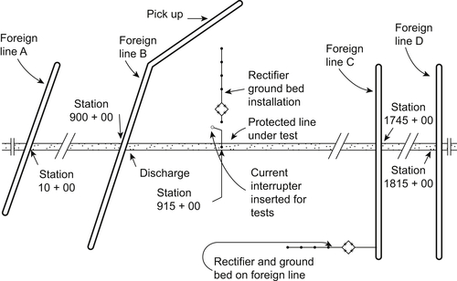
To perform the test, batteries will be sufficient as a source of power supply. A current interrupter automatically switches the circuit on and off (usually 30s on and 15s off). The interrupter also assures the inspector when at remote locations that the battery installation is operating properly and draining current from the pipeline as long as his potential and line current measurement continue to change in accordance with the established on–off cycle.
Test data may be taken for a section of 8km. Testing can be continued section by section in each direction from the power source until changes in the observed currents and potentials (as the current interrupter switches on and off) are insignificant. The length of the section that can be maintained at −0.85V or better will be established at the same time.
On coated pipeline systems provided with test points for potential and line current measurement, a survey will proceed rapidly. The survey can be carried out by a single inspector. For maximum accuracy, however, two engineers in radio communication can observe data simultaneously at each end of each section tested. This becomes essential if the pipeline under testing is affected by variable stray current.
Figure 6.9Coating resistance and CP current requirement tests.
To obtain data for the calculation of coating resistance, readings are taken for pipeline at each end of each test section as follows:
Potential readings to remote CSE with interrupter ON and OFF.
6.6.2. Pipeline Current with Interrupter On and Off
From these readings, the change in pipe potential (ΔV) with the change in line current (I) at each end of the section can be determined. The difference in the two ΔΔI values will be the test battery current collected by the line section when the current interrupter is switched on. The average of the two V values will be the average change in the pipeline potential within the test section caused by the battery current collected, namely, Δ.
The average V in millivolts divided by the current collected in milliamperes will give the resistance to the earth, in ohms, of the pipeline section tested. If one knows the length and the diameter of a pipe in the section tested, one can calculate its total surface area in square meters to be Δ.
Multiplying the pipe section to the earth resistance by the area in square meters will result in a value of ohms per average square meter. This is the effective coating resistance for the section tested.
Some inspectors express coating conditions in terms of coating conductivity in mhos or microhms. This is simply a matter of conversion. The reciprocal of the resistance per average square meter is the conductivity in mhos. The reciprocal times 106 is the conductivity in micromhos. A sufficient number of readings should be taken to ensure acceptable precision.
The following is an example of how this test method can be implemented:
• Test section
The Test Section is a 5000-m-diameter coated line that lies between Test Point 1 and Test Point 2. The wall thickness of the pipe is 9.52mm (0.375in).
Test data taken at test Point No. 1 are as follows:
Pipe/soil potentials (Reference CSE) are as follows:
−1.75V ON,
−0.89V OFF,
ΔV=−0.86V.
Potentials drops across test section are as follows:
+0.98mV ON,
+0.04mV OFF.
Span calibration is 2.30 Amperes per millivolt.
Pipeline current is as follows:
+2.25A ON,
+0.09A OFF,
ΔI=+2.16A.
Test data taken at test Point No. 2
Pipe/soil potentials (Reference CSE) are as follows:
−1.70V ON,
−0.88V OFF,
ΔV=−0.82V.
Potentials drops across the test section are as follows:
+0.84mV ON,
+0.02mV OFF.
Span calibration is 2.41A per mV.
B.6.3.2.4 Pipeline current
+2.03A ON,
+0.05A OFF (Negative current indicates current flow in the opposite direction),
ΔI=+2.08A.
Calculation of coating resistance
Average ΔV=−0.86+(−0.82)2=−0.84V.
Current collected is 2.16−2.08=0.08A.
Pipe-to-earth resistance=0.84V/0.08A=10.5 ohms
Surface area of the test section 4785m2.
Effective coating resistance 10.5×4785=50,242 ohms per average square meter.
Coating conductance is 10ˆ6/50,242=19.9 microhms per average square meter.
6.7. Test Method and Calculation for “Attenuation Constant”
Coating effectiveness of the pipeline may be evaluated using the attenuation method, which involves a limited number of field measurements.
The measurements lead to a figure that is termed “Attenuation Constant” per kilometer. From this figure, the spread of the protective current can be evaluated, and the approximate distance between drain points can be estimated.
When the original design fails to provide complete CP due to a sharp drop in the pipe/soil potential along the pipeline, the estimated distance would tell the designer where to put the rectifiers for supplementary protection. “Attenuation Constant” is derived from the attenuation equation. The equations describe the interrelation of factors affecting the degree of protection achieved at any specific location on a cathodically protected pipeline. The factors are as follows:
• Total current drain.
• Radial resistance of the path from the pipe surface to the remote earth. This factor includes both the resistance of the path through the coating on the pipe and the resistance through the soil.
• Diameter and the wall thickness of the pipe.
• Distance of the location from the drain point.
The basic formulas for attenuation are as follows:
dVx=dVoe−ax,
(6.12)
where dVx is the change in potential as distance×kilometers from the drain point in millivolts; dVo is the change in potential at the drain point with the cell directly over the pipe in millivolts; e is a constant 2.72 (base of natural logarithms); a is the attenuation constant in per kilometers; and x is the distance from the drain point in kilometers.
LndVx=LndVo+Lne−ax,
(6.13)
LndVx=LndVo−ax,
(6.14)
a=LndVo−LndVxX.
(6.15)
Equation (6.5) is the basis for constructing the attenuation graph for each value of attenuation constant. In addition to the above, it can also be shown that the following relationships apply:
a=RSRL,
(6.16)
where RS is the longitudinal resistance in the pipe wall (ohms per kilometer); RL is the leakage resistance or radial resistance from the pipe surface to the remote earth (ohms-kilometer).
RS=ρLA,
(6.17)
where ρ is the resistivity of the steel pipe usually estimated at 18 microhm-centimeterm unless actual resistivity is known; L is the unit pipe length, in this case 1km or 1×105cm; A is the cross-sectional area of the pipe in square centimeters.
RL=ρ2nLLnDr,
(6.18)
where ρ is the average resistivity of the soil around the pipe to remote earth in ohms centimeters; D is the distance from the pipe surface to effectively “remote” earth; r is the pipe radius in the same units as for D.
The following relationships are also applicable:
a=RSRK,
(6.19)
where RS is as shown in Eqn (6.17); and RK is the characteristic resistance of the entire line looking in one direction only from the drain point.
For a line uniform in both directions from the drain point,
PK=2RG,
(6.20)
where RG is the resistance of the entire line looking in both directions from the drain point.
RG=dV′odI,
(6.21)
Here,dV′o is the change in the potential at the drain point related to a remote cell; dI is the current–drain change that causes dV′o.
From this,
RK=2dV′odI,
(6.22)
a=RSdI2dV′o.
(6.23)
For a line on which there are rectifiers spaced at a distance 2AL kilometers apart, the relationship is as follows:
dVm=dVocoshal,
(6.24)
where dVm is the change in potential at the midpoint between rectifiers.
Practically, the same value for dVm is obtained if the following two values are added:
dVAL=dVAoe−aAL,
(6.25)
dVBL=dVBoe−aBL,
(6.26)
where values (dVAL), (dVAo), and (aA) all relate to rectifier (A).
dVm=dVAL+dVBL.
(6.27)
6.7.1. Significance of Attenuation Constant
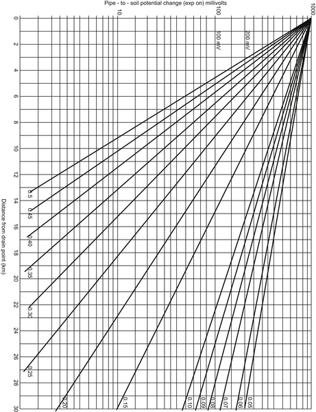
To put the various levels of attenuation constant in perspective, a graph showing the effective spread of protection for various values of attenuation constants (from 0.05 to 0.5 per kilometer) has been prepared (Fig. 6.10).
6.7.1.1. Method of Calculation
It is assumed that the potential change at the drain point is to be 1000mV from the static pipe/soil potential.
Thus, if the static pipe/soil potential is about 500mV, the maximum pipe/soil potential would be 1500mV (all potential values are with reference to the CSE).
To construct the graph, the value of the potential change was calculated for the 10-km distance for each value of attenuation constant, and the value so calculated was plotted on the 10km line.
A straight line was then drawn from Δ=1000 at km zero through the point plotted at km 10 for the particular value of “a.” V.
For example,
If V=1000 Δ,
X=10km,
a=0.50 per km.
LnΔVx=LnΔVo−ax=6.90−(0.5×10)=1.90,
(6.28)
ΔVx=6.7.
Figure 6.10Graph spread of protection relating to the attenuation constant.
6.7.2. Example Use of Graph Relating to Attenuation Constant
If the static potential is assumed to be −500mV to the CSE and the desired minimum potential is −900mV to copper sulfate (allowing a 50-mV safety factor), then the minimum potential change due to each rectifier at the midpoint (between rectifiers) would have to be as follows:
900−5002=200mV.
(6.29)
From the graph, it will be seen that the distance from the drain point at which this potential change (200mV) is just achieved is a function of the attenuation value.
For instance, if the attenuation constant is 0.45 per km, the distance at which the potential change attainable is 200MV is 3.6km. To achieve protection to the 900-mV minimum level with this value of attenuation constant, it would be necessary to space the rectifiers 2×3.6 or 7.2km apart. To put the various levels of attenuation constant in perspective, a rating table has been prepared. This table can be used to describe the relative effectiveness of any coating, as installed, in terms of attenuation constant per kilometer of the line concerned. Based on the attenuation constant value, the approximate distance between drain points can be estimated, and the location for installation of a new rectifier to supplement ineffective CP system may be decided.
6.8. Coating Inspection by the Pearson Method
The Pearson survey is an above-ground survey technique used to locate coating defects in buried pipelines and is named after J.M. Pearson who developed the technique. The survey compares the potential gradients along the pipeline measured between two movable electrical ground contacts. The potential gradients result from an injected alternating current (AC) signal leaking to the ground at coating defects or metallic objects within the pipeline trench.
6.8.1. Equipment
The equipment required for the survey comprises the following:
• Transmitter to provide an AC signal of approximately 1000Hz for conventional pipeline coatings, for example, enamel, tape, extruded coating, and a reduced frequency of 175Hz for thin film coating, for example, fusion-bonded powder epoxy. The transmitter is powered from internal batteries or for long surveys from an external high-capacity battery.
• Receiver, hand-held, self-contained, battery operated with pick-up sensitivity controls, audible warning, earphone output, and, in some cases, recording capability. The receiver is tuned to the transmitter frequency.
• Earth contact set of boot cleats, studded boots, or modified aluminum ski poles.
• Connecting cable harness between earth contacts and receiver.
• Earth spike and connecting cables for the transmitter.
The above equipment is normally all contained in a portable box for easy transportation. The total weight is approximately 25kg.
Optional equipment available from some suppliers enables the instrument to be used as a general-purpose pipe/cable locator and comprises the following:
• Signal level meter on receiver.
• Pipe location antenna.
• Pipe depth indication.
• Signal recorder and playback chart recorder or interface to a portable computer.
6.8.2. Procedure
The equipment is set up as shown diagrammatically in Fig. 6.11. The transmitter is electrically connected with one lead to the pipeline, usually by connecting to a CP test lead or an accessible part of the pipeline, and the other lead to a good remote earth and then energized.
Using the receiver in the pipe locating mode, or a separate pipe locator, one can locate and identify the section of pipe to be tested so as to enable the survey operators to follow the route of the pipe exactly above the pipe. For record purposes, it may be useful to insert pegs at measured intervals.
The survey may be carried out with an impressed current CP system energized. However, any sacrificial anodes, bonds to other structures, or similar are best disconnected before commencing the survey to ensure that they do not mask defect areas or drastically reduce the length that may be surveyed from one injection point. With the line located, the receiver is then connected via the cable harness to the earth contacts worn or held by the two operators such that at all times, earth contact is made by each operator. The connecting cable provides for a separation of 6–8m between the operators.
Surveying should commence at a sufficient distance from the transmitter and earth spike to minimize interference from the transmitter and/or return current flow in the earth.
The two operators walk over the top of the pipeline to locate coating defects. When the front contact approaches a defect, an increased signal level is indicated in the earphones by an increase in volume or by a higher reading on the receiver signal level meter. As the front contact passes the defect, the signal fades and then peaks again as the rear contact passes over the defect.
The defect is logged on the record sheet at a measured distance from a reference point (by triangulation if possible) and/or may be indicated with a marker or nontoxic paint. The signal is recorded automatically for later interpretation if the receiver is fitted with recording equipment. Where the signal is not easily interpreted or where there may be more than one defect within the span of the operators, this may be clarified by surveying at right angles to the pipeline, that is, one operator walks over the pipeline and the second walks parallely to the pipeline at 6–8m from the pipeline. In this mode, each defect is indicated as the operator over the pipeline traverses the fault. This is utilized when using recording equipment.
Figure 6.11Typical signal level on passing a coating. (a) Low signal (b) High signal (c) Low signal (d) High signal (e) Low signal.
The above procedures are general, and in all cases, the equipment manufacturer's instructions are to be followed.
6.8.3. Data Obtained
The information obtained from a Pearson survey is the change of signal intensity at probable defect locations.
For instruments without a signal level meter, only the location and the operator's aural interpretation of the signal strength can be recorded. Where a signal level meter is fitted, further data concerning the rate of increase and decrease and the maximum signal level may be recorded, together with intensity variations around the defect location, which can assist in analyzing the magnitude and disposition of the defect. This is done automatically when the receiver is of the recording type.
6.8.4. Presentation of Data
Defect indications are either by audible tone or by the signal meter level. The accuracy of recording signal level changes either manually or automatically, and the locations where they occur are very important to enable further investigations to be carried out.
Locations of probable defects can be measured to fixed points so that they may be returned to at a later date.
In addition to recording the probable defect locations, valuable information may be gained by recording various observations of the signal levels on the meter, which will assist in the evaluation of the probable defect. For example, if the signal level rises to a peak rapidly and then falls away, or if it rises steadily and remains high for a distance before decaying, these characteristics may be recorded. This is done automatically if the receiver is of the recording type.
The survey record sheet may provide space to adequately note all pipeline features, reference points, other services crossing, signal intensity levels, and characteristics, etc. to enable the results of the survey to be analyzed and determine areas where further investigations or remedial measures are required.
Where repeat surveys are carried out, these records can be compared and may show further deterioration of the condition of the coating.
6.9. Coating Inspection by the C-Scan System
This system introduces the latest technique of above-ground coating inspection. The system locates coating defects on buried pipelines and provides an assessment of external coating quality. In addition to the coating condition, the system can also be used to locate contact or connection points between buried services, which can be of great importance in the proper functioning of pipeline CP. The system is based on current attenuation survey. The current attenuation is the only technique that gives a value (attenuation) that is a direct indication of the pipeline coating.
Excavations confirmed almost all defect locations detected by C-Scan. The C-Scan located the defects found by the Pearson survey and also located defects that the Pearson survey did not find. At the end of a survey (or whenever required), the detector unit may be plugged into any computer or printer, and the survey report can be printed out in full. Alternatively, the data can be displayed on a computer monitor or stored on disk or tape for further analysis.
The coating condition of a pipeline can be monitored over its working life. This is done by repeating the general survey at intervals of three to five years. The results of the repeat surveys are compared with those from the first survey to monitor any deterioration of the coating with age (aging effect on coating condition).
6.9.1. C-Scan System Features
Operation of the C-Scan detector is largely automatic. When required, prompt messages, instruction messages, and warnings are displayed to the operator to guide him through the survey sequence.
The operating frequency of the system has been selected to minimize interference from commonly occurring sources. The filtering system and the directional nature of the detector antenna help to eliminate almost all suspicious signals. The C-Scan system includes the following items:
• Signal generator with built-in charger.
• Generator/pipe connector lead.
• Generator/earth connector lead provided with extension. Set of earth spikes, complete with connector leads.
• Detector unit containing power pack, antenna, and computer.
• Spare power pack for the detector unit.
• Charger for the detector power packs.
6.9.2. Performing Survey by C-Scan
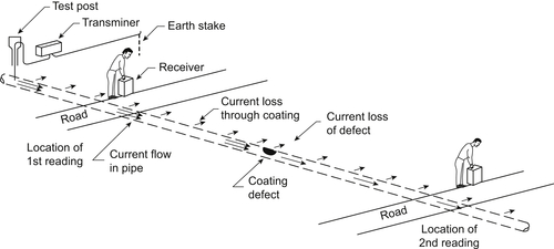
The C-Scan system uses a generator to apply an AC signal to the pipe, and this is done by connecting one of the generator output leads to the pipeline at a CP test point, valve, or access point; the other lead of the generator is attached to a remote earth.
A constant AC signal (set by the operator) is applied to the pipeline. The applied AC signal will flow along the pipeline in both directions, decreasing in magnitude as the signal leaks to the earth through the coating. At coating defects, where the pipeline is in direct contact with the soil, the signal leakage to earth is greater.
A detector is used to measure the strength of the AC signal on the pipe. The operator starts making measurement. The first measurement is made at least 100m from the point of injection, usually at a fence or other identifiable feature. The detector will automatically take 1000 readings of the magnetic field and will compute and display to the operator the depth to the center line of the pipeline and the signal level (strength of the remaining signal current). If required, the detector unit will also record (store) these data and give them a (marker) number for subsequent reference.
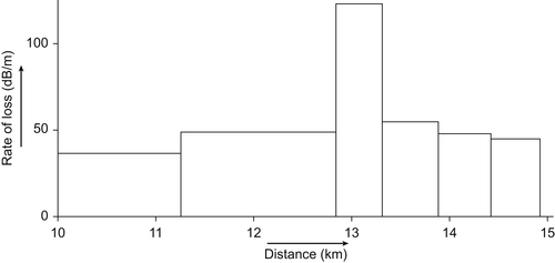
This procedure is then repeated at the next survey point, usually the next road crossing or the next cathodic test point. The attenuation is calculated from these values and gives a direct indication of the coating condition in that section.
An initial survey, called the general survey, may be carried out on a pipeline by taking measurements at road crossings and points of easy access with intervals of approximately 1km. This will identify the sections of the pipeline between measurement points where coating defects exist. The defect location may be defined by progressively halving the distance in the suspect section until it has been reduced to a practical length where a detailed close interval current loss survey can be carried out.
6.9.3. Advantages of the System
The main advantages of this system are as follows:
• Rapid assessment of the system.
• Accurate defect location and depth determination.
• Repeating the survey at regular intervals to monitor coating condition during the working life of the pipeline.
• Survey can be carried out in plant areas where the pipe is covered by concrete or tarmac.
• No need to walk the entire length of the pipeline and areas of difficult access, such as rice fields, etc.
• Survey includes road, rail, and river crossings.
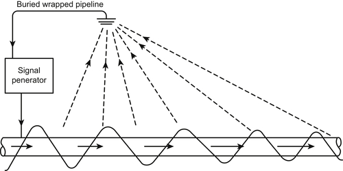
6.9.4. Theoretical Background
An electrical current applied to a well-wrapped buried metal pipeline will decrease gradually with increasing distance from the current injection point, as the current escapes to the earth through the coating.
If the coating has a uniform thickness and separates the pipe from the surrounding soil at all points, the strength of the signal current on the pipe will decline logarithmically, and the rate of decline will be dependent primarily on the effective resistance of the coating in use (resistance per average square meter of coating), and the area of coating in contact with the soil per unit length of pipe (i.e., for a given coating, the decline is proportional to the circumference of the pipe).
It should be borne in mind that because of the relative magnitude of the resistance involved, local changes in soil resistivity can usually be ignored.
If there is a low resistance electrical path from the pipe direct to the soil at any point, there will be a substantial local increase in the rate of loss of signal current. Such a low resistance path could arise from the following:
• Improper applied coating.
• Mechanical damage to the coating before, during, and after application.
• Decay of the coating due to soil stress or bacterial effects.
• Disbonding of the coating from the pipe (provided that ground water has penetrated into the gap to create an electrical path to the earth).
• A leak in the pipe itself causing the coating to fail at the leak point.
Because the resistance of such an electrical path to the earth is likely to be several orders of magnitude less than the resistance of the undamaged coating, the resultant loss of current, even from a single small fault of a few square millimeters, can usually be detected by a significant increase in the apparent rate of current decline over quite a long length of pipe.
In practice, the existence of one or two small faults on a section of pipeline several hundred meters in length can usually be tolerated because CP system is expected to prevent corrosion resulting from these faults. In this case, it may not be necessary to locate the specific faults immediately, but the rate of the logarithmic decline of the current between two specific points can be logged for future reference so that any deterioration of the condition of the pipeline coating can be monitored.
The logarithmic rate of decline of the current (which is known as attenuation level) is measured in terms of millibels (1/100 of decibel) per meter. This rate of decline of the current is effectively independent of the applied current so that it is virtually an absolute indication of the average condition of the coating between two given points at the date on which the survey is made.
If the attenuation level over a given section of pipeline is particularly high, serious faults (or a large number of small faults) in the protective coating are indicated. Intermediate readings of attenuation levels can be taken to identify the worst sections. The survey can be made extensively over the suspect section at close intervals (3–5m), and readings of the actual current levels in this section can be taken, recorded, and plotted. By so doing and noting the place where the rate of current decline is the steepest, the precise location of faults (generally to an accuracy of 1–2m) can be determined. This locates the defect to the extent that excavation for visual check and repair is justified.
6.9.5. Operation Principle
As mentioned earlier, this system of coating evaluation is based on current attenuation level. The main operating components of the system are “The Signal Generator” and “The Detector Unit.”
The Signal Generator is attached to the pipeline and also to an appropriate earth point, and produces a constant AC signal that passes along the pipe.
The detector unit measures the electromagnetic field radiating from the pipeline and uses this to:
1. Locate the pipeline.
2. Determine the depth of the pipe.
3. Determine the residual strength of the signal current at the observation point.
The above data can be stored in the memory of the detector unit's computer and are used to compute and store current attenuation rates between any two given observation points.
The complete record of the survey (with time and data) may be printed out at the end of the survey to provide a permanent record.
6.9.5.1. Signal Generator
The C-Scan signal generator contains the following:
Power supply consisting of six 12-V batteries. Capacity of each battery is 5A/hr.
A built-in charger suitable for a mains input of 110 or 240-V single phase with a frequency of 50 or 60Hz, respectively.
The inverter–frequency changer that inverts the output of the signal generator to a sine wave signal at a frequency of 937.5Hz, with a nominal maximum voltage of 60V.
The maximum current obtainable is approximately 1A. The Root Mean Square value of the current being produced is displayed on the digital ammeter of the instrument. The value is expressed in milliamperes.
The actual level of current produced is set by the surveyor using the instrument's controls. Once set, this current level will be maintained at a constant level (despite any transient changes in soil resistivity), until the batteries are exhausted. In tests, the unit when fully charged has maintained a constant output of 750mA for up to 16h of continuous operation.
6.9.5.2. Detector Unit
The detector unit consists of two vertical tubes joined by two smaller crosstubes, the upper one of which serves as a carrying handle. The taller vertical tube contains parts as given hereunder:
• The antenna system.
• The keyboard and liquid crystal display (LCD) that are mounted on the top of the tube.
The other vertical tube contains the computer, the power supply, and the printer lead. The antenna consists of five large-diameter air cored coils. Two of these are at the bottom of the tube with their axes horizontal and at right angles to each other (c and d). Another identical pair (a and b) is at the top of the tube approximately 80cm above the first pair, and a fifth coil with its axis vertical.
6.9.5.3. Principle of Operation
In operation, the computer calculates the vector sum of the field strength measured by the two pairs of coils (ab and cd) and indicates to the operator that it has acquired the signal radiating from the buried pipe. The LCD gives an indication of the field strength and guides the operator toward the pipe. A comparison of the field strengths at the top and bottom of the antenna, with the strength of the field measured by the vertical axis (e) coil, is used to inform the operator when he is close to the pipeline.
When the field measured by the (e) coil falls below a threshold value, the instrument informs the operator to stop because is overhead. Once the instrument is stationary in the overhead position for a few seconds, it will automatically collect a sample of 200 readings of the field strength values at the top and bottom of the antenna over a period of approximately 4s. Provided the standard deviation of the sample is below a threshold value, the computer will calculate the depth of the pipe (below the center of the bottom coil pair) and the strength of the residual signal current on the pipe.
The depth (in meters) and current value (in milliamperes) are shown on the LCD for a few seconds, and if the operator takes no action, the instrument will repeat the sample and calculation routine.
Using the keyboard and, following the prompts appear on the display, the operator can store the display data (which is mathematically given a reference number), and request the computer to calculate the logarithmic attenuation of the signal from any previous location stored in its memory. This information is displayed on the LCD and may also be stored if required. The computer can store up to 100 complete sets of data (location reference number, depth of pipe, strength of signal current, distance from a previous location reference, and logarithmic attenuation of the signal), in millibels per meter, between the two points. At the beginning of each survey, the computer will also automatically note the time and data using its internal clock. This information will also appear on the subsequent printout. Current readings obtained in the course of a close interval survey to locate specific faults are not stored for printout, as they are unlikely to be relevant to subsequent surveys. These readings are generally noted down for plotting purposes by the operator during the course of the operation.
At the end of a survey (or whenever required), the detector unit may be plugged into a standard computer printer, and the survey report may be printed out. Alternatively, the data may be displayed on a computer monitor or stored on disk or tape for further analysis.
The detector unit is powered by a nickel–cadmium rechargeable power pack providing enough power for continuous running for over 20h.
In addition, there is a separate built-in lithium power source to maintain the data stored in the memory and the operation of the clock, when the power pack has been unplugged. This power source has an estimated life of 10 years.
The C-Scan system is not immune to electromagnetic interference, but it incorporates a number of features that are designed to keep such interference to a minimum. The feature include the following:
1. The generation of a pure sine wave so that no complex harmonics are produced.
2. The use of a carefully selected frequency with virtually no harmonics in common with other frequencies in general use.
3. The collection of 200 signal “samples” over a period of approximately 4s to eliminate transient interference.
The instruments are not affected by the presence of mains AC current, nor does any residual ripple of CP rectifier affects the operation of the system.
6.10. Coating Evaluation by Electromagnetic Current Attenuation Survey
The electromagnetic current attenuation survey is an above-ground survey technique used to locate coating defects on buried pipelines and to provide a comparative assessment of coating quality.
An AC signal is applied between the coated pipe and remote earth. When the signal current flows along a straight conductor (pipeline), it creates a magnetic field, cylindrical in shape, around the pipeline. The shape of this field is not affected by the presence of pipeline coating, by different types of soil, or nonreinforced concrete, tarmac, etc. It is possible by electromagnetic induction to detect and measure the intensity of this signal with an antenna.
Figure 6.12Current attenuation.
The applied AC signal will flow along the pipeline in both directions, decreasing in magnitude as the signal leaks to the earth through the capacitive and resistive effects of the coating. At coating defects, where the pipeline is in direct contact with the soil, the signal leakage to the earth will be more significant (Fig. 6.12).
Thus, signal losses over a section of the pipeline are due to the following:
• Dielectric and resistive losses due to the nature and quality of the coating.
• Capacitive losses of the AC signal to earth.
• Discrete points of coating damage resulting in steel/soil contact.
• Metallic contact with other buried conductors.
Where the current is observed to attenuate at a constant rate over a long section of the line, these losses are due to the intrinsic characteristics of the pipeline coating rather than resulting from evenly spaced holidays of a similar area. Where a metal-to-soil contact exists, the signal loss greatly increases at this point, clearly indicating the presence of a coating defect.
6.10.1. Equipment
The equipment required for the survey comprises the following:
• Transmitter to provide an AC signal of approximately 1000Hz. Thin-film coatings may require a reduced frequency in the order of 200Hz. The transmitter is powered from internal batteries. Longer surveys may require the use of an external high-capacity battery.
• Receiver, hand held with integral antenna for monitoring and indicating the location of pipeline, depth of pipeline, and signal strength of the electromagnetic field.
• Earth spike and connecting cables for the transmitter.
The above equipment is normally contained in a plastic or aluminum box. Its total weight is between 15 and 30kg, dependent on the manufacturer's guidelines.
Some equipment is fitted with a microprocessor control that enables current flow and attenuation rates to be computed and data to be stored and printed out on completion of the survey. Optional equipment available may enable the instrument to be used for general-purpose pipe/cable locating, Pearson survey, etc.
6.10.2. Procedure
The equipment is set up as shown in Fig. 6.13. The transmitter is electrically connected with one lead to the pipeline, usually by connecting to a CP test lead or any accessible part of the pipeline, and the other lead is connected to a good remote earth. The transmitter is energized and set to the appropriate output.
The survey may be carried out with an impressed CP system energized. However, any sacrificial anodes, bonds to other structures, or similar are best disconnected before commencing the survey to ensure that they do not mask defect areas or cause excessive signal loss, thereby reducing the length that may be surveyed from one transmitter location.
The first measurement is made at a sufficient distance from the transmitter and earth spike to minimize interference from the transmitter and/or return current flow in the earth. The receiver “location” mode is used to accurately position it directly above the pipeline.
The depth to the center line of the pipeline and the signal level, corrected for depth, is measured and recorded.
This procedure is then repeated at the next measurement point. Subtraction of the two values gives the signal loss between the two measuring points. To calculate the attenuation rate, the signal loss is divided by the distance between the two measuring points. This may be computed manually or by an in-built microprocessor.
Figure 6.13Principle of electromagnetic current attenuation survey.
As the survey proceeds, measurements are taken at intervals until the intensity of the signal is insufficient to be monitored accurately. At this point, the transmitter is moved, and the above procedures are repeated for the next section of the pipeline.
The length of the pipeline surveyed from any one transmitter location may vary from <200m to in excess of 20km depending upon the quality of the pipe coating, the size of the pipeline, the resistivity of the soil, etc.
A survey cannot be conducted over the last 2–3km of a well-coated pipe or 0.5km where high losses are present working toward an electrical isolating device. Either the transmitter should be located at the isolating device or the device should be temporarily bonded across.
An initial survey may be carried out on a pipeline by taking measurements at road crossings and points of easy access with intervals of approximately 1km. This will identify sections of pipeline between measurement points where coatings defects exist. The defect location may be defined by progressively halving the distance in the suspect section until it has been reduced to a practical length where detailed measurements would then be applied.
Measurements are to be avoided at locations where pipe bends or other metallic services are present as there will be a distortion of the magnetic field giving erroneous readings.
The above procedures are general, and in all cases, the equipment manufacturer's instructions are to be followed.
6.10.3. Data Obtained
The data recorded from an electromagnetic current attenuation survey would be as follows:
• Location reference.
• Chainage.
• Distance between measurements.
• Depth.
• From these data, the following may be calculated:
• Signal level attenuation.
• Signal level attenuation rate.
6.10.4. Presentation of Data
The results of the survey may be presented in one of the following formats:
1. Tabular.
2. Graphical—plot of signal level against distance (Fig. 6.14).
3. Histogram—plot of section attenuation or attenuation rate against distance (Figs 6.15 and 6.16).
Figure 6.14Plot of signal level vs distance.
Figure 6.15Plot of signal loss vs distance.
6.10.5. Criteria and Interpretation
The criteria for determining the coating quality are not precise and differ from one pipeline to another.
The attenuation rate is primarily dependent on the overall quality of the coating and the coating area per unit length of pipeline, that is, it is a function of quality and circumference. “Quality” is related to a combination of the following: type of coating, general age and condition, and the presence or absence of discrete faults due to mechanical damage or other factors. Attenuation rates are not affected by changes in wall thickness and are only marginally affected by changes in soil resistivity except in extreme situations such as in deserts or where there is very poor or nonexistent coating over long lengths of pipe.
Figure 6.16Plot of rate of loss vs distance.
From the data, the average attenuation rate of the pipeline can be determined. Any significant change of gradient on the graph or increase in the section attenuation rate on the histogram may be treated as a suspected defect.
Where intervals of measurement are irregular or are very small, the histogram plot of attenuation rate against distance may be misleading, and a plot of attenuation against distance may be preferred.
A high signal loss may not be present at a substantial coating defect in high-resistivity soil. Because of high soil resistivity, the loss of current will be restricted. However, the corrosion risk at such an undetected defect will be reduced since the corrosion current would also be restricted by the high soil resistivity. Signal level is corrected for depth.
6.11. Close Interval Pipe-to-Soil Potential Survey
The close interval pipe-to-soil potential survey is a survey technique to provide a detailed profile of the potential difference between the steel and the soil. This profile can be used to determine detailed information on the performance of the CP system, the coating system, interaction effects, etc.
The performance of CP systems has normally been monitored on a sample basic, that is, pipe-to-soil potential measurements taken at test stations installed at intervals of approximately 1km along the route of the pipeline.
Based on this information, a judgment is made of the performance of the CP system and also, by inference, the performance of the pipe coating system.
If a defect of any kind occurs on a pipeline at a location remote from a test station, it is probable that this will remain undetected. It has therefore become apparent that a much greater sample of pipe-to-soil potential measurements, representative of the pipeline as a whole, needs to be collected to ensure that the corrosion prevention systems are performing satisfactorily.
To achieve this, it is necessary to place the reference electrode at a much greater number of locations than the number of test stations. Close interval potentials are generally measured at between 1- and 5-m spacing to provide a “continuous” pipe-to-soil potential profile of the structure.
Equally essential is the need to reference, record, and store the data collected and to present the larger number of measurements in tabular and/or graphical form.
The methods and measurements utilized are based on methods used in everyday routine monitoring procedures. The advent of portable microprocessor-based measuring equipment and computer-assisted data handling, together with accurate, synchronized high-speed current interruption devices, have allowed these surveys to provide practical data collection methods that are of value when assessing the performance of the corrosion-prevention systems applied to buried pipelines.
The potentials may be recorded with the CP system permanently energized as in routine “on” surveys. However, these measurements will include the IR drop error caused by the flow of CP currents in the soil.
To eliminate this error, cyclic timers are fitted to the transformer rectifiers or to other DC power sources to interrupt the CP current. Potential measurements are then recorded with the CP switched on and immediately after switching off (IR drop error-free or instantaneous off measurement) over the entire length of the pipeline. It is of utmost importance to ensure that all power sources that can influence the pipe-to-soil potential at the point being measured are switched in unison by the use of synchronized timers. Surveys measuring the “Instantaneous Off” potentials are commonly referred to as “polarized” potential surveys. This method is not practical for use with distributed sacrificial anode systems.
In areas of stray current interaction where the pipe-to-soil potentials are not stable, stationary data collectors may also be used.
The foregoing covers the general requirements for a close interval potential survey. However, when planning to carry out a survey, the following practical considerations may be kept in mind:
• The need for mobile operation to traverse the pipeline length and obtain data at a reasonable speed.
• The requirements for current interruption to switch the CP current sources at high speeds, at a ratio that will not depolarize the CP levels and with a minimum of synchronization error.
The need for polarized potentials to be collected at such intervals to provide an accurate profile of IR drop error-free measurements.
• The need for switching cycle and distance between readings to be so arranged that the measurement equipment records accurately with respect to instrument stabilization and synchronization errors.
• The method by which equipment operates and data are recorded, that is, manual, semiautomatic and automatic.
6.11.1. Measurement Intervals
The measurement intervals between pipe-to-soil potentials may be determined by the pipe diameter and the depth of cover over the pipeline.
For pipeline diameters of ≤600mm, a minimum spacing of 1m is appropriate, although specific circumstances may necessitate closer intervals in order to determine particular characteristics.
For pipeline diameters in excess of 600mm, a 1-m spacing is appropriate, but this may be increased. The measurement interval should not, however, be >1.5 times the normal pipeline depth of cover or 5m whichever is the smallest.
In practice, polarized measurements are commonly taken at
• Every meter,
• Every 5m,
• Ratio of 4 “on” readings and 1 “off” reading, each reading being taken at meter intervals.
6.11.2. Switching Frequency
The switching frequency of the CP and associated equipment required to enable pipe-to-soil potential measurements to be made, may be determined by the following factors:
• The degree of synchronization that can be achieved between the timers.
• The measurement response time of the data collector.
• The measurement interval of pipe-to-soil potentials in automatic time-dependent surveys.
An important consideration in the selection of time cycles is the provision of long-term switching (during the survey period) without any degradation of the polarized potential level due to the “off” period. Depolarization will cause inaccurate and unreliable potentials to be measured. For this reason, a minimum on/off ratio of 4:1 is common practice. This assumes that the quality of the measurement circuit will provide for a stabilized accurate measurement during the “off” period (response time) and that the synchronization error between switching devices does not conflict with the measurement period.
Switching of the CP equipment may be by devices interrupting either the AC or DC side of the transformer rectifier or other power sources and may be either built in or fitted for the duration of the survey. The current interrupts must have the facility to switch at high speeds, cause minimum transient switching surges, have a selection of commonly used time cycles, and have <100-ms synchronization error between devices and maintain this for a minimum of one working day. An image retaining oscilloscope or high-speed recorder may be used to verify that no significant depolarization occurs with the time cycle selected and that timers are fully synchronized.
If switching is carried out on the AC supply, the polarized potential measurements may adversely be affected by the unbroken connection of the pipeline to the ground bed via the DC power source, allowing some currents still to flow.
6.11.3. Distance Measurement
The survey needs to have some means of distance measurement with respect to the mobile potential data collector. Systems are available to accurately record the distance from a fixed point that can be related to pipeline chainage. Basic systems operate with annotating pipeline chainage at the start and finish of each survey section.
For more details, a pedometer or chainer can be used, and the distance is keyed into the data collector. With fully automatic systems, a wire measurer is often used, which can give an accuracy to within a few meters per kilometer.
All systems need to allow for chainage to be entered, together with any physical features found along the route of the pipeline so that defects indicated on the plots may be physically located.
6.11.4. Stationary Measurements
In areas where stray interaction currents or variable potentials may be present during the mobile survey, stationary data collectors may be employed at fixed locations on the pipeline as close as possible to the anticipated point of maximum interaction. Stationary measurements may be obtained at one or more of the following locations:
• Start and finish of surveyed section.
• Anticipated locations of maximum interaction effect.
• Locations close to the mobile unit.
The data collected from the “mobile” unit can then be compared with the data from the “stationary” unit. If fluctuations of potential on the “mobile” plot coincide with similar fluctuations on the “stationary” plot, this is indicative of interaction or stray currents and not necessarily due to inadequacies of the corrosion protection system. The data collected are therefore to be accurately time related in order to make this comparison.
6.11.5. Equipment
The equipment required for the survey varies from very simple manual equipment to complex microprocessor/computer equipment.
In general, the equipment comprises the following:
• Synchronized timers for switching the transformer rectifiers or other DC power supplies (not required for “on” surveys).
• Data collector with input impedance in excess of 10 Megaohms with an adequate level of AC rejection which may be
• Manual—voltmeter/multimeter.
• Semiautomatic—recording voltmeter.
• Microprocessor data collector with manual entry.
• Automatic—microprocessor data collector with fully automatic recording of data.
• Cu/CuSO4 reference electrode(s) fitted to pole(s).
• Insulated fine wire that may be reusable or disposable, wound on reels.
• Distance measurer that may be
• Chainer.
• Pedometer.
• Wire measurer that automatically measures the length pulled off the fine wire reel and records the value in the data collector.
• Pipeline location equipment.
• Computer hardware and software for processing the data.
• Plotter for producing the profile plots.
6.11.6. Procedure
Before commencing the survey, the exact route of the pipeline is located and marked out so that the survey operator may follow the route of the pipeline exactly over the pipe. Alternatively, a pipe location operator may immediately precede the survey operator to minimize the working period over the pipeline route.
If polarized potentials are to be measured, timers are synchronized and installed in all transformer rectifiers or other CP power supplies, bonds, or other connections that may influence the potentials over the section of pipeline to be surveyed.
If the survey is subject to interaction or fluctuating potentials, stationary recording units would be installed.
With the equipment connected and the pipeline located, the survey operator, carrying the mobile data collector and Cu/CuSO4 reference electrode(s), traverses the pipeline paving out the fine wire and placing the reference electrode at the required interval over the pipeline and maintaining it in that position long enough for the data collector to measure and store the pipe-to-soil potentials. Alternatively, two reference electrode(s) may be fitted to poles such that one reference electrode is always in contact with the ground. Distance traversed and physical features, such as roads, hedges, and streams, are recorded to assist with locating specific areas after processing the data.
As each section between pipeline connection points is completed, the fine wire is either re-reeled for further use or recovered and properly disposed of, to prevent a hazard to livestock. Where the fine wire crosses roads, paths, or fields, with livestock present, the wire may be pegged down.
The data are usually transferred from the data recorder to a computer for producing data printouts and plots of the pipe-to-soil potential profiles.
The above procedures are general, and in all cases, the equipment manufacturer's instructions are to be followed.
6.11.7. Data Obtained
The data obtained from a close interval pipe-to-soil potential survey include the following items:
• Time.
• Date.
• Distance (pipeline chainage).
• Locations.
• Energized potential.
Polarized potential.
• Physical route features.
• CP power supply outputs.
• Bond currents.
6.11.8. Presentation of Data
The data collected during the survey are normally processed by a computer and presented in tabular and graphical form.
The raw data are normally processed immediately following the completion of each day's survey to verify the full functioning of the survey equipment and identify if any areas may require resurveying due to interaction, equipment malfunction, etc.
Plotted profiles are produced at a later date when all the data have been processed.
The data presentation is normally computer assisted. This allows for data to be organized in the correct chainage order regardless of survey direction and section order.
6.11.9. Criteria and Interpretation
The criteria used for closed interval pipe-to-soil potential surveys are the same as those used for routine potential surveys.
The close interval survey enables the potential profile for the whole length of the pipeline to be plotted. With the CP system switching “on” and “off,” and polarized potentials, free of IR drop error, measured, a profile of the true pipe-to-soil potential can be determined.
It is the measurement of the polarized potential that determines the effectiveness of the CP current in both qualitative and quantitative terms.
Any areas on the profile that fall outside the selected potential criteria are not being provided with adequate CP and could therefore be corroding. Interpretation of the pipe-to-soil potential profile may highlight the following:
• Coating defects.
• Underprotected sections of pipe.
• Interaction by stray currents.
• Overprotected sections of pipe.
6.12. An Example for Cathodic Field Interference Test Method
To illustrate the interference test method, assume that a CP system incorporating a rectifier as the power source has been applied to a section of coated pipeline and that there are several pipeline crossings in the section as shown in Fig. 6.17.
Figure 6.17An example for cathodic field interferences.
Assume that at each foreign line crossing a test point has been installed, as shown in detail in Fig. 6.18, with two color-coded leads brought to the test point terminal from each point.
With the current interrupter operating, each foreign line crossing is visited and the potential of each line is measured under both current “ON” and current “OFF” conditions. For these tests, the CSE is placed directly over the point of crossing. If there is any question as to the crossing location, use a pipe locator to determine where it is. Data taken at the several pipeline crossings of Fig. 6.18 may be recorded as shown in Table 6.2:
Figure 6.18Testing foreign pipeline crossings for stray current interference from CP installations.
Table 6.2
Survey Notes on Stray Current Investigation
Foreign Line Designation and Location
Potential vs Close Copper/Copper Sulfate Electrode
Own Pipeline, V
Foreign Pipeline, V
Name
Pipeline Station
With Current
With Current
On
Off
ΔV
On
Off
ΔV
A
10+00
−1.03
−0.98
−0.05
−1.02
−1.04
+0.02
B
900+00
−1.98
−1.02
−0.96
−0.32
−0.68
+0.36
C
1765+00
−0.68
−0.64
−0.04
−0.78
−0.78
0
D
1815+00
−1.10
−1.06
−0.04
−0.68
−0.68
0
Data entered have been selected to illustrate various types that may be encountered. In addition to the data shown for this illustration, field data sheets should include full information on the line protected; this includes data, current output of the interrupted rectifier, and other pertinent facts.
The following are some conclusions that can be reached from the data:
Crossing A
Pipeline under test is fully protected but can be expected to have a substantial coating holiday in the vicinity of the crossing. This is based on the fact that the potential of the foreign line (which is also cathodically protected) decreases when the interrupted rectifier switches from “OFF” to “ON.” This indicates that there is appreciable current flowing to the line under test, creating more negative soil locally around the foreign line.
The foreign line in this instance is cathodically protected as indicated by the fact that although its potential at the crossing is reduced by the operation of the rectifier on the line under test, the reduction is not sufficient to indicate any loss of protection. On the basis of the data shown, no corrective measures would be required at Crossing A.
Crossing B
Pipeline under test is fully protected. The foreign pipeline is not cathodically protected because its potential is well below 1.0V (with the rectifier “OFF” on the line under test). With the rectifier ON, the foreign line potential is shifted severely in a less negative direction, indicating the probability of severe corrosion damage to the foreign pipeline. Corrective measures will be required.
Crossing C
The line under test is receiving inadequate CP, apparently because of interference from the cathodically protected foreign line. If the potential of the line under test to a remote electrode with respect to both lines and this potential is found to be representative of normal protective potentials (above −1.0V), the poor potential at the crossing is shown to be a local condition probably caused by the foreign line crossing. Corrective measures will be required. The length of the line under test, which is below −1.0V, can be determined by taking readings to close electrode, directly above the line under test, in each direction from the point of crossing. If the data when plotted, give a curve similar to that shown in Fig. 6.19, interference from the protection system on the foreign line is confirmed. In this case, the foreign pipeline is not affected adversely; it is the line under test that is adversely affected by the foreign line.
Figure 6.19Pipe-to-earth potentials on under test pipeline passing through the area of influence around a cathodically protected foreign line.
Crossing D
The line under test is protected adequately. The foreign line does not have full CP but is not affected by the CP system on the line under test. No corrective action is required.
6.13. Tests for Electrical Continuity
Any disconnections or high-resistance joints will become apparent when structure/electrolyte potential measurements are made at various points along the length of the structure. Where this method is being used to locate high-resistance joints, sufficient current should be used to give a large structure/electrolyte potential depression at the point of negative cable connection, for example, −1.0 to −1.5V. Where there is an abrupt decrease in the structure/electrolyte potential depression, there is either a resistive joint or a connection to a massive buried structure between the point of test and the negative cable connection point.
In the case of structures such as buried pipelines, when such discontinuities are suspected, a constant voltage (up to 12V) can be applied between two points of pipeline some distance apart. Discontinuities will be indicated by a change in the potential gradient, that is, a sudden voltage drop. It is possible to locate these points accurately by using two wander probes, each making contact with the pipe, when a sensitive voltmeter is connected between them.
Figure 6.20Tests for electrical continuity. (a) Zero resistance ammeter circuit used to measure bond current (bond disconnected). (b) Zero resistance ammeter circuit used to measure current flowing in bond or structure (circuit not disconnected).
The comparative longitudinal resistance of a pipe joint caused by the passage of a known impressed current of the order of 10–20A, the galvanometer being calibrated as a millivoltmeter. The four connections to the pipe can be made using probes with hardened points; the probes connected to the millivoltmeter should be insulated. The impressed current should be reversed, and the test should be repeated to confirm that the potential drop measured is due solely to the applied test current (Fig. 6.20).
The following are to be noted:
Probing should not be carried out without prior consultation with other authorities concerned, to ensure that there is no possibility of causing damage to their buried services.
Another method of locating discontinuities, which can be applied to buried cables and pipelines, uses an audio frequency current impressed on the structure from which a signal is pitched up by means of a search coil and head phones. Points of electrical discontinuity are indicated by a sudden decrease in the signal strength.
This method has proved satisfactory in open country but needs care in urban areas where the presence of other services in the ground will often cause misleading results. If may also be necessary to determine whether the armor of a buried cable is satisfactorily in contact with the sheath. Evidence of discontinuity is afforded if there is an appreciable potential difference between the sheath and armor, particularly when CP is applied by means of connection to the sheath.

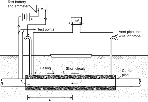

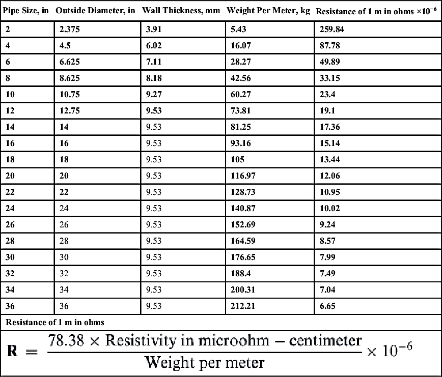


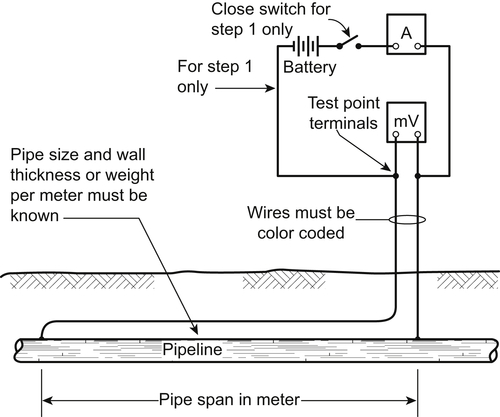
 (6.3)
(6.3)
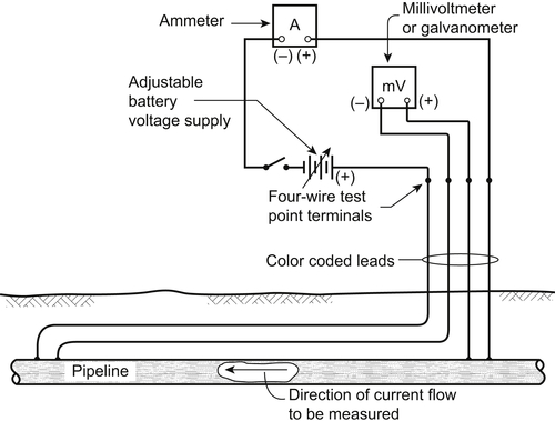
 (6.5)
(6.5)
 (6.23)