
Chapter 2. Process Heat Transfer
What You Will Learn
• The basics of process heat transfer
• The key relationships for designing and analyzing a heat exchanger
• Analysis of shell-and-tube heat exchangers
• Common correlations for heat transfer coefficients for single-phase and change-of-phase conditions
• The combination of these coefficients with appropriate resistances due to fouling and conduction to determine a single overall heat transfer coefficient
• Equations for extended heat transfer surfaces (fins) for common fin configurations
• Methods to design new heat exchangers
• Predicting the performance of existing exchangers
2.0 Introduction
The purpose of this chapter is to introduce the concepts needed to design and determine the performance of typical heat-exchange equipment (heat exchangers) used in the process industries. The emphasis is on shell-and-tube (S-T) exchanger design, but other exchanger types, such as air coolers, are mentioned. This chapter does not provide a comprehensive review of the processes of conduction, convection, and radiation, and the design and operation of fuel-fired boilers and fired heaters is not covered. Likewise, a comprehensive review of all heat transfer coefficients is not considered. The emphasis of this chapter is to present a set of useful working equations that can be used to design and evaluate the performance of heat exchangers. Multiple examples are included, and several comprehensive case studies for the design of heat exchangers are given.
2.1 Basic Heat-Exchanger Relationships
2.1.1 Countercurrent Flow
The flow configuration between process streams and/or utility streams is important in determining the correct driving force for heat transfer. The most common, idealized model is countercurrent flow, which is best illustrated in the sketch and the temperature-enthalpy diagram (T-Q diagram) shown in Figure 2.1.
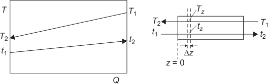
In Figure 2.1, subscripts 1 and 2 indicate inlet and outlet conditions, respectively. The temperatures of the two streams are identified by uppercase and lowercase letters (T and t). For the simple case shown in Figure 2.1, there are no phase changes in either stream. In addition, the specific heat capacities of both streams are assumed to be constant, which gives rise to the linear temperature profiles shown in Figure 2.1. The energy balances for both streams are
where capital letters are used for the hot stream and lowercase letters are used for the cold stream. The term Q is the total rate of heat transferred between streams (energy/time), ![]() and
and ![]() are the mass flowrates, and Cp and cp are the heat capacities of the streams. The streams are physically separated, usually by a metal wall, and heat is exchanged through this metal wall. The driving force for the heat exchange is, of course, the temperature difference (Tz − tz) between the two streams at the given location, z, in the heat exchanger. In general, this driving force changes throughout the exchanger, and some appropriate average should be used. In order to obtain a relationship between Q and the inlet and exit temperatures of each stream a simple differential balance can be written on an element of the heat exchanger, as illustrated in the right-hand sketch of Figure 2.1, to give
are the mass flowrates, and Cp and cp are the heat capacities of the streams. The streams are physically separated, usually by a metal wall, and heat is exchanged through this metal wall. The driving force for the heat exchange is, of course, the temperature difference (Tz − tz) between the two streams at the given location, z, in the heat exchanger. In general, this driving force changes throughout the exchanger, and some appropriate average should be used. In order to obtain a relationship between Q and the inlet and exit temperatures of each stream a simple differential balance can be written on an element of the heat exchanger, as illustrated in the right-hand sketch of Figure 2.1, to give
where (Tz − tz) = ΔTz. For many applications, the overall heat transfer coefficient U does not vary substantially with the location in the exchanger and thus Uz = U. Since the heat capacities of both streams are assumed to be constant, the temperature difference between the streams (Tz − tz) or ΔTz is also linear with respect to the amount of heat transferred, Q, as illustrated in Figure 2.2.

Figure 2.2 Temperature difference between streams, ΔT, as a function of the heat exchanged, Q, in a countercurrent heat exchanger
From Figure 2.2, it can be seen that

Substituting Equation (2.4) into Equation (2.3) and dropping the subscript z gives
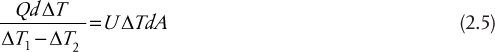
Integrating Equation (2.5) gives

or
where ΔTlm is known as the log-mean temperature difference, or LMTD, and is given as
For heat-exchanger design and performance calculations, the LMTD is the correct average temperature to use when the streams flow countercurrently, and Equation (2.8) is the design equation for heat exchangers.
Note: For the special case when the ![]() or when there are constant-pressure phase changes for both streams, then the ΔT between the hot and cold streams is constant throughout the heat exchanger; that is, the T-Q lines for both fluids are parallel. For such cases, the expression for LMTD gives 0/ln(1), which is indeterminate, but by using L’Hôpital’s rule, it can be shown that LMTD = ΔT. Since the LMTD is simply an average temperature difference between the streams, it should make sense that the average between identical temperature differences is just that temperature difference.
or when there are constant-pressure phase changes for both streams, then the ΔT between the hot and cold streams is constant throughout the heat exchanger; that is, the T-Q lines for both fluids are parallel. For such cases, the expression for LMTD gives 0/ln(1), which is indeterminate, but by using L’Hôpital’s rule, it can be shown that LMTD = ΔT. Since the LMTD is simply an average temperature difference between the streams, it should make sense that the average between identical temperature differences is just that temperature difference.
2.1.2 Cocurrent Flow
An alternative flow pattern in heat exchangers is cocurrent flow, which is illustrated in the sketch and T-Q diagram shown in Figure 2.3.
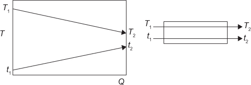
A similar analysis to that given for the countercurrent exchanger could be carried out for the cocurrent configuration and would result in the same Equation (2.5). However, now ΔT1 = (T1− t1) and ΔT2 = T2− t2. The cocurrent configuration is less efficient in terms of heat exchange for two reasons. First, the average driving force is smaller than for countercurrent operation; therefore, the heat-exchange area for a given Q will be higher for cocurrent flow than for countercurrent flow. Second, the limiting temperature that either stream can reach is the exit temperature of the other stream, whereas for countercurrent operation, the limiting exit temperature is the inlet temperature of the other stream. Examples 2.1 and 2.2 illustrate these differences.
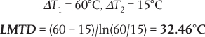
A gas is to be cooled from 100°C to 45°C using cooling water that enters the heat exchanger at 30°C and leaves at 40°C. What is the LMTD for the heat exchanger if the flow of the streams is
a. countercurrent?
b. cocurrent?
c. How much more heat-exchange area would be required for the cocurrent exchanger compared to the countercurrent exchanger?
Solution
a. For countercurrent flow, the T-Q diagram is shown in Figure E2.1A.

Figure E2.1A T-Q diagram for countercurrent flow in Example 2.1
b. For cocurrent flow, the T-Q diagram is shown in Figure E2.1B.
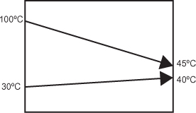
Figure E2.1B T-Q diagram for cocurrent flow in Example 2.1

Thus the cocurrent exchanger area would be 31.8% larger than the countercurrent exchanger area for the same heat duty.
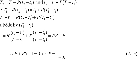
For the streams and flow configurations used in Example 2.1, what is the lowest temperature to which the gas stream can be cooled assuming the cooling water must leave the exchanger at 40°C?
Solution
The limiting condition for each heat-exchanger configuration is given when the exit gas stream is at the same temperature as the cooling water temperature, this situation is shown for countercurrent and cocurrent flows in Figure E2.2 (a) and (b), respectively.

This gives
2.1.3 Streams with Phase Changes
Often in chemical processes, heat exchangers are used to boil or condense streams. When there is a change of phase in either or both streams, the temperature-enthalpy diagrams for heat exchangers look different from those shown in Section 2.1.1. Some examples are illustrated in Figure 2.4. In Figure 2.4, the phase change occurs at constant temperature and nearly constant pressure, and there is no subcooling or superheating of streams. Therefore, one fluid is either simply boiling or condensing while the other fluid does not undergo a phase change.

Figure 2.4 T-Q diagrams for (a) Stream 1 cooling and Stream 2 boiling, (b) Stream 1 condensing and Stream 2 heating, (c) Stream 1 condensing and Stream 2 boiling
For all these cases, the LMTD should be used as the appropriate temperature driving force in heat-exchanger calculations. More complicated examples exist when both temperature and phase changes for one or both fluids occur within the same heat exchanger. This results in sensible heat changes (![]() ) and phase changes (
) and phase changes (![]() ) occurring within the same heat exchanger. For example, Figure 2.5 illustrates the case when Stream 2 is a subcooled liquid that is heated to saturation, boiled, and then the vapor is superheated using a superheated vapor (Stream 1) that cools, condenses, and subcools.
) occurring within the same heat exchanger. For example, Figure 2.5 illustrates the case when Stream 2 is a subcooled liquid that is heated to saturation, boiled, and then the vapor is superheated using a superheated vapor (Stream 1) that cools, condenses, and subcools.

Figure 2.5 T-Q diagram in which Stream 1 enters as a superheated vapor and is cooled to saturation (a1 to a2), condenses (a2 to a3), and then is subcooled (a3 to a4) and leaves as a subcooled liquid (a4) while transferring heat to Stream 2 that enters as a subcooled liquid and is heated to saturation (b1 to b2), vaporizes (b2 to b3), and is then superheated (b3 to b4) and leaves as a superheated vapor (b4) (the dotted lines between a1 and a4 and b1 and b4 should not be used to determine the LMTD)
From Figure 2.5, it should be clear that using a single LMTD (shown by the dotted lines drawn between the end-point temperatures) based on the conditions of the streams entering and leaving the heat exchanger does not provide a realistic or accurate estimate of the correct average driving force within the heat exchanger. In cases such as these, it is necessary to divide the heat exchanger into sections in which the T versus Q line is a single straight line segment for each fluid in each section. For the case illustrated in Figure 2.5, this would result in five separate sections, known as zones, labeled A through E in the figure. The design (and performance) of the heat exchanger would then follow a “zoned analysis” that would consider each section or zone (A–E in Figure 2.5) separately.
2.1.4 Nonlinear Q versus T Curves
In certain cases, most often when there is a large temperature change for a fluid in a heat exchanger, the specific heat capacity of the fluid may change significantly, and the T-Q line for a stream (or both streams) is curved, as shown in Figure 2.6. This situation can also occur when partial condensation occurs in a stream containing condensable and noncondensable components; however, this situation is far more complicated and must be considered as a separate case (see Section 2.1.5).

Figure 2.7 T-Q diagram for an exchanger with a variable specific heat, where Ti and ti are intermediate temperatures used in the linear approximation of the temperature profile
Comparing Figure 2.6 and the analysis carried out in Section 2.1.1, it should be clear that since the T-Q lines for at least one of the streams is not straight, the integration of Equation (2.3) will no longer yield the LMTD and Equation (2.7). For these cases, the usual practice is to integrate Equation (2.3) numerically to give the appropriate form of Equation (2.8).
An alternative method is to approximate the curved T-Q line as straight line segments, and the LMTD for each segment can then be found, similar to a zoned analysis. Figure 2.7 illustrates this method.
2.1.5 Overall Heat Transfer Coefficient, U, Varies along the Exchanger
In the derivation of LMTD given in Section 2.1.1, it was assumed that the overall heat transfer coefficient did not vary within the heat exchanger. Often this assumption is very good. However, for the case when streams undergo large temperature changes, the physical properties used to estimate film heat transfer coefficients, especially liquid viscosity, may change greatly. For this case, the analysis to determine the required heat transfer area becomes complex because the variation in U must be included in the integration of Equation (2.3). For the case when the change in U is linear or close to linear with the amount of heat transferred, Q, a modification of Equations (2.8) and (2.9) can be made:

where the term ![]() is the logarithmic mean of the product of U and ΔT. Example 2.3 illustrates the use of this equation.
is the logarithmic mean of the product of U and ΔT. Example 2.3 illustrates the use of this equation.
Low-pressure steam at 160°C is used to heat very viscous oil from 30°C to 65°C in a heat exchanger located at the inlet to a pump. The amount of energy needed to heat the oil is 2.65 GJ/h. Over the temperature range of the oil, the physical and transport properties of the oil are all constant except for the viscosity, which decreases significantly as the oil is heated. Using this information, calculations show that the overall heat transfer coefficients at the oil inlet and outlet are 245 and 390 W/m2/K, respectively. For this exchanger, draw the T-Q diagram and calculate the heat transfer area required in the heat exchanger.
Solution
The information in the problem statement is represented in Figure E2.3.
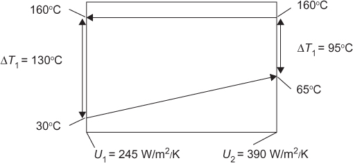
Figure E2.3 Variation of temperature differences and overall heat transfer coefficients over the heat exchanger
Using Equation (2.10),

For the case of partial condensation from a gas stream containing noncondensables, the situation is even more complex, because the temperature driving force and U may both vary nonlinearly with Q. Additionally, the mass transfer of the condensable component through the noncondensable component to reach the cold surface must be considered. Such situations require numerical solutions that include the changing physical properties, film heat and mass transfer coefficients, and temperature driving forces throughout the heat-exchange equipment. Many commercial software vendors, including Heat Transfer Research, Inc. (HTRI), Aspen Technology, Inc., Chemstations, and others, provide programs to perform these calculations.
2.2 Heat-Exchange Equipment Design and Characteristics
2.2.1 Shell-and-Tube Heat Exchangers
Throughout this chapter, many references are made to S-T heat exchangers. These exchangers are the workhorse of the process industry, and an enormous amount of literature is available about the thermal and mechanical design of this type of equipment. Many of the mechanical considerations are set forth in the Standards of the Tubular Exchanger Manufacturers Association (Tubular Exchanger Manufacturers Association [TEMA], 2013). A brief summary of the key design considerations are given here followed by a list of heuristics for choosing which fluid should be placed in the shell or tube side of the heat exchanger. The main components of an S-T exchanger are:
• Shell and shell cover
• Tubes and tubesheet
• Channel and channel cover
• Baffles
• Inlet and outlet nozzles
A good review of each of these components is given by Mukherjee (1998), and a summary of the results of this work are presented in the next section. The TEMA designations for S-T heat exchangers are given in Figure 2.8, the notation for several examples of S-T exchangers are given in Figure 2.9, and some standard designs are given in Figure 2.10.
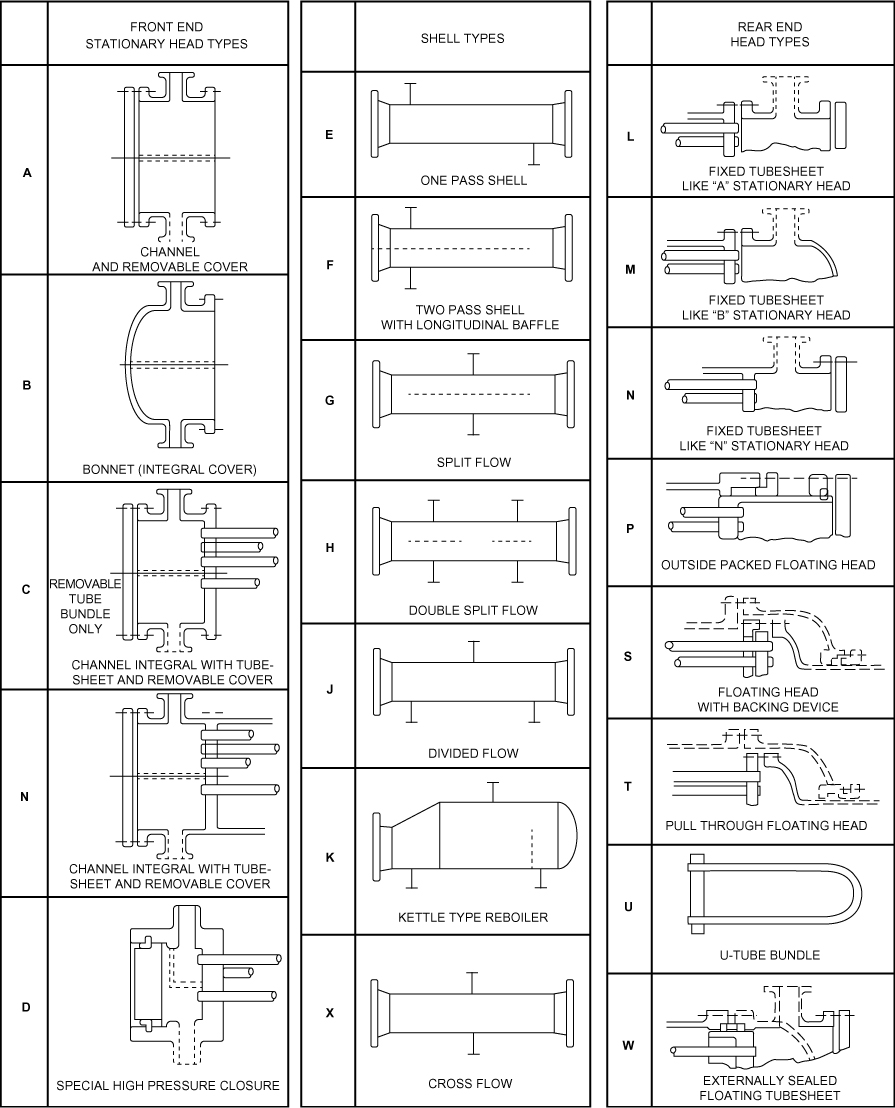
Figure 2.8 TEMA designations for shell-and-tube heat exchangers (Courtesy of Tubular Exchanger Manufacturers Association, Inc. [TEMA, 2013])

Figure 2.9 Notation for shell-and-tube heat exchangers (Courtesy of Tubular Exchanger Manufacturers Association, Inc. [TEMA, 2013])


Figure 2.10 Some standard shell-and-tube heat exchanger designs (Courtesy of Tubular Exchanger Manufacturers Association, Inc. [TEMA, 2013])
2.2.1.1 Shell Configurations
There are essentially seven types of shells, designated Types E, F, G, H, J, K, and X in Figure 2.8. The shell type essentially describes the flow pattern in the shell. The simplest and most common configuration is Type E, a one-pass shell, in which the shell-side fluid flows either from left to right (inlet on top left of shell) or from right to left (inlet at bottom right of shell). Two shell passes can be achieved in a single shell by providing a longitudinal baffle down the center of the shell (Type F) that extends to a point short of the tubesheet. If this type of exchanger has only two tube passes, then it is a true counter-current arrangement. Types G and H are characterized by a split flow on the shell side. For Type G, the feed and outlet nozzles are placed at the middle of the shell, and a longitudinal baffle, located at the centerline of the shell, diverts the fluid from the center to both ends and then back to the middle as it exits. The maximum tube length for this type of heat exchanger is ~3 m, since the tube cannot be supported and will lead to unacceptable tube vibration for longer unsupported tube lengths. For Type H, the shell-side fluid is split into two inlet nozzles, longitudinal baffles divert the flow to the left and right, and the flow reverses direction as it passes the baffles and flows back toward the two exit nozzles. This arrangement can be used if tube lengths longer than 3 m are desired. Both Types G and H are used mainly for horizontal thermosiphon reboilers in which the driving force for circulation of the process fluid, which is partially vaporized, is due to the density difference between the liquid entering the reboiler and the two-phase mixture returning to the column. Type J is similar to Type H except there is only a single inlet nozzle and two outlets (1–2 Type J). Alternatively, there may be two inlets and one outlet (2–1 Type J). Type K is for kettle-type reboilers and is characterized by a flared shell that allows significant vapor disengaging space above the boiling liquid and also may contain an overflow weir that maintains a liquid level above the tube bundle. Type X is a cross-flow arrangement, usually containing multiple inlet distribution and collection nozzles inside the shell that approximates a cross-flow movement of the shell-side fluid. The pressure drop for the shell side of these exchangers is extremely low and is preferred for low-pressure and vacuum-vapor coolers and condensers.
2.2.1.2 Tubesheet and Tube Configurations
The tube-side and shell-side fluids are separated by tubesheets, one at either end of the heat exchanger, or, in the case when U-tubes are used, by a single tubesheet at one end of the exchanger. The tubesheet is generally a circular, flat piece of metal with holes drilled in it to accept the tube ends. Examples of tube connections are shown in Figure 2.11. Tubes may be attached to the tubesheet via a number of methods. For example, the tubesheet may be drilled, reamed, and machined with several grooves, with the tubes forced-fit and rolled into the grooves in the tubesheet, Figure 2.11(a). In addition, a strength- or seal-weld may be added, Figure 2.11(b). These welds provide complete separation between the two fluids (shell side and tube side) and ensure no intermixing of fluids occurs. For critical services, when it is vital to avoid intermixing of fluids because of violent cross-reaction and/or degradation of valuable product, a double tubesheet may be employed, Figure 2.11(c). The gap between the tubesheets would typically be vented and monitored for any leaks.

The arrangement or layout of tubes in an S-T exchanger is determined by the rotation or orientation of the tubes relative to the shell-side fluid, the spacing between the tube centers (the tube pitch), and the layout pattern (triangular or square). Some variations of these three factors are illustrated in Figure 2.12. In general, a given shell diameter accommodates more tubes if a triangular arrangement is used (Figure 2.12[c] and 2.12[d]), and this leads to more turbulence on the shell side and a correspondingly higher shell-side heat transfer coefficient. On the down side, when the typical tube pitch of 1.25 times the tube outer diameter is used, a triangular arrangement will not permit the mechanical cleaning of the tubes, because there are no access lanes between the tubes to allow for a brush or similar device to clean the accumulated scale from the outside surfaces of the tubes. Mechanical cleaning on the shell side using a triangular arrangement of tubes is possible if a larger tube pitch is used, but this requires a larger shell diameter and greater expense. When mechanical cleaning is desired on the shell side, a square or rotated square pitch is preferred.
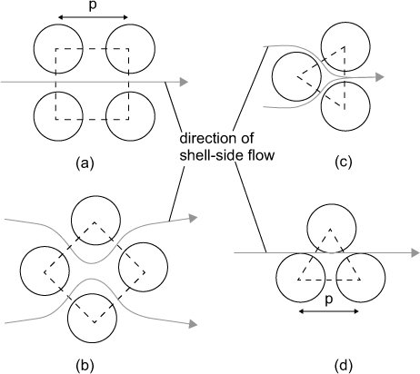
Figure 2.12 Layout patterns for tubes (a) square pitch, (b) rotated square pitch, (c) triangular pitch, and (d) rotated triangular pitch

2.2.1.3 Fixed Tubesheet and Floating Tubesheet (Head) Designs
For a “standard” 1–2, S-T heat exchanger, the tubesheet at the front end of the exchanger, which contains the feed and discharge nozzles (left column of Figure 2.8), is fixed or anchored to the exchanger. This is referred to as a stationary head. For the case when the tubesheet at the other end of the exchanger is also fixed, as illustrated in Types L, M, and N in Figure 2.8, the exchanger is referred to as a fixed-tubesheet design. Since the average temperatures on the shell side and tube side will be different, thermal expansion of the tubes and shell will also be different, and this differential expansion will cause mechanical stress at the points where the tubes and shells are connected or anchored. For small differences between the average shell- and tube-side temperatures, this mechanical stress is not excessive, and no damage to the exchanger will result. However, as the average temperature difference between the two fluids in the exchanger becomes larger, the differential expansion becomes excessive and could cause buckling and failure for a fixed tubesheet exchanger. To alleviate this problem, a floating head or floating tubesheet is used, as shown in Figure 2.8 (types P, S, T, and W). It should also be noted that the use of U-tubes (Type U) eliminates the use of a second tubesheet and, therefore, eliminates any problems associated with differential thermal expansion. However, it is difficult to clean the “U-bend” in these tubes mechanically, so the use of U-tubes should be avoided when the tube-side fluid fouls.
2.2.1.4 Shell-and-Tube Partitions
The standard 1–2, S-T design can be stacked to form any combination of N-2N shell-tube designs. However, it is often economical to provide multiple tube-pass and shell-pass configurations in a single shell by the use of longitudinal partitions in the shell and by partitions in the tube channel or head. The longitudinal shell partitions are usually welded to the shell to avoid leakage and bypass. Likewise, the partitions in the tube channels at either end of the exchanger have plates welded in place to direct and redirect the tube-side flow through the multiple tube passes. In virtually all cases of S-T exchangers, one or more tube partitions will be present. Therefore, the arrangement of the tubes in the tube bundle along the line of the partition plates will result in areas without tubes, even when a shell-side partition is not used. This situation is shown in Figure 2.13.
2.2.1.5 Baffles
Shell-side baffles are used for two main reasons. First, they support the tubes at regular intervals, and the shorter the unsupported length of a tube, the less damage there is due to vibration. Second, the baffles direct the shell-side fluid back and forth over the tube bundle, and the perpendicular flow increases the shell-side heat transfer coefficient. There are essentially two types of baffles (plate and rod types), and they are available in several different arrangements. Figure 2.14 shows the three common arrangements for plate baffles and the notation used to describe the baffle arrangements. The baffle-cut is the fraction of the diameter of the baffle plate that is totally open to flow. The baffle cut is usually expressed as a percentage, such as 20%. The maximum range of values for baffle cut is between 15% and 45%, although a narrower range of 20% to 35% is strongly recommended by Mukherjee (1998). Other arrangements of plate baffles are also possible, such as triple segmented baffles and baffles without tubes in the baffle windows. For rod-type baffles, the tubes are held in place by a series of rods placed at right angles to other rods and the tubes. One arrangement is shown in Figure 2.15. The advantages of rod baffles are their low pressure drop and reduction in tube vibrations. For rod-type baffles, the direction of flow is essentially parallel to the tube bundle. The shell-side fluid flows through the gaps between the rods and tubes, which promotes local turbulence and good heat transfer while reducing the shell-side pressure drop.
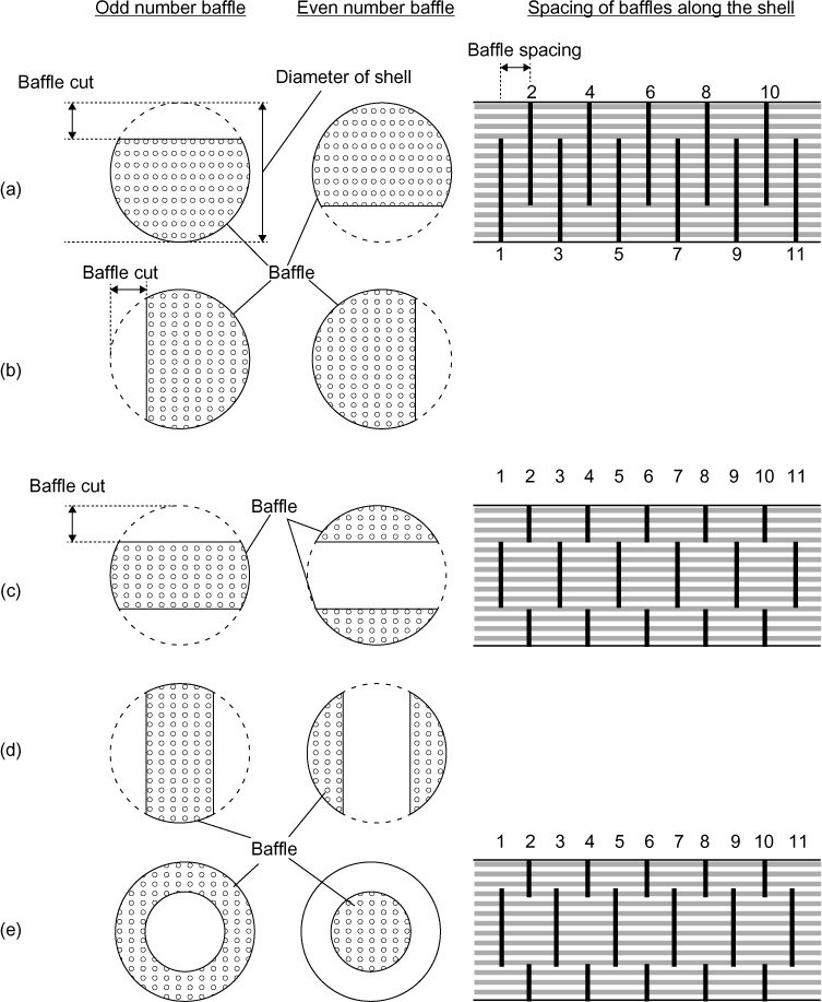
Figure 2.14 Typical arrangements for plate baffles: (a) single segmented baffle, horizontal arrangement; (b) single segmented baffle, vertical arrangement; (c) double segmented baffle, horizontal arrangement; (d) double segmented baffle, vertical arrangement; (e) disk and donut baffles
2.2.1.6 Shell-Side Flow Patterns
From the previous section, it is clear that baffles are usually used to promote the ordered movement of shell-side fluid from the inlet to the outlet. The actual flow pattern that the fluid takes in a design using plate baffles is very complicated, because, in addition to the intended cross flow movement of the shell-side fluid, there are multiple alternative leakage paths that allow fluid to bypass the intended flow direction. An analysis of the flow patterns in plate baffle exchangers was made by Tinker (1958), who identified four leakage or bypass streams in addition to the main cross-flow stream. The main and desired flow direction for the shell-side fluid is shown as B in Figure 2.16. Stream B moves as a cross-flow stream across the tube bundle and then reverses at the shell wall and flows back across the tube bundle before reversing at the opposite shell wall and so on. This movement provides very efficient heat transfer. Accompanying this flow are four alternative streams (A, C, E, and F), which do not follow the desired flow pattern. Flow pattern A is caused by the clearance between the baffle plates and the tubes that allows fluid to pass between the gaps in the baffle plate. Flow pattern C is a bundle bypass stream, which does not fully penetrate the depth of the tube bundle but rather slipstreams around the next baffle. Flow pattern E is caused by fluid flowing parallel to the tube bundle at the walls of the shell. This fluid essentially provides little or no heat transfer between the shell and tube fluids. The final flow pattern, F, is a longitudinal flow created by areas in the tube bundles that have a disrupted tube pattern. Such areas occur when there are shell-side partitions or tube-side partitions. For the case when there is a shell-side partition, a gap exists next to the partition that has fewer tubes in it compared with the main tube bundle. Even for the case when there is no shell-side partition, the arrangement of tubes to accommodate the number of tube passes causes a disruption in the pattern of tubes in the shell giving rise to by-passing lanes (see Figure 2.13). In both these cases, a low resistance path for the shell-side fluid exists, creating a bypass stream, F. Figure 2.17 shows the effect that baffle cut has on side flow patterns. If the baffle cut is too large, then significant shortcutting of fluid (Flow Pattern C in Figure 2.16) occurs that lowers the heat transfer efficiency. As the baffle cut decreases, the shell-side pressure drop increases significantly. As stated previously, the recommended baffle (BC) cut is between 20% and 35%.

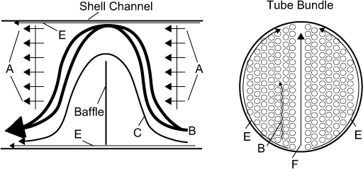
Figure 2.16 Flow patterns on shell-side of an S-T exchanger: B, desired; A, baffle plate leakage; C, flow short circuiting around baffle; E, flow short circuiting around shell wall; F, flow short circuiting through tube bundle (Adapted from Tinker [1958])
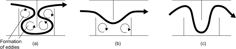
Figure 2.17 The effect of baffle-cut on the flow pattern of shell-side fluid: (a) baffle-cut too small causing high pressure drop, (b) baffle-cut too large giving significant flow bypassing and poor penetration of tube bundle, (c) baffle-cut just right showing good penetration of shell-side flow through tube bundle (Adapted from Mukherjee [1998])
2.2.1.7 Heuristics for Shell-and-Tube Exchanger Designs
The following is a list of heuristics for the design of S-T heat exchangers that is modified from Bell and Mueller (2014). Like any set of heuristics, these should be used as guidelines and not as immutable laws. Some heuristics may seem to be contradictory, and the final choice is often a compromise between conflicting phenomena, with the deciding factor being which design is the least expensive.
Choice of Tube-Side Fluid
• If one stream has a much lower film coefficient that the other, the lower coefficient stream should be placed in the shell so that extended surfaces (fins) can be added to the outside of the tubes to increase the surface area (see Section 2.6). Therefore, if a gas and a liquid are to exchange heat, the gas would normally go on the shell side. For high- and low-viscosity liquids, the low-viscosity fluid is normally placed in the tubes.
• If one fluid is highly corrosive (compared to the other), this fluid should be placed in the tubes. This heuristic is due to the corrosive fluid needing to be in contact with a corrosion-resistant alloy, which is usually expensive. It makes the best economic sense to have the tubes (and connecting piping) made from this alloy. On the other hand, the shell (and baffles and tie rods, etc.) can be made out of a less expensive material (like carbon steel) that is only in contact with the shell-side (less corrosive) fluid.
• If the temperature and pressure conditions for one of the fluids require the use of specialty alloys, that fluid is placed in the tubes for the same reasons given for highly corrosive fluids.
• When one fluid is at much higher pressure than the other fluid, that fluid is placed in the tubes. Since higher pressure requires thicker walls, it makes sense to place the high-pressure fluid inside the tubes, while the shell can be designed for the lower-pressure fluid.
• If one fluid causes severe fouling or scaling, that fluid is placed in the tubes, but a U-tube (Type U) design is not used. Since straight tubes can be mechanically cleaned relatively easily, it makes sense to put the fouling fluid in the tubes.
Choice of Shell Type
• Fixed tubesheet arrangements are not designed to be able to relieve thermally induced stresses. One heuristic is to use fixed tubesheet exchangers only when the inlet temperatures of the two streams differ by less than 55°C (100°F).
• Fixed tubesheet exchangers have been used for temperature differences up to 110°C (200°F) with rolled expansion joints for moderate pressures in the shell (<10 bar).
• U-tube bundles provide a comprehensive solution to the thermal stress problem on the tube side, because they contract and expand independently of the shell, but tubesheet stresses still exist.
• If one fluid is very viscous, this fluid should be placed on the shell side, provided that by doing so the fluid is in the turbulent regime (Res > 100). If turbulent flow conditions cannot be achieved in the shell, the viscous fluid should be placed in the tubes.
• If one fluid requires a low-pressure drop through the exchanger, this fluid is placed on the shell side of the exchanger. In general, the shell-side pressure drop is lower than the tube-side pressure drop. In addition, as discussed in Section 2.2.1.1, many different shell configurations are available that lower the shell-side pressure drop.
2.3 LMTD Correction Factor for Multiple Shell and Tube Passes
2.3.1 Background
In the previous sections, the ideal case of pure countercurrent flow and the configuration of typical S-T heat exchangers were investigated. For nonreacting systems, pure countercurrent flow is the best flow configuration (the configuration that requires the smallest heat-exchange area) for a given system. In practice, exchangers with pure countercurrent flow are not the usual choice. For reasons of compactness and cost, heat exchangers are configured with flow patterns that usually fall somewhere between the extremes of pure countercurrent and pure cocurrent flow.
To account for flow patterns that are not purely countercurrent, Equation (2.8) can be rewritten to include an LMTD correction factor, Fy, where the subscript refers to a type of flow such as cocurrent or cross-current or to the type of heat exchanger being used. Thus, the generalized working design equation for exchangers becomes:
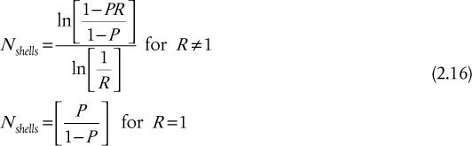
By convention, the LMTD for pure countercurrent flow is taken as the reference configuration, and the correction factor, Fy, is always the correction relative to pure countercurrent flow. In this way, Fy is always less than or equal to 1.0. For pure cocurrent flow, the LMTD correction factor, Fcocurrent, is given by

where P is the ratio of the temperature change of the tube-side stream to the maximum temperature difference in the exchanger and R is the ratio of heat capacities of the tube-side to shell-side streams,

Revisit Example 2.1 and show that the same answer to Part (c) can be found using Equation (2.12).
Solution
t1 = 30°C, t2 = 40°C, T1 = 100°C, T2 = 45°C
For cocurrent flow, P = (40 − 30)/(100 − 30) = 10/70 = 0.1429 and R = (100 − 45)/(40 − 30) = 5.5. Substituting into Equation (2.12),

Applying Equation (2.11) to the cocurrent and countercurrent exchangers and taking ratios give
This is the same result as given in Part (c) of Example 2.1. It should be noted that the choice of which stream to assign T and t is not important, and this point will be illustrated Example 2.5.
In the process industries, the workhorse of industrial heat exchangers is the S-T design. Many of the important design issues for these heat exchangers were covered in Section 2.2. However, in the next section, the effect of different, nonideal flow patterns on the LMTD correction factor (Fy) is covered.
2.3.2 Basic Configuration of a Single-Shell-Pass, Double-Tube-Pass (1–2) Exchanger
As pointed out in Section 2.2, the most common form of heat exchanger in the process industries is the S-T heat exchanger. The most common form of S-T exchanger is the single-shell-pass, two-tube-pass or 1–2 design, which is illustrated in Figure 2.18.
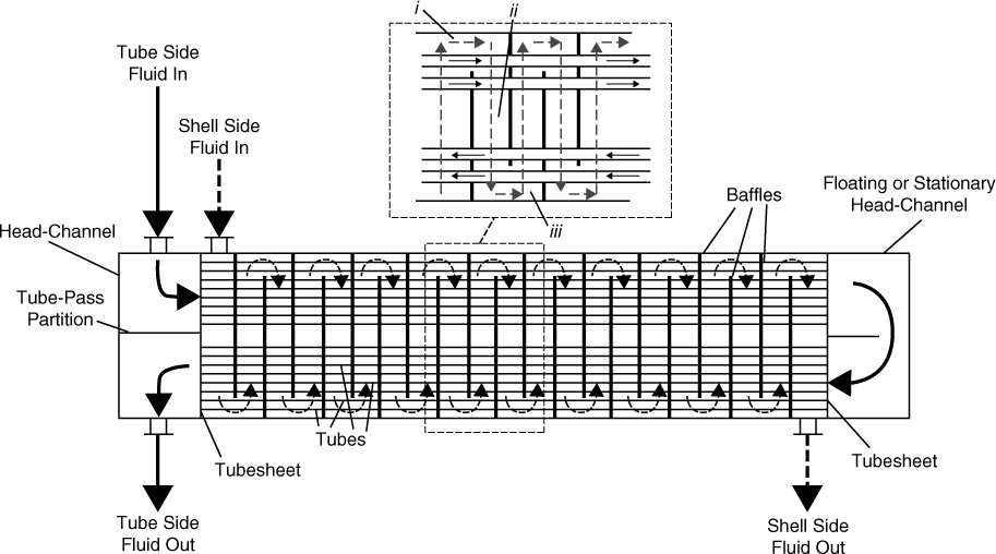
Figure 2.18 Flow configuration for a 1–2, S-T heat exchanger—solid lines with arrows show flow path for tube-side fluid, and dotted lines with arrow show flow path for shell-side fluid
Figure 2.18 is a schematic diagram illustrating the flow pattern for a 1–2, S-T heat exchanger. Many of the technical details of S-T heat exchangers are covered in Section 2.2, but a further, brief description of the fluid flow paths is given here. Referring to Figure 2.18, the tube-side fluid enters from the top of the diagram and passes into a head-channel. The fluid then flows horizontally (from left to right) through a series of parallel tubes into a second head-channel on the right of the diagram. The tube-side stream then reverses direction and passes from right to left through the bottom set of parallel tubes into the left-hand head-channel where it finally leaves the heat exchanger. The shell-side fluid enters the shell, which is separated from the two head-channels by a tubesheet at either end of the exchanger. The shell-side fluid passes from left to right in the shell and is guided by a set of baffles that direct the flow. This fluid finally leaves the shell at the bottom right in the diagram. An insert is shown at the top of Figure 2.18 that shows in more detail the flow patterns of the different streams. The insert identifies three regions (labeled i, ii, and iii). In Region i, the shell-side and tube-side fluids flow cocurrently with each other. In Region ii, the shell-side fluid flows perpendicular or cross-currently with the fluid in the tubes. Finally, in Region iii, the shell- and tube-side fluids flow counter-current to one another. From this description, it should be clear that the flow pattern in this type of heat exchanger does not fit either the countercurrent or cocurrent models described previously.
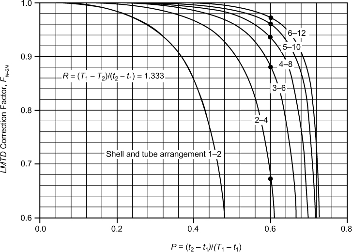
Despite the apparently complicated flow pattern shown in Figure 2.18, it has been shown by Bowman, Mueller, and Nagle (1940) that the flow pattern is closely approximated by half the exchanger with cocurrent flow (top half of tubes in Figure 2.18) and the other half with counter-current flow. With this assumption, an analytical expression for F1–2 can be found, and is given as Equation (2.13) and Figure 2.19.
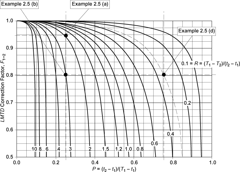
Figure 2.19 LMTD correction factor, F1–2, for a 1–2, S-T heat exchanger (this figure is also good for one shell pass and any even number of tube passes, i.e., F1–4, F1–6, F1–8, etc.).
Figure 2.19 illustrates the correction factor, F1–2, as a function of P and R for a 1–2, S-T exchanger. It should be noted that the correction factor for a 1–2, S-T exchanger is essentially the same (within 1% to 2%) for a single shell pass with any number of even tube passes, and the results from Equation (2.13) and Figure 2.19 may be used. Therefore, F1–2 = F1–4 = F1–6 = F1–8, and so on.
From Figure 2.19, it should be clear that for any given value of R, there exists a maximum value of P, Pmax. The value of Pmax is given by Equation (2.14):
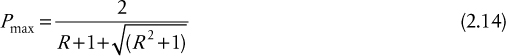
For values of P > Pmax no solution to Equation (2.13) exists, or to put it another way, a 1–2, S-T exchanger cannot always be used to make the temperature of the streams change as desired. The uses of the LMTD correction factor, Figure 2.19, and the limitations of 1–2, S-T exchangers are illustrated in Example 2.5.
a. A 1–2, S-T heat exchanger is used to cool a process stream from 70°C to 50°C using cooling water at 30°C heated to 40°C. For this heat exchanger, determine the value of F1–2.
b. Repeat this calculation, using the same cooling water temperatures for the case when the exit process temperature is 40°C.
c. Repeat this calculation, using the same cooling water temperatures for the case when the exit process temperature is 35°C.
d. Repeat Part (b) but switch the tube and shell side fluids.
Solution
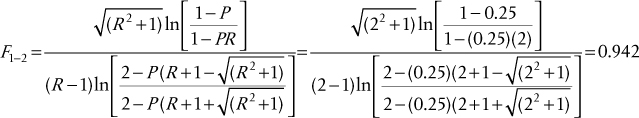
a. P = (t2 − t1)/(T1 − t1) = (40 − 30)/(70 − 30) = 0.25
R = (T1 − T2)/(t2 − t1) = (70 − 50)/(40 − 30) = 2.0
From Figure 2.19, values for P and R are shown as dotted lines, and F1–2 = 0.942. Alternatively, using Equation (2.13),
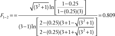
b. P = (t2 − t1)/(T1 − t1) = (40 − 30)/(70 − 30) = 0.25
R = (T1 − T2)/(t2 − t1) = (70 − 40)/(40 − 30) = 3.0
From Figure 2.19, F1–2 = 0.81 and using Equation (2.13),
c. P = (t2 − t1)/(T1 − t1) = (40 − 30)/(70 − 30) = 0.25
R = (T1 − T2)/(t2 − t1) = (70 − 35)/(40 − 30) = 3.5
From Figure 2.19 or using Equation (2.11), there is no solution; that is, it is not possible to design a 1–2, S-T exchanger for this situation.
The situation can be verified by applying Equation (2.14):
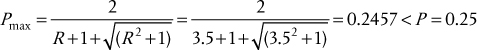
This confirms that only values of P < Pmax result in feasible solutions.
d. P = (t2 − t1)/(T1 − t1) = (40 − 70)/(30 − 70) = 0.75
R = (T1 − T2)/(t2 − t1) = (30 − 40)/(40 − 70) = 0.333 From Figure 2.19, F1–2 = 0.81 and using Equation (2.13),

The result is the same as in Part (b).
Two important conclusions can be drawn from Example 2.5. First, by comparing the results for Parts (b) and (d), it can be seen that it does not matter what stream is chosen for the shell-side or tube-side fluid. Equation (2.13) and Figure 2.19 are essentially symmetrical in R and P, so that the choice of which fluid to put in the shell and which to put in the tubes does not affect the result and value of F1–2. Other factors do affect which fluid goes where, but these were covered in Section 2.2.1.5. Secondly, it was seen that, as the exit temperature of the process fluid decreased, F1–2 started to decrease. Specifically, when the outlet temperature of the hot stream drops below the outlet temperature of the cold stream (T2 < t2), the efficiency drops very rapidly, and for Part (c) no solution existed. These results can be explained by the fact that as the temperature between the hot exit and cold exit streams approaches zero, the efficiency of the 1–2, S-T design is reduced significantly. This effect is illustrated in Figure 2.20. For pure cocurrent flow, the highest temperature to which the cold stream can be heated is equal to the hot stream exit temperature. However, in a 1–2, S-T exchanger only half of the flow is cocurrent, so not surprisingly, the efficiency (F1–2) of the heat exchanger starts to decrease rapidly when this condition is reached. Heat exchangers with multiple shell passes more closely mimic pure countercurrent flow, and these are covered next.
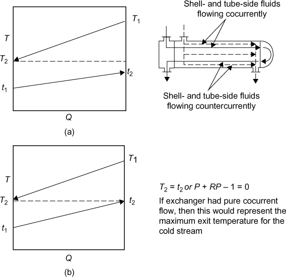
Figure 2.20 T-Q profiles in 1–2, S-T exchanger: (a) satisfactory temperature approach, (b) exit temperatures of both fluids are equal (F1–2 ≅ 0.8)
2.3.3 Multiple Shell-and-Tube-Pass Exchangers
For a 1–2, S-T exchanger with the condition T2 = t2, using the relationships between P and R as follows,
The line representing Equation (2.15) can be approximated by the condition F1–2 = 0.8 on Figure 2.19. The usual design criterion for exchanger design is to limit the LMTD correction factor to a value ≥ 0.8. If the condition of F = 0.8 is taken as the reasonable practical limit of operation of a 1–2, S-T exchanger, the number of shells needed for any design can be calculated graphically using a McCabe-Thiele–type construction, illustrated in Figure 2.21. The analytical expression for the number of shells using this criterion if the specific heats of hot and cold streams are constant (lines on the T-Q diagram are straight) is given by

Figure 2.21 McCabe-Thiele–type construction for estimating the number of shell passes for an S-T heat exchanger and the arrangement of three 1–2, S-T exchangers to give a 3–6 S-T configuration
Analytical expressions for the LMTD correction factor, F, for higher shell and tube passes exist, and many of these are given by Bowman et al. (1940). For a 2–4, S-T exchanger, Equation (2.17) applies (this expression can also be used for a 2–4N, S-T exchanger, where N = 1, 2, 3,...):
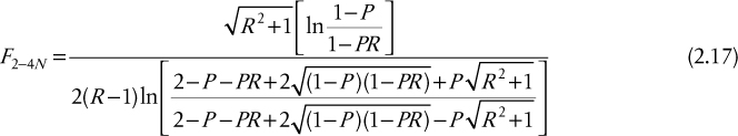
For the case when R = 1, Equation (2.17) reduces to Equation (2.18):

For higher shell passes, the analytical expressions become more complicated. However, Bowman (1936) has shown that for any given values of F and R, the value of P for an exchanger with N shell-side and 2N tube-side passes can be related to P for a 1–2, S-T exchanger through Equation (2.19):

Equation (2.19) was used to generate the LMTD correction factors for 3–6, 4–8, 5–10, and 6–12 S-T exchangers, and the results are presented in Appendix 2.A. LMTD correction factors for many types of heat exchanger can also be found at http://checalc.com/solved/LMTD_Chart.html. It is observed that as the number of shell passes increases, the curve for the same value of R moves up, resulting in a higher F value. Example 2.6 illustrates the use of multiple shell heat exchangers.
a. How many shell passes would be needed to cool a heavy oil stream from 230°C to 150°C using another process stream that is heated from 130°C to 190°C?
b. What is the LMTD correction factor for this arrangement?
a. P = (t2 − t1)/(T1 − t1) = (190 − 130)/(230 − 130) = 60/100 = 0.60
R = (T1 − T2)/(t2 − t1) = (230 − 150)/(190 − 130) = 80/60 = 1.333
Applying Equation (2.16),
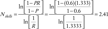
Rounding up, to Nshells = 3 means that a 3–6, S-T exchanger is required.
b. From Figure A.3, F3–6 = 0.88 this value is >0.8, which satisfies the criterion for acceptable efficiency. From Figure A.2, F2–4 = 0.67, which is below the acceptable limit of 0.8. It should be noted that 4–8, 5–10, and higher numbers of S-T passes would all be acceptable designs, but the complexity and cost of the exchanger increases with the addition of shell passes; therefore, the design with the fewest number of shell passes should be chosen. The effect of the number of shell and tube passes for this example is further illustrated in Figure E2.6 where the curves for different S-T configurations for R = 1.33 are plotted.
2.3.4 Cross-Flow Exchangers
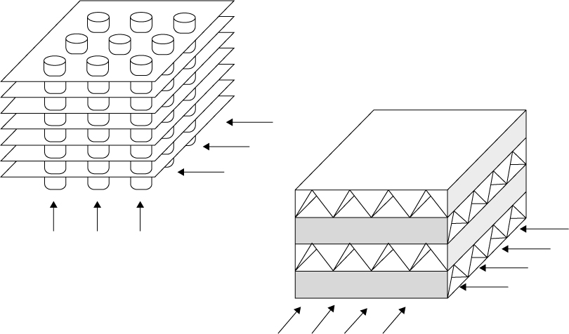
For some heat exchangers, the two fluids exchanging energy flow are at right angles to each other. This flow pattern is termed cross-flow, and there are several important examples of this type of flow pattern in commercial heat exchangers. One example is the plate-and-frame heat exchanger, another example is the air-cooled heat exchanger, where air flows perpendicular to a set of finned tubes in which a liquid or condensing vapor flow. The purpose of finned tubes is to provide extended heat transfer surface to fluids with a low heat transfer coefficient; this topic is covered in detail in Section 2.6. A typical arrangement of an air cooler (sometimes termed a fin-fan) is illustrated in Figure 2.22. Other examples of cross-flow occur in gas-gas exchangers for which the film heat transfer coefficients for both gases are low. In such situations, each gas may pass through a channel that contains regular geometric fins, as shown in Figure 2.23. Values for the LMTD correction factor for one case of cross-flow is given in Appendix 2.A, Figure A.7. Other practical examples of cross-flow exchangers are car radiators and heat sinks on circuit boards and electronic power handling devices.

Figure 2.22 Schematic of an air cooler: Air is pulled up and across heat transfer tubes with external fins by an induction fan and hot fluid is transported through the tubes. The insert shows detail of the cross-flow pattern for the air and process fluid.
2.3.5 LMTD Correction and Phase Change
For cases when one or both fluids experience a phase change, with T-Q diagrams similar to those shown in Figure 2.4, the LMTD correction factor can be taken as unity; that is, no correction to the LMTD is needed. This should be apparent to the reader, since the fluid that is not changing phase is contacted everywhere with the phase change material that is at constant temperature (assuming constant pressure operation). Therefore, the flow pattern has no effect on the driving forces within the exchanger.
2.4 Overall Heat Transfer Coefficients—Resistances in Series
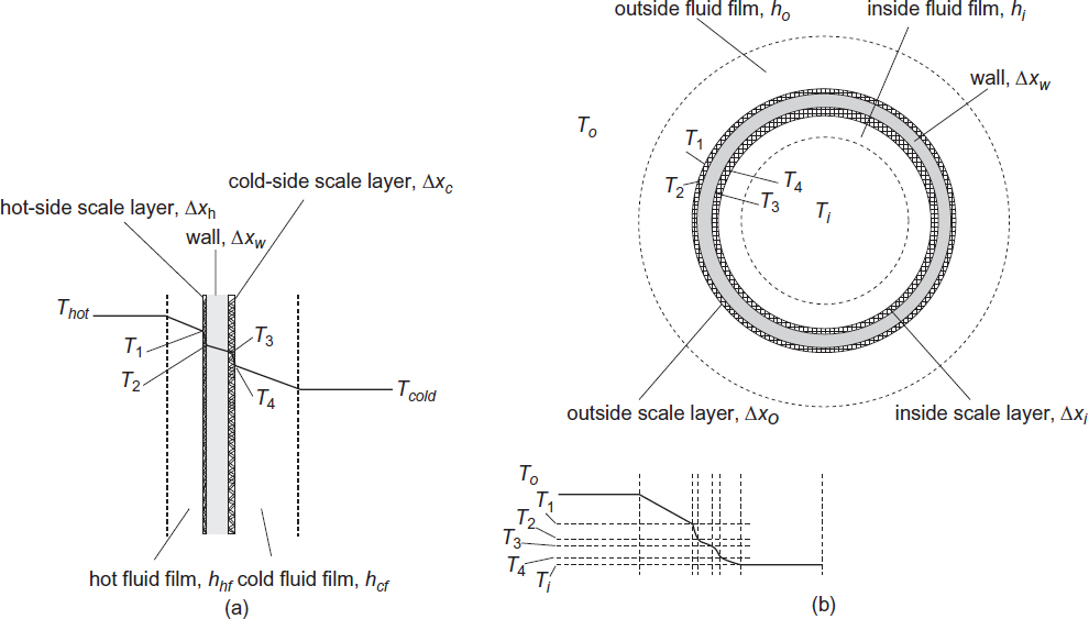
Up to this point, there has been no discussion on the value or determination of the overall heat transfer coefficient, U. U is the combination of several heat transfer resistances that act in series, and these resistances are illustrated in Figure 2.24 for both planar and circular geometries. In Figure 2.24(a), a wall is shown separating two fluids at different temperatures. For generality, it is assumed that the solid wall is composed of multiple layers. These layers might comprise a composite wall or a single wall with scale deposits on both sides. Either way, each layer acts as a separate resistance to heat transfer. In the case of a deposit of scale, the term fouling resistance is used. The heat transfer resistance between each fluid and the surface is given in terms of a film heat transfer coefficient (hi, ho), while the resistances of the solid layers are given in terms of their thermal conductivity (k) and thickness (Δx). In Figure 2.24(b), a similar situation is shown for cylindrical or tubular geometry.
For steady-state operations, the amount of heat transferred through each layer or resistance must the same. By writing the basic heat flux equation across each resistance and eliminating the intermediate temperatures, an overall expression of the heat transferred in terms of the bulk temperature driving force (which is used in the exchanger design equation) is obtained. This process is given for the planar geometry as follows:
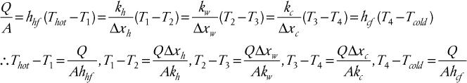
Adding all the left-hand sides together gives
where

For circular (tubular) geometry with a single wall and scale formation on the inner and outer surfaces, a similar analysis gives

where the subscripts o and i refer to the outside and inside of the tube, respectively, and the resistances due to fouling are given in terms of an effective fouling heat transfer resistance, Rfo = 1/hof and Rfi =1/hif, respectively. The form of Equation (2.21) differs from that derived for planar geometry, because for circular geometry, the cross-sectional area through which the heat flows changes from the outside to the inside of the tube. By eliminating the intermediate temperatures and rearranging, the following working equations for circular geometry can be derived:
where


where Di and Do are the inside and outside diameters of the tube (or pipe), respectively.
From Equations (2.23) and (2.24), it is clear that for circular geometry, the overall heat transfer coefficient must be defined with respect to a specific surface but that the product UA is the same no matter what surface is chosen; that is, UiAi = UoAo. It should also be noted that Equation (2.22) was derived for a specific location where ΔTBulk is known. If the temperature difference between fluids varies with location, as it would in most heat exchangers, then an appropriate average temperature difference should be used. The analysis given in Section 2.1 and all the limitations discussed in Section 2.1 still apply. Thus the general working equation for heat transfer between fluids exchanging heat through tube walls becomes
In summary, for heat transfer between fluid streams separated by a wall, the overall heat transfer resistance is a function of the two film heat transfer coefficients, two fouling resistances, and a resistance due to the wall. In the next section, typical correlations and values required to determine all these resistances are presented.
2.5 Estimation of Individual Heat Transfer Coefficients and Fouling Resistances
In Section 2.4, the terms needed to evaluate the overall heat transfer coefficient (Uo or Ui) were identified. In this section, correlations and other data for calculating each of these heat transfer resistances are presented.
2.5.1 Heat Transfer Resistances Due to Fouling
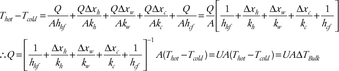
In designing heat exchangers, it is important to make allowance for the deposition of scale, that is, the process of fouling, on heat-exchanger surfaces and the subsequent reduction in overall heat transfer due to the fouling process. The a priori determination of fouling through some mechanistic model is not possible because of the highly complex nature of the fouling process. Moreover, fluctuations in process temperatures and other conditions (pH, total dissolved solids, etc.) due to abnormal plant operations may significantly increase the fouling process and are impossible to predict with any accuracy. With this in mind, the designer must resort to the use of typical fouling resistances for similar services (fluids) obtained through experience.
Fouling resistances for water and chemical process streams as suggested by TEMA (2013) are shown in Tables 2.1 and 2.2.
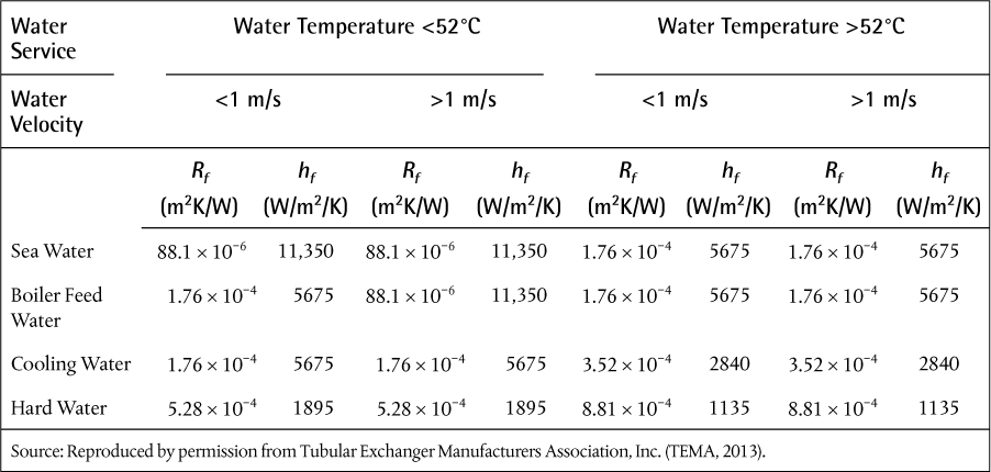
2.5.2 Thermal Conductivities of Common Metals and Tube Properties
Thermal conductivities for metals usually used as heat-exchanger tubes or in extended surface (compact) heat exchangers are given in Table 2.3. For low-temperature service such as cryogenic air separation, aluminum and stainless steel are the preferred materials of construction. It should be noted that the thermal conductivities of most metals do not vary widely over quite large temperature changes, and usually the resistance to conduction through the wall is not the limiting resistance, so minor changes in thermal conductivity rarely have a significant effect on heat-exchanger design or performance. From Table 2.3, it is clear that copper is the material with the highest thermal conductivity (lowest heat transfer resistance) and is favored as long as it is compatible with the fluids it contacts. Similarly, aluminum is also a good conductor but may suffer from low strength, although it is often used in cryogenic operations along with stainless steel.

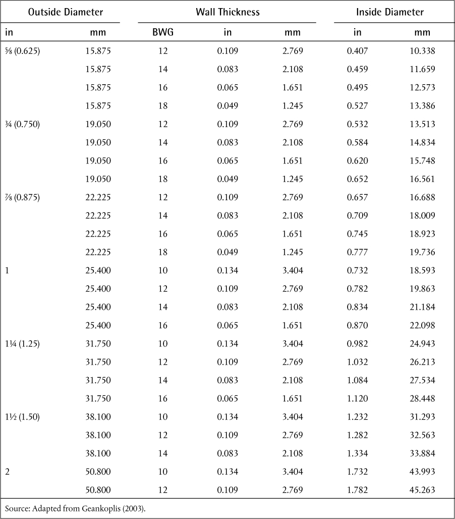
For S-T heat exchanges, the sizes of standard tubes are given in Table 2.4. The third column heading is BWG, which stands for Birmingham Wire Gauge, which is a standard method, albeit a very old standard, of specifying tube wall thickness. Unlike schedule pipe sizes discussed in Chapter 1, where the nominal pipe size does not correspond to any actual dimension of the pipe, the stated diameter of BWG tubing is the outside diameter. Standard tube sizes are virtually always used in heat-exchanger design, because the cost of customized tubes and the associated fittings and tooling would be prohibitively expensive. Standard lengths for tubes used in heat-exchanger design are from 8 ft to 20 ft (2.438–6.096 m) in 2 ft increments. The number of tubes that can fit in standard shell diameters is given in the tube-count tables shown later in Section 2.7.
2.5.3 Correlations for Film Heat Transfer Coefficients
The following sections cover the estimation of the convective film heat transfer coefficients. The cases for convective flow without phase change for inside and outside tubes (internal and external flows) are covered first. The coefficients for a change of phase are then introduced.
2.5.3.1 Flow Inside Tubes
In heat-exchanger design, the most common geometry for the equipment uses circular tubes, and the bulk of correlations and experimental work has been done for this geometry. The type of flow, turbulent, laminar, or transition, has a strong influence on the form of the correlation used to determine the film heat transfer coefficient. Each flow regime is considered separately in the following sections.
Turbulent Flow
For a fluid flowing inside a tube or pipe, the heat transfer coefficient is a function of fluid properties, fluid velocity, and the diameter of the tube. Many correlations exist for estimating the heat transfer coefficients for flow in tubes, and one of the most common is the Seider-Tate (1936) equation:

where Nu is the Nusselt number, Re is the Reynolds number, and Pr is the Prandtl number. The Prandtl number is the ratio of the rate of viscous diffusion to the rate of thermal diffusion. The Seider-Tate correlation, Equation (2.26), is valid for all fluids (except molten metals) for Re ≥ 6000. All the fluid properties (ρ, μ, cp, k) should be evaluated at the average bulk temperature with the exception of μw, which is evaluated at the average wall temperature. The first term in parentheses on the right-hand side takes account of the entrance effects for short tubes. For the case when L/D > 72, the error in neglecting this term is <5%. The last term in parentheses on the right-hand side takes account of the viscosity change near the tube wall that affects the thickness of the thermal boundary layer. Usually this term is close to unity, partly due to the small exponent. However, the term may become important for highly viscous fluids, where large changes in viscosity may take place because of the temperature variation between the bulk fluid and the wall. The heat transfer coefficient determined from Equation (2.26) changes along the length of the heat exchanger as the viscosity at the wall changes with temperature and position; therefore, use of the Seider-Tate equation with the viscosity correction requires an iterative procedure.
Another common correlation is the Dittus-Boelter (1930) equation that is given by
where the value of the exponent n is 0.3 when the fluid is being cooled and 0.4 when the fluid is being heated. This equation does not require an iterative solution but is generally less accurate than Equation (2.26), especially for fluids undergoing large temperature changes.
For an annulus, the following equation can be used:

where Di−o is the inside diameter of the outer pipe and Do−i is the outside diameter of the inside pipe, and DH is hydraulic diameter of the annular opening = (Di−o − Do−i), where DH is defined in Equation (2.29).
For noncircular ducts (square, rectangle, triangular, and ellipsoidal), Equations (2.26) and (2.27) can still be used except that the hydraulic diameter, DH, should be substituted for Di in the equation (and in the definition of Re), where

The use of Equations (2.26) and (2.27) is illustrated in Example 2.7.
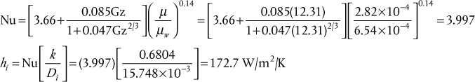
Use Equation (2.26) to determine the inside heat transfer coefficient for a fluid flowing inside a 12 ft (3.6576 m) long, ¾-in tube (16 BWG) at a velocity of 2 ft/s (0.6096 m/s) that is being cooled and has an average temperature of 212°F (100°C) and an average wall temperature of 104°F (40°C).
Consider the following three fluids:
a. Liquid water
b. n-cetane
c. Air at 2 atm pressure—use a velocity of 20 ft/s (6.609 m/s)
d. Compare the results using Equation (2.27).
Solution
From Table 2.4, Di = 0.620 in (15.748 mm)
a. For water at 100°C,
ρ = 961 kg/m3, μ = 0.000282 kg/m/s, cp = 4216 J/kg/K, k = 0.6804 W/m/K
At 40°C,
μ = 0.000654 kg/m/s
Applying Equation (2.26),

ρ = 717.6 kg/m3, μ = 0.0009207 kg/m/s, cp = 2392 J/kg/K, k = 0.1236 W/m/K
At 40°C,
μ = 0.002266 kg/m/s
Applying Equation (2.26),
hi = 534 W/m2/K (Re = 7482, Pr = 17.81)
c. For air at 2 atm pressure at 100°C,
ρ = 1.8907 kg/m3, μ = 2.183 × 10⁻⁵ kg/m/s, cp = 1008 J/kg/K, k = 0.0313 W/m/K,
At 40°C,
μ = 1.916 × 10⁻⁵ kg/m/s
Applying Equation (2.26),
hi = 57.9 W/m2/K (Re = 8315, Pr = 0.703)
d. Using the Dittus-Boelter equation, Equation (2.27) gives

Summarizing the results:
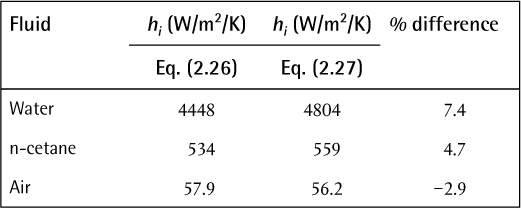
From the results of Example 2.7, three important points emerge. First, heat transfer coefficients for liquid water are generally significantly higher than for other liquids. Second, heat transfer coefficients for gases are normally much lower (~5–10 times) than for liquids. Third, while the Seider-Tate and Dittus-Boelter equations give different heat transfer coefficients, the differences are not that large and may be within typical design tolerances.
Transition Flow
For the transition between laminar and fully developed turbulent flow, the equation of Hausen (1943) satisfies both the upper and lower limits of Reynolds numbers and is recommended.

Laminar Flow
When the flow of fluid inside the tube is laminar (Re < 2100), then theoretical analyses for certain cases are possible and may be used to determine the heat transfer coefficient. Two limiting cases, constant heat flux at the wall and constant wall temperature, are normally considered. Neither case applies directly to normal operating conditions in process heat exchangers. However, the case for constant wall temperature is often used as a starting point for the development of suitable correlations. The appropriate equation to use is determined by the magnitude of the Graetz number, Gz, where ![]() . The correlations attributed to Hausen (1943),
. The correlations attributed to Hausen (1943),
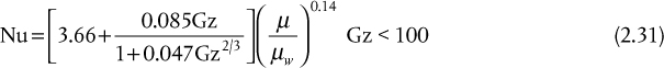
and Seider and Tate (1936),

are recommended.
It should be noted that Gz is a function of 1/L, so the heat transfer coefficient is strongly affected by the tube length. As the tube length becomes very long and Gz tends to zero, the Nusselt number tends to a limiting value of Nu∞. When viscosity corrections are negligible, it can be seen that Nu∞ = 3.66 assuming constant wall temperature.
Example 2.8 demonstrates the use of the equations for laminar flow.
Consider the same conditions and fluids in Example 2.7, except use a liquid velocity of 0.1 ft/s (0.03048 m/s) and a gas velocity of 2 ft/s (0.6096 m/s).
Solution
a. For water,
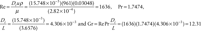
Applying Equation (2.31),
b. For n-cetane,
Re = 374.1, Pr = 17.8181, Di/L = 4.306 × 10⁻³, Gz = (374.1)(17.8181)(4.306 × 10⁻³) = 28.70, Nu = 4.719, hi = 37.04 W/m2/K
Re = 415.7, Pr = 0.7030, Di/L = 4.306 × 10⁻³, Gz = (415.7)(0.7030)(4.306 × 10⁻³) = 1.258, Nu = 3.831, hi = 7.61 W/m2/K
Summarizing the results:
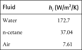
Clearly, the heat transfer coefficients for laminar flow are much lower than for turbulent flow. In general, laminar flow should be avoided except for highly viscous liquids where pumping costs needed to give turbulent flow conditions may become prohibitively large.
For laminar flow in annuli, the heat transfer correlation of Chen, Hawkins, and Solberg (1946) is recommended:

where Re and Gz are based on the hydraulic diameter, DH, μw is the viscosity at the inner wall of the annulus (at Do−i), and Di−o and Do−i are the inside diameter of the outside tube and the outside diameter of the inside tube, respectively.
For flow in rectangular channels, the limiting value of Nu for a constant wall temperature and very long channels (Nu∞) is a function of the ratio of the shorter to longer dimensions of the channel (0 < a/b < 1). The equivalent limiting value for tubes is 3.66, which is the first term on the right-hand side of Equation (2.31). The relationship between Nu∞ and (a/b) for rectangular channels attributed to Clark and Kays (1953) is shown in Figure 2.25 and Equation (2.34).
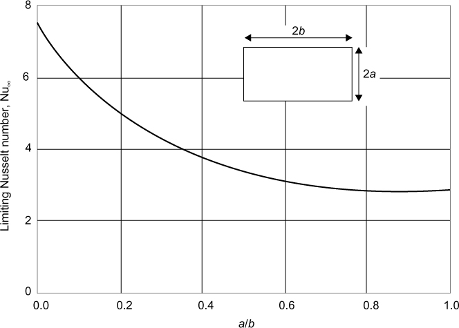
Figure 2.25 Relationship between Nu∞ and the ratio of the channel side lengths for rectangular channels (Clark and Kays [1953])

It is suggested that Equation (2.31) be modified to use with rectangular channels as

where Nu∞ is taken from Equation (2.34) and the hydraulic diameter is used in determining Re in Gz.
2.5.3.2 Flow Outside of Tubes (Shell-Side Flow)
The estimation of the heat transfer coefficient for the flow of a fluid over a bundle of tubes is very complicated. Referring back to Figure 2.18, in an S-T exchanger, the flow on the shell side is parallel with the tube axis for some portion of the flow path and perpendicular to the tube axis for the remainder of the time. Moreover, the flow path of the shell-side fluid is quite tortuous, since it flows around and between the tubes, and the arrangement of the tubes (square or triangular pitch) significantly affects the mixing and turbulence of the fluid. Needless to say, analytical expressions for heat transfer coefficients do not exist, and the number of correlations for overall shell-side heat transfer coefficient are numerous. In this section, some of the different phenomena occurring on the shell side of the heat exchanger are discussed, and a simplified method for calculating shell-side coefficients is presented.
Flow Normal to the Outside of a Single Cylinder
The flow of fluid normal to a single tube or cylinder is a complex but well-studied process. A review of data over a wide range of fluid properties (Pr) and flow conditions (Re) has been performed by Žukauskas (1972) and Churchill and Bernstein (1977). The equation recommended by Žukauskas is

where subscripts w, f, and bulk refer to the wall, film, and bulk fluid conditions, respectively.  is evaluated using the fluid approach velocity upstream of the tube, and the film properties are evaluated at the average film temperature, Tf = (Tbulk + Tw)/2. Finally, the different Prandtl numbers in Equation (2.36) are evaluated at the average film temperature, wall temperature, or bulk fluid temperature depending on the subscript.
Equation (2.36) is valid for values of Pr in the range 0.7 to 500. The values of C and m depend on the Reynolds number and are given in Table 2.5.
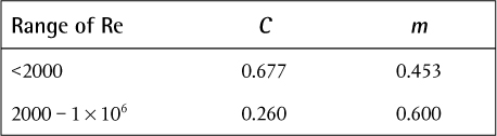
Table 2.5 Values for Parameters in Equation (2.36)
Flow Normal to Banks of Tubes
The heat transfer coefficient for a fluid flowing normal to a bank of tubes is very complicated, and the average coefficient for a given tube will vary depending on the location of the tube in the bank. A good review of data on tube banks is again given by Žukauskas (1972). In this chapter, a simpler method for estimating an average shell-side heat transfer coefficient attributed to Kern (1950) is presented.
Kern’s Method for Shell-Side Heat Transfer
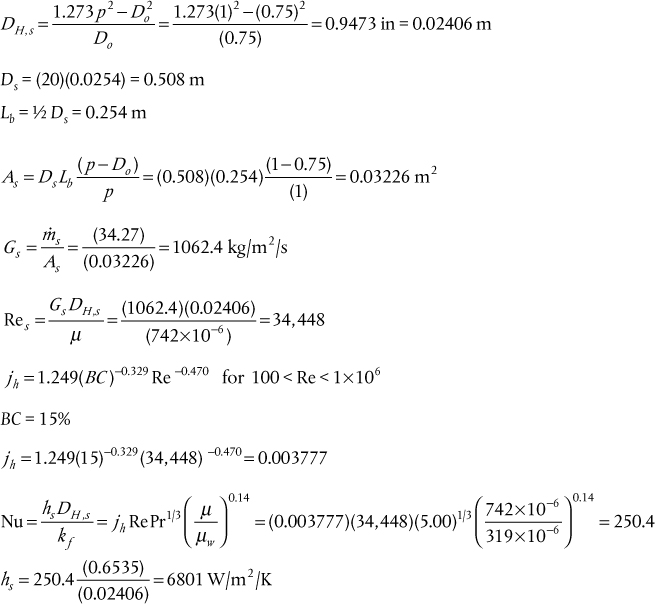
A popular method for making a preliminary estimate of the shell-side heat transfer coefficient and shell-side pressure drop is that attributed to Kern (1950). The correlations used in Kern’s method depend on an equivalent hydraulic diameter for the shell side, DH,s. Figure 2.26 shows the basic tube arrangements, and equations for the hydraulic diameter are
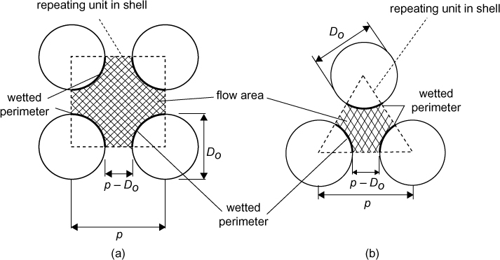
Figure 2.26 Notation for determining the hydraulic diameter of shell-side flow: (a) square pitch, (b) triangular pitch
Square pitch

Triangular pitch

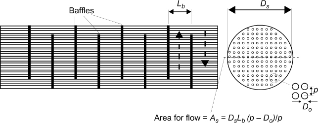
The term (p − Do) is sometimes referred to as the clearance, C. The shell-side fluid changes velocity as it passes through the baffle window and travels across the bank of tubes. This situation is illustrated in Figure 2.27, where the inside diameter of the shell is Ds, and the baffle spacing is Lb.
Assuming that the mass flowrate of fluid on the shell side is ![]() , then using the notation in Figures 2.26 and 2.27, the following parameters are defined:
, then using the notation in Figures 2.26 and 2.27, the following parameters are defined:
Shell-side superficial mass velocity,

Shell-side velocity,
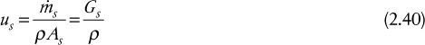
where the As is the maximum flow area on the shell side given as
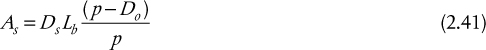
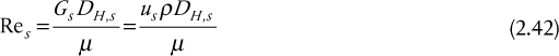
Shell-side Reynolds number,
The average heat transfer coefficient for the shell side of the exchanger is given by
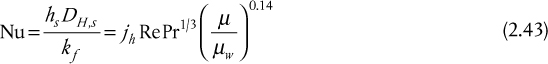
where
where BC is the baffle cut as a percentage of the shell diameter, with typical values from 20% to 35%.
The frictional pressure drop through the shell side of the exchanger is then given by
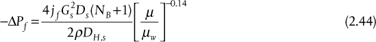
where
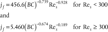
It should be noted that the original method attributed to Kern (1950) uses a series of charts to determine the values of jh and jf as functions of Re and BC. However, the equations given for jh and jf were found by regressing data from these charts and are accurate enough for preliminary designs.
Example 2.9 illustrates the use of Kern’s method for estimating the heat transfer coefficient for a bank of tubes. This method will also be used to design a heat exchanger in Section 2.7.
Water flows across the outside of a bank of tubes. It enters at 30°C and leaves at 40°C. The water enters at a flowrate of 34.27 kg/s, the shell diameter is 20 in, the baffle spacing is half (¼) the shell diameter, the baffle cut (BC) is 15%, and ¾-in outside diameter (OD) tubes on a 1-in pitch are used. The fluid inside the tubes may be assumed to be at a constant temperature of 90°C (condensing organic), the inside coefficient is expected to be much higher than the shell-side coefficient, and thus the wall temperature may be taken as 90°C.
Use Kern’s method to determine the average heat transfer coefficient for the shell side for the following arrangements:
a. Square pitch
b. Equilateral triangular pitch
Solution
a. Tubes on a square pitch

From Equations (2.37), (2.41), (2.42), and (2.43),
b. Tubes on a triangular pitch
From Equations (2.38), (2.41), (2.42), and (2.43),

Assume a 15% baffle cut:
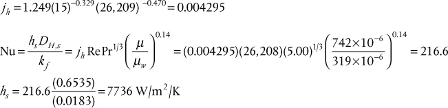
It can be seen that a higher heat transfer coefficient is obtained using triangular pitch. However, this will usually come at the expense of a higher shell-side pressure drop.
2.5.3.3 Boiling Heat Transfer
When one or both fluids undergo a change in phase, the heat transfer process is much more complex and, in general, will be less influenced by the rate of flow of material past the heat transfer surface than by the temperature driving force between the surface and the bulk fluid temperature. There is a large body of work in the area of boiling heat transfer that is far too extensive to review here. The approach adopted in this text is to provide a brief overview of boiling phenomena and to present some useful working equations that are applicable to the design of process heat exchangers.
Typical Pool Boiling Curve
A typical boiling curve for water at 1 atm pressure is shown in Figure 2.28 and represents the situation when a heated surface is placed in a pool of water. In the figure, the x-axis represents the temperature difference between the heating surface (Ts) and the saturation temperature (Tsat), and the y-axis is the heat flux (Q/A). The behavior of water at other pressures and other liquids below the critical pressure mimics the general trends shown in Figure 2.28.

When the temperature difference between the surface and saturation temperatures of the water (Tsat =100°C for water at 1 atm) is less than 5°C, all vapor is produced by evaporation at the liquid surface, and the process is termed free convection boiling. In this region, the heat transfer coefficient is proportional to (ΔTs)¼. As ΔTs increases beyond about 5°C, bubbles of vapor appear on the heating surface, detach, and move to the surface of the liquid. At first, bubbles appear at certain preferred nucleation sites on the surface, but as the ΔTs increases, the number of nucleation sites increases, and more bubbles are produced. The bubble motion near the surface tends to increase turbulence and promotes higher heat transfer. This process is known as nucleate boiling. In this boiling regime (region a–c), the heat transfer coefficient is a strong function of ΔTs and h ∝ (ΔTs)n where n is between 2 and 3. As ΔTs increases further, more and more bubbles are formed at the surface, and they start to interfere with the movement of liquid toward the surface. This phenomenon tends to reduce the heat transfer coefficient because the gas has a much lower heat capacity and thermal conductivity than the liquid. As a result, an inflection point (Point b) is seen in the boiling curve (at 10°C). With further increase in ΔTs, the increase in the rate of bubble formation eventually causes the heat flux to reach a maximum (at about 30°C). At Point c on Figure 2.28, the path by which the process proceeds to the right depends on how the experiment is conducted.
First, consider the case when the temperature of the heat transfer surface can be increased independently of the heat flux. Increasing ΔTs beyond Point c is accompanied by a reduction in heat transfer coefficient (and heat flux) due to the intermittent formation of a vapor film at the heat transfer surface, which occurs because the rate of bubble formation is faster than the rate of bubble detachment from the surface. This region is termed the partial film boiling regime (Region c–d), and the heat transfer surface may at any time be completely covered by either gas or a liquid-bubble mixture. In this regime, the surface oscillates between a nucleate boiling and a film boiling condition. This behavior leads to a reduction in heat flux and a corresponding reduction in heat transfer coefficient. This behavior persists until ΔTs is large enough to maintain a stable gas film at the surface, and then the film boiling regime is reached (Region d–e). The transition to the film boiling regime occurs at the point of minimum heat flux, Point d, which is referred to as the Leidenfrost point. As ΔTs increases beyond the Leidenfrost point, the heat transfer coefficient and heat flux increase because of a combined effect of increasing gas thermal conductivity with increasing temperature and radiation heat transfer that is present at the high temperatures required for film boiling.
Consider now the case when the experiment is conducted with the heat flux as the controlled or independent variable and ΔTs is the dependent variable, which would be the case if, for example, an electric heater or a direct flame was used to heat the surface in contact with the liquid. Using this experimental procedure, the boiling curve would be identical to that described previously from Points a to c, but at Point c, the only way that the heat flux can be increased is for ΔTs to jump to Point e. This would be accompanied by a very large increase in Ts, which may lead to permanent damage to the heated surface or in extreme cases could melt the surface.
It is important to recognize that this temperature jump at the critical heat flux may occur in actual processes in which the energy for boiling is supplied by an electric heater or by a burning fuel, as would be the case in a gas or oil fired heater or boiler. This phenomenon generally cannot happen if heat is supplied by a hot process stream, because the temperature of the process stream is bounded by process conditions and the heat flux is, therefore, also bounded. As a result, process heat exchangers used for raising steam such as waste heat boilers or used for reboiling a distillation column do not exhibit this unstable behavior. Nevertheless, operation to the right of the critical heat flux is generally avoided in process heat exchangers to avoid the effect that as ΔT increases the heat flux decreases. Such inverse and counterintuitive behavior may cause problems with control and diagnosis of operations. For process heat exchangers, operation in the nucleate boiling regime is recommended.
Determining the Critical or Maximum Heat Flux in Pool Boiling
Many equations exist to predict the maximum heat flux, denoted by Point c in Figure 2.28. A recommended correlation that gives good predictions is that attributed to Zuber (1958):
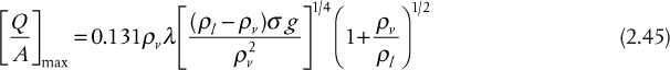
where ρl and ρv are the densities of saturated liquid and vapor, respectively, λ is the latent heat of vaporization, and σ is the surface tension of the boiling liquid.
An alternative relationship that requires only the critical pressure is given by the Cichelli-Bonilla (1945) correlation:
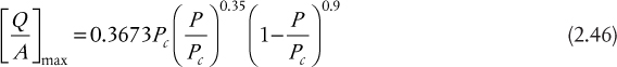
where [Q/A]max is given in W/m2 and pressure is in Pa.
Estimate the critical heat flux for water at 1 atm pressure using Equations (2.45) and (2.46) and compare with the value given in Figure 2.28.
Properties of water at 1 atm pressure (P = 1.013 × 10⁵ Pa) and T = 100°C ρl = 958 kg/m3, ρv = 0.598 kg/m3, λ = 2.257 × 10⁶ J/kg, σ = 0.060 N/m, Pc = 22.06 × 10⁶ Pa
Solution
From Equation (2.45),
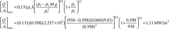
From Equation (2.46),

From Figure 2.28, ![]()
Thus both predictions are within ±10%.
Heat Transfer Coefficient for Nucleate (Pool) Boiling
Perhaps the most widely used correlation for the nucleate pool boiling regime is that attributed to Rohsenow (1964)

where l and v refer to saturated liquid and vapor conditions, s = 1.0 for water and 1.7 for other materials, and Cf is a constant that depends on the material of the heated surface and varies between 0.006 and 0.013.
This gives the equivalent heat transfer coefficient as
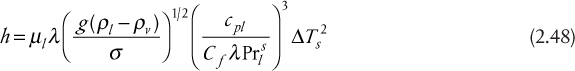
The application of Equations (2.47) and (2.48) is illustrated in Example 2.11.
Use Equations (2.47) and (2.48) to estimate the heat flux and heat transfer coefficient for water at 1 atm pressure for a temperature driving force of 10°C.
Solution
Properties of water at 1 atm pressure (P = 1.013 × 10⁵ Pa) and T = 100°C ρl = 958 kg/m3, ρv = 0.598 kg/m3, λ = 2.257 × 10⁶ J/kg, σ = 0.060 N/m, cpl = 4216 J/kg/K, μl = 2.82 × 10⁻⁴
![]()
Applying Equation (2.47) with s = 1.0 and Cf = 0.013 gives
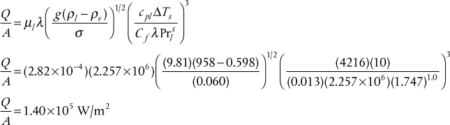
The equivalent heat transfer coefficient, from Equation (2.48), is h = 14,000 W/m2/K.
From Figure 2.28, the value of the heat flux for ΔT = 10°C (Point b) is approximately 1.5 × 10⁵ W/m, or about 10% higher than the predicted value. It should be noted that the factor Cf was chosen as 0.013, which is a conservative estimate. The value of Cf has a very strong influence on the flux, and generally Cf may not be known for practical situations. The resulting heat transfer coefficient is very high, even using this value of Cf. In practice, the heat transfer coefficient for boiling is hardly ever the limiting heat transfer coefficient, and hence using a conservative value of Cf will not lead to significant errors in estimating the overall heat transfer coefficient U.
Effects of Forced Convection on Boiling
The conditions for pool boiling described in the previous sections are generally not those present in process heat exchangers, with the exception of a kettle-type reboiler, in which a vapor is generated in the shell side of the heat exchanger. Often, boiling is accompanied by a significant bulk flow of fluid. For example, if liquid is pumped through vertical (or horizontal) tubes that are surrounded by fluid (on the shell side) that is hot enough to boil the liquid in the tubes, then the heat transfer process becomes much more complicated. The processes occurring for this situation are illustrated in Figure 2.29.
For the flow in a vertical tube, from Figure 2.29(a), it can be seen that boiling starts at the bottom of the tube at some point above the inlet and results in a bubbly flow. As bubbles start to coalesce and form bigger spherical-cap-shaped bubbles, the flow pattern becomes more chaotic, and large slugs start to form and move rapidly upward. As more of the liquid becomes vaporized, there is a transition region where the continuous phase switches from liquid to vapor. The liquid tends to move up the tube at the walls, and the vapor forms a core at the center of the tube, in which nonvaporized liquid drops travel. Above the core-annular region, all the liquid at the walls has been vaporized, and the entrained drops of liquid in the vapor rapidly evaporate until only vapor exists. If the tube extends further vertically, then superheating of the vapor will occur. The situation for forced boiling in horizontal tubes is illustrated in Figure 2.29(b). The flow pattern in the horizontal flow mimics the vertical flow pattern in many ways. The big difference between the two orientations is that for horizontal flow, gravity tends to force the liquid to the bottom of the tube and the flow pattern is not radially symmetrical, as shown by the inserts above the figure. It should also be apparent that the local heat transfer coefficient varies widely over the range of conditions in the tube, which is also shown in Figure 2.29(b).
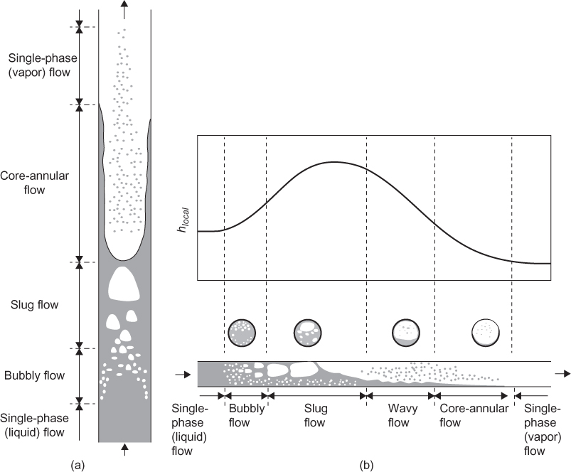
Figure 2.29 Heat transfer processes and flow regimes occurring when fluid is pumped through a tube and vaporizes: (a) vertical tube, (b) horizontal tube
From the description of the flows given for these two orientations, it is clear that the heat transfer coefficient probably changes significantly over the length of the tube. Moreover, the flow patterns are very complex and depend on many parameters. Indeed, the accurate prediction of pressure drop for these two-phase flows is difficult. There have been many attempts to correlate heat transfer coefficients with the flow regimes and also in combination with parameters that describe the two-phase pressure drop. The approach used here is to give the results from a study by Gungor and Winterton (1986), in which correlations were developed for a large set of data taken from a wide variety of boiling liquids in horizontal and vertical tubes. The authors claim that the correlation is able to predict the data within ±25%. The general form of their correlation is
where hcb is the overall convective boiling coefficient, hl is the convective coefficient for liquid flow in the tube, and hpb is the pool boiling coefficient. The factor f, which is greater than 1, accounts for the much higher velocities for two-phase flow compared with single-phase flow. This factor was correlated against the two-phase Martinelli parameter, Xtp, and is given by

where Xtp is the Martinelli two-phase flow parameter given by

where x is the stream quality (mass fraction of vapor in the stream), and density and viscosity are for the saturated liquid and vapor conditions. Bo is a boiling number and is given by
where Q/A is the heat flux, λ is the latent heat of vaporizations, and G is the superficial mass velocity flowing (axially) past the heating surface. In using Equations (2.51) and (2.52), it should be noted that as x → 0 or 1, the equations are no longer valid. These limits, however, are represented by the pure convective heat transfer coefficients for all liquid flow and all vapor flow, respectively.
The parameter s in Equation (2.49) is a “suppression” factor that is less than 1 and accounts for the lower superheat that is available in convective boiling compared to pool boiling alone. This parameter is given by

where Rel is the Reynolds number for the flow inside the tube assuming that the flow is all liquid.
The convective coefficient in Equation (2.49), hl, is taken to be from the Seider-Tate or Dittus-Boelter correlations (Equation [2.26] or [2.27]) for the liquid. The recommended expression for pool boiling is taken from the correlation attributed to Cooper (1984) and is given by
or
where Pr is the reduced pressure, M is the molecular weight (g/mol) and (Q/A) is the heat flux (W/m2), and the units of hpb are W/m2/K. The pool boiling coefficient from Equation (2.48) could alternatively be used instead of Equation (2.54).
The sequence of Equations (2.49) to (2.54) must be solved to determine the convective boiling heat transfer coefficient and in general will require an iterative method because the heat flux (Q/A) is imbedded in the boiling number term Bo (and Equation [2.52]), which will not be known a priori. Moreover, the value of hcb changes along the length of the tube as the vapor quality changes. An illustration of the use of equations for forced convection boiling is given in Example 2.12.
An organic liquid (1-propanol at 1 bar) is to be vaporized inside a set of vertical 1-in BWG 16 tubes using condensing steam on the outside of the tubes to provide the energy for vaporization. The major resistance to heat transfer is expected to be on the inside of the tubes, and the wall temperature, as a first approximation, may be assumed to be at the temperature of the condensing steam, which for this case is 110°C. It may be assumed that the value of the vapor quality, x, varies from 0.01 to 0.99 in the tube. The flow and other physical parameters for the organic liquid are
ρv = 2.003 kg/m3, ρl = 732.5 kg/m3, μv = 9.617 × 10⁻⁶ kg/m/s, μl =455.8 × 10⁻⁶ kg/m/s, Tsat = 96.9°C, Pc = 52 bar, M = 60 g/mol, kl = 0.1406 W/m/K, λ = 693.5 kJ/kg, cp,l = 3215.1 J/kg/K, ![]() = 0.04 kg/s/tube, Di = 0.745 in = 18.923 × 10⁻³ m
= 0.04 kg/s/tube, Di = 0.745 in = 18.923 × 10⁻³ m

Determine the average heat transfer coefficient and the length of the tube needed to vaporize the liquid in this vertical reboiler.
Solution
From Equation (2.55), the pool boiling coefficient is given by

The convective heat transfer coefficient is given by Equation (2.26), assuming that L >> D and μw ≅ μ1, then

From Equation (2.51),

The value of x in the preceding equation varies from 0.01 to 0.99, and hence Xtp will also vary over a wide range. To account for the change in x, the problem will be discretized with respect to x and solved for each increment of Δx = 0.1. The calculations for x = 0.01 to 0.1 will be covered, and then the results for the other increments will be summarized. To calculate f in Equation (2.50), the value of Bo must be found from Equation (2.52); however, the heat flux (Q/A) is unknown. Using the discretization scheme shown in Figure E2.12A, the value of B0 may be found in terms of the tube length Δzi.
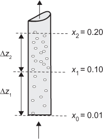
Figure E2.12A Discretization scheme used in Example 2.12
Therefore, for the first increment is

In the equation for Bo, the amount of heat required to vaporize the stream from a vapor fraction of xo to x1 is simply ![]() (x1 − xo)λ, and the surface area of the tube required for this to happen is πDiDz1. By guessing a value for Δz1, the values of f and s from Equations (2.50) and (2.53) can be calculated and used in Equation (2.49) to calculate hcb. Now an energy balance on the first increment of tube gives
(x1 − xo)λ, and the surface area of the tube required for this to happen is πDiDz1. By guessing a value for Δz1, the values of f and s from Equations (2.50) and (2.53) can be calculated and used in Equation (2.49) to calculate hcb. Now an energy balance on the first increment of tube gives
and rearranging
The solution for the first increment is found by iterating between Equations (2.49) and (E2.12) until a constant value of Δz1 is obtained.
For the first iteration, choose a value of Δz1 = 0.5 m:
and

Substitute into Equation (E.2.12) to get
Now recalculate B0 and iterate until to Δz1 does not change; finally this gives Δz1 = 0.635 m. The results for the whole range of x from 0.01 to 0.99 are given in Table E2.12.
Therefore, a tube length of 3.488 m (11.4 ft) is required. The average heat transfer coefficient for this service is found from
From Equation (2.46), the maximum heat flux for pool boiling is given by

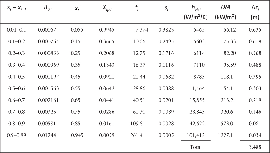
Table E2.12 Results for Convective Boiling Heat Transfer as a Function of Distance from the Entrance
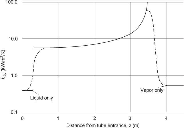
The critical heat flux of 471 kW/m2 is exceeded at the end of the tube (x > 0.9), but this critical value is for quiescent pool boiling, and the effect of convection means that flux values above the critical value are possible. Alternatively, the flux could be limited to the value of 471 kW/m2 but the effect on the required tube length would be very small. Therefore, the estimate of a 3.49 long tube is reasonable.
One last point of interest is the relationship between hcb and distance from the entrance given in Table E2.12, which is shown in Figure E2.12B.
The basic shape of the curve appears to be somewhat different from that given in Figure 2.29. However, as noted previously, for x = 0 the liquid convective coefficient should be used, and for x =1 the gas convective coefficient should be used, and these limits are shown on the figure. The transition from the convective boiling correlation of Gungor and Winterton (1986) to these single-phase limits is not predicted, but the general trend in the results from this example do follow the shape of Figure 2.29, and a dashed curve showing possible transitions from the single- to two-phase regimes is shown in Figure E2.12B.
Film Boiling
When the temperature driving force between the tube wall and the boiling liquid exceeds a critical value (Point d, the Leidenfrost point on Figure 2.28), then the heat transfer enters the film boiling regime. This regime is characterized by a coherent continuous film of vapor covering the heat transfer surface. The recommended correlation for the film boiling regime on the outside of a horizontal tube is attributed to Bromley (1950):

where the bar over the symbol represents an average heat transfer coefficient over the length of the tube. Often, the convective heat transfer coefficient in Equation (2.56) is augmented by a radiation component that becomes increasingly important as the absolute temperature difference between the surface and the boiling point of the liquid increases. When this is the case, the overall heat transfer coefficient, ![]() , should be calculated from
, should be calculated from
where ![]() is calculated from
is calculated from

where ɛ is the emissivity of the tube surface, σ is the Stefan-Boltzmann constant (5.6704 × 10⁻⁸ W/m−2/K−4), and the temperatures used in Equation (2.58) are absolute (Kelvin). It should be clear that when radiation is important, the calculation of the boiling film heat transfer coefficient using Equations (2.56), (2.57), and (2.58) is an iterative process.
Calculate the heat transfer coefficient for water boiling at 42 bar pressure (253.3°C) in the shell side of a waste heat boiler equipped with 1.25 BWG 12 tubes.
Assume that the tube wall temperature is constant at 400°C, and include radiation from the wall that has an emissivity of 0.40.
Solution
ρv = 21.14 kg/m3, ρl = 732.5 kg/m3, μv = 19.11 × 10⁻⁶ kg/m/s, Tsat = 253.3°C, MW = 18, kv = 0.0442 W/m/K, λ = 1697.8 kJ/kg, D = 1.25 in = 0.03175 m
From Equation (2.56),
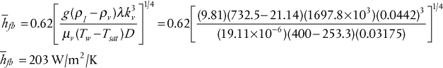
From Equation (2.58),
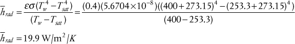
From Equation (2.57),
Solving gives
This represents a 7% increase in hfb due to radiation effects.
2.5.3.4 Condensing Heat Transfer
If a vapor is exposed to a cold surface and the liquid does not wet the surface, then the vapor will condense by forming small drops or beads of liquid on the surface. This phenomenon is sometimes seen on window panes and car windshields, when the outside temperature drops and water from the warm humid air inside starts to condense on the cold glass. This phenomenon is known as dropwise condensation. The beads that form roll off the surface if it is inclined to the vertical or form a pool on a horizontal surface. Dropwise condensation does not occur, except in rare circumstances, in process heat exchangers, because the surfaces are not smooth and clean but are rough due to fouling and surface scaling. For most practical circumstances, vapors condense on heat-exchanger surfaces by a film condensation mechanism discussed next.
When a vapor close to its saturation temperature, Tsat, is exposed to a cold surface at a temperature below Tsat, then condensation of the vapor occurs on the surface.
In heat exchangers, this process is often accomplished by exposing a saturated vapor on the shell side of an S-T exchanger to horizontal (or vertical) tubes through which a cooling liquid is passed. At steady state, the liquid forms a film around the circumference of the tube and falls by gravity onto tubes situated below it. This phenomenon is illustrated in Figure 2.30(a).
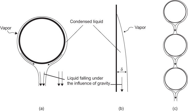
Figure 2.30 Liquid condensing on a cold surface: (a) horizontal tube, (b) vertical plate, and (c) a bank of multiple horizontal tubes
Shown in Figure 2.30(b) is the condensation of liquid on a flat, vertical plate. As the liquid falls, the liquid layer increases in thickness, and the resistance to heat transfer increases because the path for energy flow through the liquid film becomes longer. In Figure 2.30(c) the condensation on a stack of vertically aligned horizontal tubes is illustrated.
Nusselt’s Analysis of Falling-Film Condensation
Using the following assumptions regarding the flow of condensate on a vertical flat plate, Nusselt analyzed the heat transfer process that occurs across the film of flowing liquid condensate:
• Laminar flow of fluid with constant physical properties
• Gas is a pure vapor at Tsat. Condensation occurs only at the vapor-liquid interface, that is, no heat transfer resistance in gas
• Shear stress at the liquid-vapor boundary is zero, that is, no vapor velocity or vapor thermal boundary layer effects
• Heat transfer across the liquid film is only by conduction
Nusselt’s analysis leads to the following expression for the average heat transfer coefficient over the length, L, of the plate:
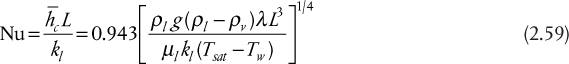
Alternatively, the average heat transfer coefficient can be written as
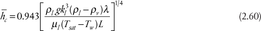
where, according to McAdams (1954), all the physical properties of the liquid should be evaluated at the average film temperature, Tf = Tsat − 0.75(Tsat − Tw).
The total rate at which liquid condenses can then be determined via an energy balance as

The condition for which the expression in Equation (2.60) is valid is determined on the basis of the value of an effective Reynolds number for the falling film, Reδ, given by
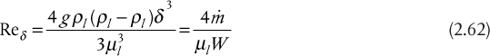
where δ is the thickness of the falling film (Figure 2.30[b]) and ![]() is the mass flow rate of condensate falling down a plate of width W. Equation (2.60) is valid for Reδ ≤ 30. For the region 30 ≤ Reδ ≤ 1800, the flow down the plate is described as wavy laminar and there is a slight enhancement of the heat transfer coefficient such that
is the mass flow rate of condensate falling down a plate of width W. Equation (2.60) is valid for Reδ ≤ 30. For the region 30 ≤ Reδ ≤ 1800, the flow down the plate is described as wavy laminar and there is a slight enhancement of the heat transfer coefficient such that ![]() from Equation (2.60) should be multiplied by E, where E is given by
from Equation (2.60) should be multiplied by E, where E is given by
Falling-Film Condensation on Cylinders
The result from Nusselt for laminar flow on a vertical flat plate is essentially correct, even for vertically oriented tubes, except the results from experiments suggest that the coefficient should be increased:
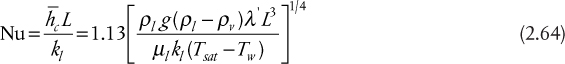
where the latent heat is modified to include subcooling in the film as
For the case when the flow in the film is turbulent (and Reδ,max > 1800), McAdams [1954] suggests the use of the following equation:
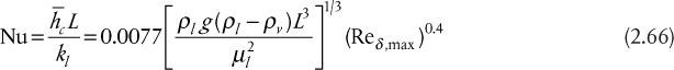
For film condensation on the outside of horizontally oriented tubes, the following expression was obtained by Nusselt:
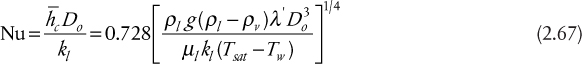
Because the path length for the film formation (~πDo/2) on tubes used for commercial heat exchangers is relatively small, turbulent flow rarely occurs in horizontal-tube condensers. An example to illustrate use of the correlations for condensing heat transfer is given in Example 2.14.
Example 2.14 (adapted from Bennett and Myers [1982], Problem 25.1)
An S-T condenser contains four rows of four copper tubes per row on a square pitch. The tubes are 1-in, 16 BWG and 6 ft long. Cooling water flows through the tubes such that hi = 1000 BTU/hr/ft2/°F. The water flow is high so that the temperature on the tube side may be assumed to be constant at 90°F. Pure saturated steam at 5 psig is condensing on the shell side. Determine the capacity of the condenser (Q in BTU/hr) if the condenser tubes are oriented (a) vertically, and (b) horizontally. You should assume that neither water nor steam fouls the heat-exchange surfaces.
Solution
The correct film temperature is unknown and depends on ho. The solution algorithm is
1. Guess ho
2. Calculate film temperature and film properties
3. Apply equation for ho and iterate
Guess ho = 1000 BTU/hr/ft2/°F
a. Vertical arrangement
Steam at 227°F, Do = 1.0 in = 0.0833 ft, Di = 0.87 in = 0.0725 ft, kcopper = 220 BTU/hr/ft/°F From Equation (2.23) (with no fouling coefficients for either stream),

For water at 179.8°F → k1 = 0.3882 BTU/h/ft/°F, ρ1 = 60.55 lb/ft3, λ = 960 BTU/lb (at 5 psig), μl = 0.8161 lb/ft/h, cp,l = 0.9720 BTU/lb/°F, ρv = 0.049 lb/ft3
Substituting values into Equation (2.64),

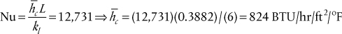
Iterating to find the new Tw and Tf gives
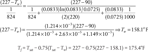
For water at 175.4°F → kl = 0.3873 BTU/h/ft/°F, ρl = 60.65 lb/ft3, λ = 960 BTU/lb (at 5 psig), μl = 0.8405 lb/ft/h, cp,l = 0.9718 BTU/lb/°F, ρv = 0.049 lb/ft3

One more iteration yields ![]() , which is close enough to the previous iteration:
, which is close enough to the previous iteration:
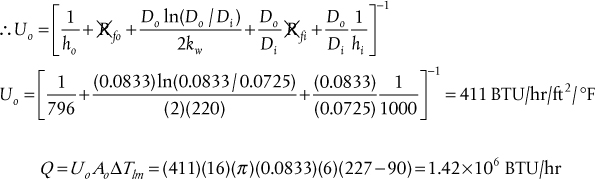
Check for Reδ:
Rδ < 1800, so the correct equation was used.
b. Horizontal arrangement
Use the same approach as used for vertical tubes.
For iteration 1, use the same temperatures and properties as for vertical tubes (Equation [2.67]):

Iterating to find the new Tw and Tf gives

For water at 190.5°F → kl = 0.3903 BTU/hr/ft/°F, ρl = 60.295 lb/ft3, λ = 960 BTU/lb (at 5 psig), μl = 0.7597 lb/ft/h, cp,l = 0.9728 BTU/lb/°F, ρv = 0.049 lb/ft3
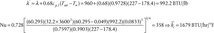
The third iteration gives ![]() , TW = 180.9°F, and Tf = 192.4°F.
, TW = 180.9°F, and Tf = 192.4°F.
The fourth iteration gives ![]() —this is close enough to the previous iteration.
—this is close enough to the previous iteration.

Check for Reδ:

The correct equation was used.
2.6 Extended Surfaces
From Examples 2.7 and 2.8, it is clear that the heat transfer coefficients for gases are generally much lower than for liquids or for phase changes. Indeed, the limiting heat transfer coefficient will be the gas film coefficient if a gas is one of the fluids in the exchanger. To increase the effective gas film coefficient, it is often necessary to add some form of extended heat transfer surface or fins to the gas side of the heat exchanger. Some examples of finned tubes were given in Figures 2.22 and 2.23. Some additional arrangements of fins are given in Figure 2.31.
From Figure 2.31, it can be seen that a wide variety of fin geometries is possible, and the equations describing the temperature profile in the fin can be quite complicated. In subsequent sections, the equations for both simple and more complicated geometries are presented without derivation.

Figure 2.31 Various fin types: (a) straight fin constant thickness, (b) spine or pin fin constant thickness, (c) annular fin constant thickness, (d) straight fin nonuniform thickness, (e) spine or pin fin nonuniform thickness, (f) annular fin nonuniform thickness, (g) longitudinal fin constant thickness
2.6.1 Rectangular Fin with Constant Thickness
A rectangular fin is shown in Figure 2.31(a). The equations describing the heat conduction in this type of fin, with a constant cross section, are formulated and solved in Appendix 2.B. A key parameter in analyzing the performance of a fin is the fin effectiveness defined as

For the rectangular fin, L is the length of the fin and δ is the thickness of the fin; the fin effectiveness is given by Equation (2.68) and is plotted in Figure 2.32. The term m is a dimensionless parameter that is defined in Equation (2.69).
The value of ɛfin indicates the efficiency by which the additional fin surface area is being utilized. For example, if the thermal conductivity of the fin material is very high or the fin is short, then, all else being equal, the temperature everywhere along the length of the fin is close to the wall temperature, and temperature driving force between the fin and the surroundings will be close to T0 − Tfluid. Therefore, the fin surface area is used effectively. If, on the other hand, the fin length, L, is very long compared with its thickness, δ, then the temperature of the fin over a major portion of its length is close to Tfluid, and the efficiency of the fin is low, since only a small portion of the fin (close to the wall) has a significant temperature driving force to exchange heat with the surrounding fluid. In other words, the good news is that the fin provides more area for heat transfer, but the bad news is that the driving force may decrease down the length of the fin, so all of the benefit of the increased area is not seen. The effectiveness factor quantifies this situation.

In the previous analysis, it was assumed that the tip of the fin did not lose any heat or that an adiabatic boundary condition at the end of the fin was used. This assumption is strictly correct only for fins with a very large value of L/δ. However, the results given in Equation (2.68) and Figure 2.32 can be used with great accuracy if a corrected fin length, Lc, is used, where
2.6.2 Fin Efficiency for Other Fin Geometries
2.6.2.1 Annular or Circular Fins of Uniform Thickness
These fins are shown in Figure 2.31(c), and the fin efficiency is given by

where  and Ii and Ki are modified Bessel functions of the first and second kind
of order i, respectively. Equation (2.71) is plotted in Figure 2.33.
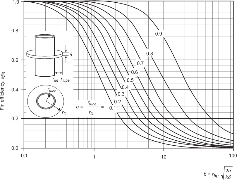
2.6.2.2 Narrow Triangular Fin
The efficiency for these fins, Figure 2.31(d), is given by

where  , and Equation (2.72) is plotted in Figure 2.34.
2.6.3 Total Heat Transfer Surface Effectiveness
Up until this point, the efficiency of single fins of different geometries has been considered. However, multiple fins are always used in real heat exchangers. Consider a set of fins stacked as shown in Figure 2.35. For the case of rectangular straight fins, shown in Figure 2.35(a), consider a section of wall of area W(δ + b). Without fins, this would be the area exposed to the fluid; with fins, the heat transfer area becomes Wb + 2LW. Assuming that the film heat transfer coefficient, h, between the surface and the surrounding fluid does not vary with position, then an energy balance for the surface gives
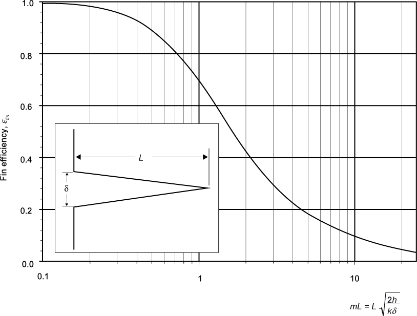
If Abase is the area of the surface not taken up by fins (equal to Wb for the section of wall considered) and Abare is the total surface area without fins (equal to W × (δ + b) for this example) and Afin is the area of the fins (equal to 2WL for the single fin considered in this example), then the results from Equation (2.73) can be generalized as follows:
With fins
Without fins
The enhancement in heat transfer is found by comparing Equations (2.74) and (2.75):

This enhancement of heat transfer depends on the geometry of the fins and the fin efficiency and is illustrated in Example 2.15.

Figure 2.35 Stacked arrangement of fins: (a) straight rectangular fins, (b) straight triangular fins, (c) straight annular fins.
An aluminum heat transfer surface that is maintained at 100°C is in contact with air at 20°C. The film heat transfer coefficient between the surface and the air is estimated to be 42 W/m2/K. Determine the area of bare surface equivalent required to transfer 4 kW of power and the enhancement in heat transfer for the following cases:
a. A bare flat metal surface
b. A flat metal surface equipped with 50 mm long, 3 mm wide rectangular aluminum fins placed on 10 mm centers
c. A flat metal surface equipped with 50 mm long, 3 mm wide-base triangular aluminum fins placed on 10 mm centers
d. A bare 1-in, 14 BWG tube
e. A 1-in, 14 BWG tube with 2-in diameter annular fins of constant thickness of 3 mm placed on 10 mm centers
f. A 1-in, 14 BWG tube with 3-in diameter annular fins of constant thickness of 3 mm placed on 10 mm centers
Solution
From Table 2.3, for aluminum at 100°C, k = 206 W/m/K. From Table 2.4, OD 1-in, 14 BWG tube is 25.4 mm.
a. ![]()
b. The arrangement of the fins is shown in Figure E2.15A
m = (2h/δk)1/2 = [(2)(42)/(0.003)/(206)]1/2 11.66
L = 0.050 m
mL = 0.5829
From Figure 2.32, ɛfin = 0.90
From Equation (2.74),
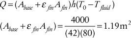

Consider an area of bare surface equal to 10 mm by w or 0.01w. The base area is 0.007w and the equivalent fin area is 2(0.05)w = 0.1w. Normalizing these areas with the bare area gives Abase = Abare(0.007w)/(0.01w) = 0.7Abare and Afin = Abase(0.1w)/(0.01w) = 10Abase. Substitute these values into the above expression, with εfin = 0.90, and solve:

It was pointed out previously that the adiabatic tip assumption for the fin may not be valid and that to account for this, an adjustment in the length of the fin can be made. According to Equation (2.70),
Using this adjusted value of L gives mLc = (11.66)(0.0515) = 0.600 and ɛfin = 0.895 and Afin = 2(0.0515)(w) = 0.103w = 10.3Abase.
Substitute these values into the above expression, with ɛfin = 0.895, and solve:

![]() or a 2% increase from the case when an adiabatic tip is assumed.
or a 2% increase from the case when an adiabatic tip is assumed.
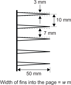
c. The arrangement of the fins is shown in Figure E2.15B.
m = (2h/δk)¼ = [(2)(42)/(0.003)/(206)]¼ = 11.66
L = 0.050 m
mL = 0.5829
From Figure 2.34, ɛfin = 0.86
From Equation (2.74),

Consider an area of bare surface equal to 10 mm by w or 0.01w. The base area is 0.007w, and the equivalent fin area is 2(0.052 + 0.00152)1/2 w ≅ 0.1w. Normalizing these areas with the bare area gives Abase = Abare(0.007w)/(0.01w) = 0.7Abare and Afin = Abase(0.1w)/(0.01w) = 10 Abase. Substitute these values into the above expression, with ɛfin = 0.90, and solve:
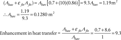
d. From Part (a), A = 1.19 m2—this is equivalent to a length of 1-in tube, Ltube:
e. The arrangement of the fins is shown in Figure E2.15C.

From Figure 2.33, ɛfin = 0.99
From Equation (2.74),
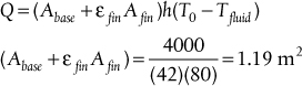
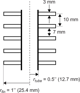
Consider an area of bare surface equal to 10 mm of tube length, Abare = π(0.0254)(0.01) = 7.980 × 10⁻⁴ m. The base area is π(0.0254)(0.007) = 5.586 × 10⁻⁴ m, and the equivalent fin area is 2π(0.02542 − 0.01272)1/2/4 = 7.6 × 10⁻⁴ m. Normalizing these areas with the bare area gives Abase = Abare(5.586 × 10⁻⁴)/(7.980 × 10−4) = 0.7Abare and Afin = Abase(7.6 × 10⁻⁴)/(7.980 × 10−4) = 0.952 Abase. Substitute these values into the above expression, with ɛfin = 0.99, and solve:
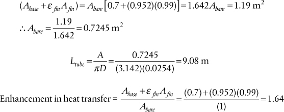
f. The arrangement of the fins is shown in Figure E2.15D.
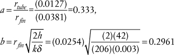
From Figure 2.33, ɛfin = 0.978
From Equation (2.74),
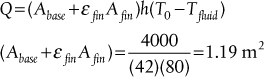
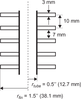
Consider an area of bare surface equal to 10 mm of tube length, Abare = π(0.0254)(0.01) = 7.980 × 10⁻⁴ m. The base area is π(0.0254)(0.007) = 5.586 × 10⁻⁴ m, and the equivalent fin area is 2π(0.03812 − 0.01272)1/2/4 = 20.27 × 10⁻⁴ m. Normalizing these areas with the bare area gives Abase = Abare(5.586 × 10⁻⁴)/(7.980 × 10−4) = 0.7Abare and Afin = Abase(20.27 × 10⁻⁴)/(7.980 × 10−4) = 2.540 Abase. Substitute these values into the above expression, with ɛfin = 0.978, and solve:
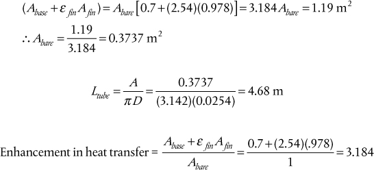
From Example 2.15, it is clear that for all the fins considered, there is a significant enhancement of heat transfer due to the presence of the fins. The enhancement factors for the cases with fins were 10.4, 9.3, 1.64, and 3.184 for cases b, c, e, and f, respectively. The enhancement factor can be considered a measure of the increase in effective film heat transfer coefficient that the fins provide. Thus, the required heat transfer area, based on the base area, is reduced significantly and varies in the range of 40% to 90% reduction for the cases considered in Example 2.15. The choice to use fins is an economic one, since the overall bare heat transfer area will be reduced, but the cost of the heat transfer area increases significantly.
2.7 Algorithm and Worked Examples for the Design of Heat Exchangers
In this section, the theory needed to design a heat exchanger, which has been presented previously, is brought together along with some of the practical considerations of heat-exchanger design. The approach given here is to provide an algorithm to determine a preliminary design of a heat exchanger for a given service. The final design requires the use of sophisticated software and input from a manufacturer of heat exchangers. However, the algorithm presented here should provide a reasonable design, albeit not optimal, for the service considered.
2.7.1 Pressure Drop Considerations
Up until this point, the equations describing the thermal behavior of the heat exchanger have been covered. However, the design of an exchanger is always a compromise in which higher heat transfer coefficients caused by higher fluid velocities are balanced with the high-pressure drops caused by the higher velocities. It is usual in the design process to specify nominal pressure drops for the shell-side and tube-side fluids. Although these nominal values may be exceeded, they usually act as reasonable upper bounds on the allowable pressure drop. The procedure for estimating the pressure drop for the shell-side fluid was covered in Section 2.5.3.2 using Kern’s method. For the tube-side fluid, the standard term for the frictional pressure drop in circular tubes can be used with the addition of four velocity heads per return due to changes in fluid direction for multiple tube passes. The recommended equation is

where Ntp is the number of tube passes, ui is the velocity inside the tubes, and Di is the inside tube diameter. In Equation (2.77), the first term on the right-hand side accounts for the frictional pressure loss in the tubes, and the second term accounts for losses occurring at the ends of the exchanger where the fluid changes direction.
Once a given arrangement of tubes, shells, baffles, and so on, has been made, more sophisticated CFD (computational fluid dynamics) models can be constructed to determine more accurate estimates of the expected pressure drops through the exchanger.
2.7.2 Design Algorithm
The design process for S-T heat exchangers is an iterative one, because the value of U must be known, but it cannot be calculated until values for the shell diameter, baffle spacing, number of tubes, and so on, have been determined, which in turn cannot be calculated unless U is known. Once the calculations have been completed, the assumptions about the construction parameters may be checked and modified and calculations reworked. Following such a process, a final acceptable design can be found. Although not unique, the following algorithm for the design of an S-T heat exchanger is recommended:
1. Establish the energy balance around the heat exchanger:
2. Using the heuristics in Section 2.2.1.7, determine which fluid should go on the shell side and which on the tube side.
3. For the tube side, determine the mass flowrate, inlet temperature, outlet temperature, and enthalpy change.
4. For the shell side, determine the mass flowrate, inlet temperature, outlet temperature, and enthalpy change.
5. Determine all the fluid properties, μ, ρ, k, cp, at the appropriate average temperatures.
6. Determine the maximum allowable pressure drops for the tube side and shell side.
7. Determine the number of shell passes, Nshells, using Equation (2.16) and the number of tube passes, Ntp = 2(or 4 or 6...)Nshells, and determine the LMTD correction factor, FN−2N and LMTD.
8. Choose the shell and tube arrangement. Determine the following:
a. Tube length, Ltube: Standard lengths are 8, 12, 16, and 20 ft
b. Baffle cut, BC: 15% to 45% of Ds with 20% to 35% being “standard”
c. Baffle spacing: Lb ranges from a minimum of 0.2Ds or 2 in to a maximum of Ds
d. Tube diameter, Do: Standard sizes are ¾ and 1 in
e. Tube thickness: Ranges from 12 to 18 BWG (see Table 2.4) and actual value will depend on the tube-side fluid pressure and temperature
f. Tube arrangement (square or triangular) and pitch, p: Typical values are p = 1.25Do for triangular and p = Do + 0.25 in for square
9. Choose a tube-side velocity between 1 and 3 m/s (this should not exceed 3 m/s), and from this value estimate the number of tubes per pass, the total number of tubes in the exchanger, Ntubes, and the inside heat transfer coefficient, hi.
10. Using the tube count information from Tables 2.6 and 2.7, determine the shell diameter.
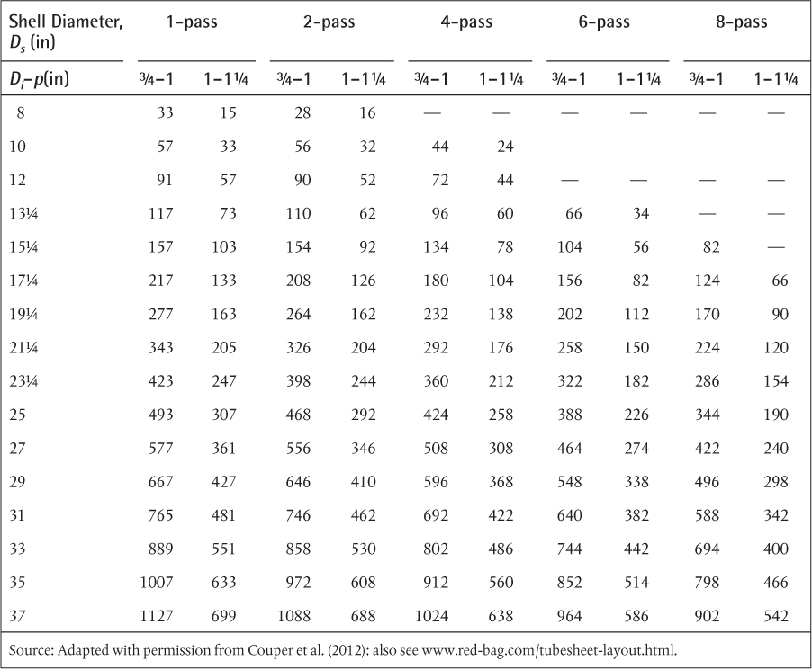
Table 2.6 Tube Counts for Shell-and-Tube Heat Exchangers—Fixed Tubesheet (Equilateral Triangular Pitch)
11. With the shell diameter from Step 10 and the information in Step 8, calculate the shell-side heat transfer coefficient using Equation (2.43).
12. Combine the heat transfer coefficients and fouling and tube metal resistance to give the overall outside heat transfer coefficient, Uo, Equation (2.23).
13. Determine the total heat transfer area required, Ao,new = Q/(UoΔTlmFN−2N) and compare with the total area assumed from Ao = πDoLtubeNtubes.
14. Determine the tube-side and shell-side pressure drops. If either of the pressure drops exceeds the maximum allowable values, adjust the shell/tube configuration to accommodate. Recommended actions include the following:
Tube side: Reduce the tube-side velocity by increasing the number of tubes.
Note that ΔPtube ∝(1/Ntubes)2
Shell side: Increase the baffle spacing or tube pitch.
Note that ΔPshell ∝ (1/Lb)3
If pressure drop is too low, consider increasing the number of tube passes (for increasing ΔPtube) or decreasing the baffle spacing (for increasing ΔPshell). These actions increase the overall heat transfer coefficient, which reduces heat transfer area and the cost of the heat exchanger.
15. Adjust the number of tubes based on the new estimated area and tube-side pressure drop and, if needed, adjust the baffle spacing based on shell-side pressure drop. Iterate from Step 8 until the solution converges—namely, Ao,new in Step 13 is between Ao and 1.2 Ao.
Example 2.16 (Modified from Kern [1950], Example 7.3)
Determine a preliminary rating for a heat exchanger with the following service: 19,900 kg/h of kerosene leaves a distillation column at 200°C and will be cooled to 93°C by 67,880 kg/h of crude oil from storage that is to be heated from 38°C to 76°C. A maximum pressure drop of 70 kPa is permissible for both streams. A scale factor (Rf) of 0.000053m2K/W should be used for this service, which is mainly caused by the crude oil. Based on previous experience, 1-in diameter, 16 ft long, 12 BWG tubes should be used (these may be changed if needed), and the crude oil should flow inside the tubes.
Solution
The steps in the design algorithm are as follows.
1. Energy balance (using average Cp values):

2. Choice of shell- and tube-side fluids:
Set crude in tubes and kerosene in shell since crude is more fouling than kerosene.
3. Tube side—crude oil:

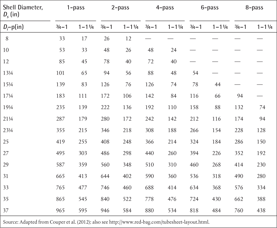
4. Shell side—kerosene:
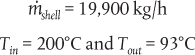
5. Fluid properties:
Crude oil (properties at Tbulk, ave = (38 + 76)/2 = 57°C)
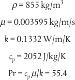
Kerosene (properties at Tbulk, ave = (200 + 93)/2 = 146.5°C)

6. Set maximum pressure drops:
7. Determine the number of shell (Nshells) and tube passes (Ntp):

From Equation (2.16),

The T-Q diagram for this exchanger is shown in Figure E2.16.
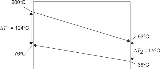

Use Equation (2.13) to determine F1−2:
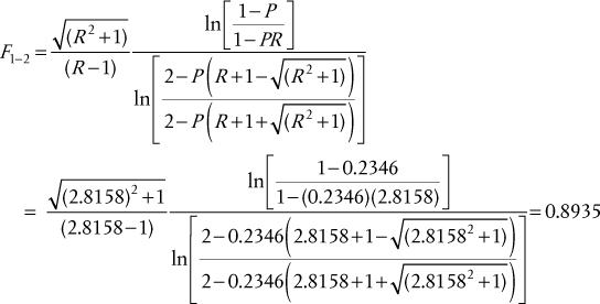
8. Choose shell-and-tube arrangement:
a. Tube length: Ltube = 16 ft = (16)(0.3048) = 4.877 m
b. Baffle cut: BC = 25% of shell diameter, Ds
c. Baffle spacing: Lb = 0.20Ds
d. Tube diameter: Do = 1-in = 0.0254 m
e. Tube thickness: Δxwall for12 BWG (from Table 2.4), tube thickness (Δxwall) = 0.109 in = 0.002769 m
f. Tube arrangement (square or triangular) and pitch, p: Use a square arrangement to allow for cleaning on the outside of the tubes and a pitch of 1.25 in
9. Choose a tube-side velocity and determine number of tubes and tube-side heat transfer coefficient, hi:
ui = 2 m/s. A relatively high velocity is chosen, as the crude is quite viscous and turbulent flow is desired. This can be modified later if the ΔP on the tube side is too high.
A mass balance gives 4

Actual velocity in tubes,
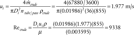
From Equation (2.26),
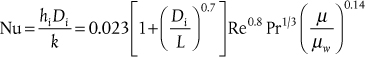
Determine the wall viscosity at an average wall temperature = (146.5 + 57)/2 = 102°C μw,crude = 0.000899 kg/m/s:

10. Determine shell diameter:
For 1-in tubes in a square arrangement with p = 1.25 in, Table 2.7 indicates that a 15¼ in shell diameter will accommodate 76 tubes in a two-pass arrangement.
11. Determine shell-side heat transfer coefficient, ho:
Diameter of shell: Ds = 15.25 in = 0.3874 m
Baffle spacing: Lb = 0.2Ds = (0.2)(0.3874) = 0.07747 m
From Equation (2.37), determine the hydraulic diameter of the shell, DH,s
From Equation (2.41), determine the flow area on the shell side:
Shell-side velocity,
Shell-side Reynolds number,
From Equation (2.43),
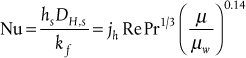
with
The value of μw corresponding to a wall temperature of 102°C is 0.00055 kg/m/s.

12. Combine heat transfer resistance to give Uo:
From Equation (2.23),
Assume the exchanger will be made of carbon steel; from Table 2.3, kw = 45.8 W/m/K (@102°C), and from the problem statement, Rfi = 0.000053 m2K/W:

13. Determine the total heat transfer area required:
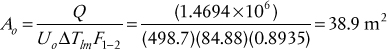
14. Determine the tube-side and shell-side pressure drops:
Tube-side ΔP:
From Equation (2.77), the tube-side pressure loss is given by

where Ntp = 2, ui = 1.977 m/s and f is found from the Pavlov equation (Equation [1.16]),

for drawn tubing, e = 1.5 × 10⁻⁶ m and D = Di = 0.01986 and Re = 9338. Substituting these values into the equation for f gives

This is less than the maximum allowable value of 70 kPa.
Shell-side ΔP:
The shell-side ΔP is obtained from Equation (2.44):

And for Re > 300,
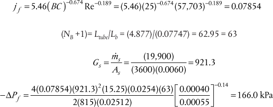
This is greater than the maximum allowable value of 70 kPa.
15. Adjust the number of tubes based on the new estimated area and tube-side pressure drop and, if needed, adjust the baffle spacing based on shell-side pressure drop. Iterate from Step 9 until converged.
Number of tubes:

Because the number of tubes has increased, if the 1–2 configuration is kept, then ΔPtube and hi will both decrease and a solution will not be found. Change the configuration to 1–4.
Shell-side pressure drop:
Using an Lb = 0.2Ds, the value of ΔPshell was 166.0 kPa, which is greater than the maximum allowable value of 70 kPa. Therefore, adjust Lb by a factor = (166.0/70)1/3 = 1.33 so that Lb = (1.33) (0.2Ds) = 0.266Ds, and round up to give Lb = 0.3Ds.
Iterate from Step 9 with Ntubes = 104 (corresponding to 19.25 in shell diameter from Table 2.7) and Lb = 0.3Ds.
The results for the next and subsequent iterations are given in Table E2.16.
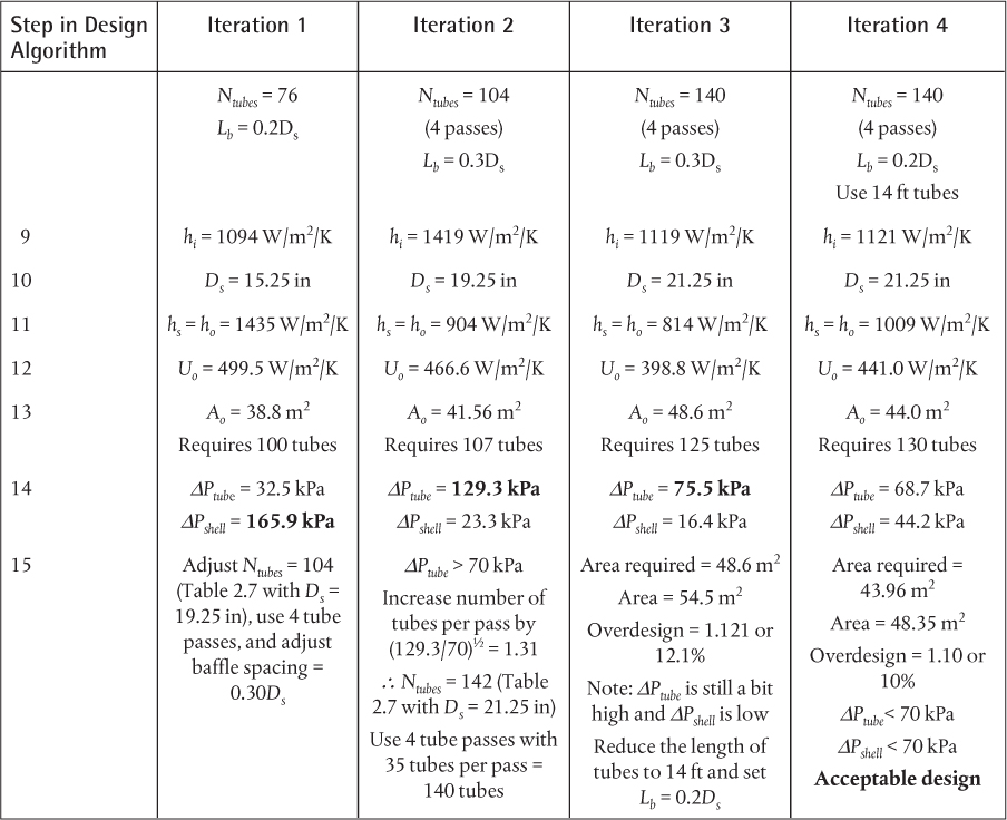
Table E2.16 Results for Worked Example 2.16
The preliminary design for this equipment gives an exchanger with the following specifications:
Number of tubes: 142
Length of Tubes: 14 ft
Tube type: 1-in diameter 12 BWG
Tube arrangement: 1.25-in square pitch
Shell passes: 1; tube passes = 4
Shell diameter: 21.25 in
Baffle cut: 25% of the shell diameter (5.31 in)
Baffle spacing: 20% of the shell diameter (4.25 in)
Overdesign: 10%
2.8 Performance Problems
The main focus of this chapter has been developing the ideas and relationships that describe the heat transfer process in process heat exchangers and then bringing all these ideas together to design a heat exchanger. It has been shown that many, sometimes complex, relationships must be considered in order to design a heat exchanger successfully. However, once the heat exchanger has been designed, built, and installed into a process, further analysis of the heat exchanger is still necessary. As any process engineer will attest, a heat exchanger (or any other piece of process equipment) will hardly ever (never) run under the exact conditions for which it was designed. This does not mean that the design algorithm or any of the calculations were incorrect but rather that the heat exchanger is now part of a complex chemical process with the main objective to make profitable chemicals from less-expensive feed stocks. Therefore, in the day-to-day operations of the plant, things will change almost continuously, and the heat exchanger will have to operate over a spectrum of conditions in order for the process to produce the desired amount of product chemicals.
An example of off-design conditions will occur when there is high market demand for the chemical(s) produced from a process. Under these conditions, the process may have to be run to maximize the products (and profits) from the plant. Thus, the process might be pushed to 110% or 120% of its design capacity. Obviously, every heat exchanger in the plant will be operating quite far from its design conditions. The opposite might occur when there is weak market demand. The question addressed in this section is, for a given existing heat exchanger, how is the performance of that heat exchanger predicted?
2.8.1 What Variables to Specify in Performance Problems
When determining the performance of an existing heat exchanger, the same equations that were used in the design must be solved, specifically, the enthalpy balances for both streams and the design equation Q = UAΔTlmF. However, unlike in the design calculation, the conditions of the streams leaving the exchanger are usually unknown, but the conditions entering are known. In addition, the size (heat transfer area) is known and fixed. For example, consider the exchanger designed in Section 2.7.2. This exchanger was built as specified and has been operating in the plant. The current operating conditions are
It should be noted that these conditions are not the design conditions because the exchanger was built with approximately 10% additional area required to perform the design. Thus, more heat is transferred between the streams, and the crude leaves hotter and the kerosene leaves cooler than the design specification, which is to be expected because of the overdesign.
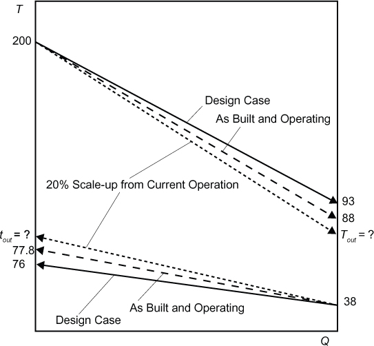
Now consider the case when the plant is to be scaled up. It is desired that the flows of crude and kerosene be increased by 20%. If the temperatures into the exchanger remain the same as in the design case, the exit temperatures of both streams must be determined. This problem is illustrated in Figure 2.36. For performance problems (where the equipment has been designed, installed, and is operating), the easiest way to determine the new operating conditions is via a ratio analysis, shown in the next section. The terms rating and performance are synonymous when considering how existing equipment performs. However, the term performance problem is preferred in this text.
2.8.2 Using Ratios to Determine Heat-Exchanger Performance
From the problem given in Example 2.16, it is clear that the design of the exchanger is quite involved. Rather than revisit all the equations used in this example, a simpler approach is adopted for evaluating the performance problem. As was explained in Chapter 1, the idea is to take the ratio of the important equations describing the heat transfer process; that is, the two enthalpy balances and the design equation for the new case (subscript 2) and the base case (subscript 1). Thus,

If there are changes in phase, the enthalpy balances will have heats of vaporization instead of sensible heats, but the approach is similar. The assumption is then made that, for relatively small changes in flows, the physical properties of the fluids remain constant and also that the LMTD correction factors remain constant. The validity of these assumptions can be checked later. For the problem considered here, the three equations can be rewritten:


In Equations (2.81), (2.82), and (2.83), the ratios of the crude oil and kerosene flowrates for cases 1 and 2 are given as m and M, respectively. For the case of 20% scale-up, these ratios are 1.2 each. The ratio of the heat transferred is designated as Q, but it should be noted that Q is not 1.2 and must be determined.
In Equation (2.83), the ratio of the overall heat transfer coefficients must be determined. For the base case, from the last iteration in Table E2.16, ho = 1009 W/m2/K, hi 1121 W/m2/K, and


In Equation (2.84), the inside (tube) and outside (shell) heat transfer coefficients are dependent on the flows of the tube- and shell-side fluids. From Equations (2.27) and (2.36) for turbulent flow in the tubes and the shell, the heat transfer coefficients are related to the mass flow of fluids through the Reynolds number as follows:
It should be noted that in Kern’s method, the exponent on the Reynolds number is a little below 0.6, but this difference is small, and 0.6 can be used for shell-side flow. Using these relationships and noting that for constant physical properties Re is proportional to the mass flowrate, Equation (2.84) may be rewritten for the new case as

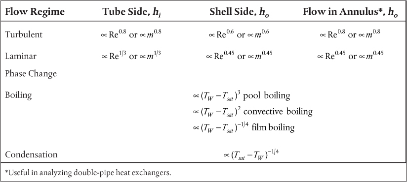
Substituting Equations (2.85) and (2.86) in (2.83) gives
Equations (2.81), (2.82), and (2.87) may now be solved simultaneously to give
Thus, the crude temperature decreases from 77.8°C to 76.4°C, and the kerosene temperature increases from 88°C to 91.3°C. Clearly, the average fluid properties would not change significantly for these temperature changes; similarly, the value of the LMTD correction factor hardly changes from 0.894 to 0.885, a change of ~1%. It should also be noted that the amount of heat transferred between the streams increases by only 16.5%, because the heat transfer coefficients are not linearly dependent on the mass flow rates.
Table 2.8 gives the dependence of individual heat transfer coefficients on the mass flow rate (effectively the Reynolds number, Re). Also shown in Table 2.8 are the relationships to be used when phase changes are considered. For phase changes, the mass flow rates do not affect the heat transfer coefficients, but the ΔT between the wall and fluid may be important.
2.8.3 Worked Examples for Performance Problems
To reinforce the concepts introduced in the preceding section, some worked examples are provided.
An S-T exchanger is designed to exchange heat between two process streams. The T-Q diagram is shown in Figure E2.17. The inside and outside heat transfer coefficients are equal (hi = ho = 1000 W/m2/K). If the shell-side fluid flow rate is increased by 25% and the tube-side flow and the temperatures of both streams entering the heat exchanger remain unchanged, calculate
a. The outlet temperatures of both streams assuming that the service is non-fouling and that the tube wall is thin and offers negligible heat transfer resistance.
b. The outlet temperatures of both streams assuming that the service is non-fouling and the tubes are 1-in, 14-BWG and made of copper.

Solution
a. For the design case (Case 1),
The ratio form of the energy balance and design equations are


where

and using the relationships from Table 2.8,

Substituting Equations (E2.17f) and (E2.17g) into (E2.17e) gives

Solving Equations (E2.17c), (E2.17d), and (E2.17h) simultaneously gives
b. Di = 0.02118 m, Do = 0.0254, kw = kcopper = 380 W/m/K
For the design case (Case 1),

The ratio form of the energy balance and design equations are

where

Substituting Equations (E2.17i), (E2.17j), (E2.17n), and (E2.17o) into (E2.17m) and solving (E2.17k), (E2.17l), and (E2.17m) gives
These results are virtually the same as for Part (a), which is not surprising, since the resistance due to the conduction through the wall can often be neglected.
A hot, viscous process stream is cooled using cooling water (cw). The exchanger is a double-pipe design in which the cooling water flows in the annulus and the viscous process fluid flows in the inner pipe. The T-Q diagram for the exchanger at design conditions is shown in Figure E2.18 along with an image of a double-pipe exchanger. At design conditions, the cw is in the turbulent regime, but the process fluid is in the laminar flow regime. The process is to be scaled down such that the process flow is reduced to 72% of its current value, but the inlet temperature is maintained at 95°C. It is desired to keep the exit temperature of the process at the current value of 55°C by reducing the cooling water flow rate. However, the maximum temperature of the cooling water is set at 45°C because, if it gets hotter than this value, then excessive scaling of the heat exchanger will result.
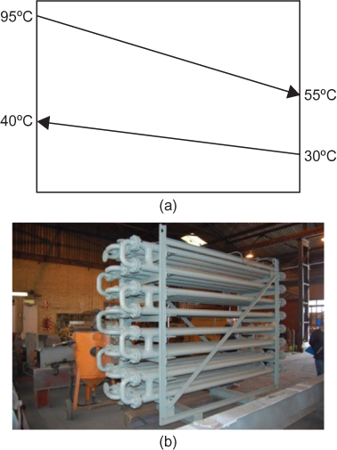
Figure E2.18 T-Q diagram for design case and photo of a double-pipe heat exchanger (Courtesy of Protherm Systems [Pty] Ltd., www.protherm.co.za/product/protherm-shell-tube-heat-exchangers)
Data:
hi = 125 W/m2/K
ho = 3500 W/m2/K
Ro = 1.76 × 10⁻⁴ m2/K/W, Ri = 0
Inner tube = 0.75-in, 16-BWG copper (Di,i = 0.01576 m Di,o = 0.01905 m)
Outer tube = 1.25-in, 16-BWG copper (Do,i = 0.02845 m Do,o = 0.03175)
kcopper = kw = 380 W/m/K
a. Can this operation be accomplished? Determine the cw flow rate and exit temperature of cw.
b. If the desired reduction in process flow rate cannot be achieved, determine the minimum process flow rate and the cw flow rate to accomplish this.
Solution
a. For the design (base case or Case 1) condition,
and

For the scaled down case (Case 2), the unknowns are the new cooling water flowrate, ![]() 2, and the cooling water outlet temperature, t2. Using the relationships in Table 2.8, the value of U2 is given by
2, and the cooling water outlet temperature, t2. Using the relationships in Table 2.8, the value of U2 is given by

The energy balance and design equations (noting that for a double-pipe heat exchanger the flow is pure countercurrent and F = 1) are


where
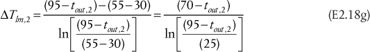
Substituting Equations (E2.18a), (E2.18b), (E2.18c), and (E2.18g) into (E2.18f) and solving Equations (E2.18d), (E2.18e), and (E2.18f) simultaneously gives
This solution is not practical, since reducing the cooling water flow to 28.4% of the design case increases the exit temperature to well above 45°C, and excessive fouling of the exchanger would result. This fouling is due to the reverse solubility of many of the salts found in water, which start to precipitate out at temperatures greater than 45°C.
b. The unknown variables now become the process flowrate and the cooling water flowrate (i.e., m and M). In addition, the exit temperature of the cooling water is set to 45°C, which is the maximum allowable temperature.
The ratio form of the energy balance and design equations are


where
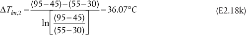
and
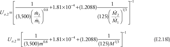
Substituting Equations (E2.18k) and (E2.18l) into (E2.18j) and solving (E2.18h), (E2.18i), and (E2.18j) simultaneously gives
Thus, the maximum scale-down is a little less than 10%, and the cw flowrate must be reduced to 60.43% of the design value.
It is important to note the implications of this result on the control and flexibility of operation for this process. If scale-down below 10% is required, then the only feasible way to achieve this is for the process temperature to drop below 55°C. This may not be a problem, but if, for example, the viscosity of the process fluid became too large at temperatures less than 55°C, then this design would need to be changed.
A reboiler for a column is supplied with saturated steam (in shell) at a temperature of 145°C and reboils the bottom product (in tubes) that leaves the column at 122°C. It is desired to increase the boil-up rate by 15% from the design case. How can this change be accomplished?
Solution
The T-Q diagram for the current operation of the reboiler is shown in Figure E2.19.
In looking at the relevant relationships, Equations (2.78), (2.79), and (2.80), and noting that the heats of vaporization will not change, that the area of the exchanger is constant, and the LMTD correction factor, F = 1:

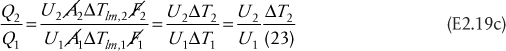

From Table 2.8, it can be seen that neither the condensing- nor the boiling-side coefficients are a function of flowrate. Thus, ignoring the effects of the changing wall temperature, U2/U1 = 1. This reduces Equation (E2.19c) to
It must be concluded that the only way to increase the boil-up rate by 15% (i.e., Q2/Q1 = 1.15) is to increase ΔT2 to (1.15)(23) = 26.45°C. This would most likely be done by increasing the steam temperature (and pressure) to 148.45°C. Alternatively, the column pressure could be lowered to bring the temperature of the boiling process liquid in the reboiler down to (122 − 3.45) = 118.55°C. However, that would involve decreasing the pressure at which the column operates, which might not be possible or desirable.
This solution is not quite correct, since the temperature driving forces for boiling and condensation will change slightly, that is, the wall temperature will change. In order to find the change in the wall temperature, the relative magnitudes of the condensing and boiling heat transfer coefficients must be known. This problem is considered in the next example.
Revisiting Example 2.19, by how much should the steam temperature be increased in order to achieve the 15% increase in boil-up rate for the case when the process- and steam-side heat transfer coefficients are approximately equal?
Assume that this is a non-fouling service, the conduction resistance of the tube wall may be assumed negligible, and Di ≅ Dod. In addition, the process fluid may be assumed to be in the convective boiling regime.
Solution
For the original design case, Equation (2.23), reduces to
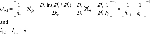
Writing an energy balance across the inside and outside films gives
For the new case (15% scale-up), the energy balance becomes
The design relationship for this case is

and from Table 2.8, U2 can be written in terms of the temperature driving forces as

Substituting the relationships for ho,2 and hi,2 from Table 2.8 in Equation (E2.20b) gives
Substituting Equation (E2.20d) into (E2.20c) and solving the resulting equation simultaneously with Equation (E2.20e) gives the two unknowns, Tsteam, 2 and Tw, 2:
Note that the answer differs only a small amount from that obtained in Example 2.19 where Tsteam, 2 = 148.45°C.
It should be noted that in Example 2.20, an additional relationship was used, namely, a flux balance across the wall given by Equations (E2.20a) and (E2.20b), in order to determine the unknown wall temperature Tw. The final problem considers a situation where the heat transfer coefficients and exchanger area are unknown, but one heat transfer coefficient is known to be limiting.
A condenser is used to condense saturated steam to saturated liquid at 150°C (shell) using a process stream entering at 30°C and exiting at 50°C (tubes). Assume that the condensation resistance is negligible compared to that of the process stream. The condensation throughput must be decreased by 50%. By what factor must the flowrate of the process stream be reduced?
The T-Q diagram for this problem is shown in Figure E2.21.
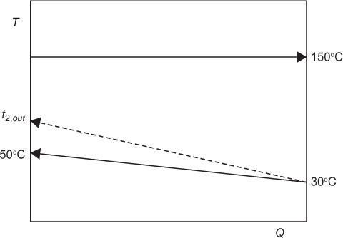
Solution
In this problem, the area and heat transfer coefficients are not known; nevertheless, there is sufficient information to solve the problem.


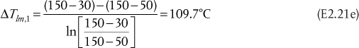
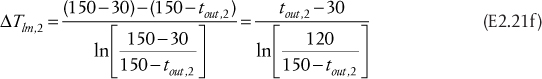
Substituting Equations (E2.21d), (E2.21e), and (E2.21f) into Equation (E2.21c) gives
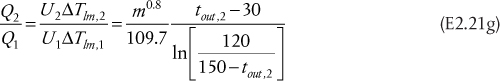
Solving Equations (E2.21a), (E2.21b), and (E2.21g) simultaneously gives tout,2= 53.3°C, m = 0.4291 or reduce the process stream to 42.91% of design flowrate.
Notation


Subscripts

References
Bell, K. J., and A. C. Mueller. 2014. Wolverine Engineering Data Book II. Ulm, Germany: Wieland-Werke AG. http://ichemengineer-heattransfer.blogspot.com/2014/11/wolverine-heat-transfer-data-book-ii-by.html.
Bennett, C. O., and J. E. Myers. 1983. Momentum, Heat, and Mass Transfer, 3rd ed. New York: McGraw-Hill.
Bowman, R. A. 1936. “Mean Temperature Difference Correction in Multipass Exchangers.” Ind Eng Chem 28: 541–544.
Bowman, R. A., A. C. Mueller, and W. M. Nagle. 1940. “Mean Temperature Difference in Design.” Trans ASME 62: 283–294.
Bromley, L. A. 1950. “Heat Transfer in Stable Film Boiling.” Chem Eng Progr 46: 221–227.
Chen, C. Y., G. A. Hawkins, and H. L. Solberg. 1946. “Heat Transfer in Annuli.” Trans ASME 68: 99–106.
Churchill, S. W., and M. Bernstein. 1977. “A Correlating Equation for Forced Convection from Gases and Liquids to a Circular Cylinder in Crossflow.” J Heat Transfer, Trans ASME 99: 300–306.
Cichelli, M. T., and C. F. Bonilla. 1945. “Heat Transfer to Liquids Boiling Under Pressure.” Trans Am Inst Chem Engrs 41: 755–787.
Clark, S. H., and W. M. Kays. 1953. “Laminar Flow Forced Convection in Rectangular Ducts.” Trans ASME 75: 859–866.
Cooper, M. G. 1984. “Saturated Nucleate Pool Boiling—A Simple Correlation.” First UK National Heat Transfer Conf., IChemE Symp Ser, No. 86, 2, 785–793.
Couper, J. R., W. R. Penney, J. R. Fair, and S. M. Walas. 2012. Chemical Process Equipment—Selection and Design, 3rd ed. Oxford, UK: Butterworth-Heinmann.
Dittus, F. W., and L. M. K. Boelter. 1985. “Heat Transfer in Automobile Radiators of Tubular Type.” Int Comm Heat Mass Transfer 12: 3–22; modified from Univ. Calif. Publ. in Engineering 2: 443–461 (1930).
Geankoplis, C. J. 2003. Transport Processes and Separation Process Principles, 4th ed. Upper Saddle River, NJ: Prentice Hall.
Green, D. W., and R. H. Perry. 2008. Perry’s Chemical Engineers’ Handbook, 8th ed. New York: McGraw-Hill.
Gungor, K. E., and R. H. S. Winterton. 1986. “A General Correlation for Flow Boiling in Tubes and Annuli.” Int J Heat Mass Transfer 29: 351–358.
Hausen, Z. 1943. Ver Deut Beth Verfahrenstech 4: 91.
Kern, D. Q. 1950. Process Heat Transfer. New York: McGraw-Hill.
McAdams, W. H. 1954. Heat Transmission, 3rd ed. New York: McGraw-Hill.
Mukherjee, R. 1998. “Effectively Design Shell-and-Tube Heat Exchangers.” Chem Eng Prog 2: 21–37.
Rohsenow, W. M. (Ed.). 1964. Developments of Heat Transfer. Cambridge, MA: MIT Press.
Shelton, S. M. “Thermal Conductivity of Some Irons and Steels over the Temperature Range 100 to 500°C.” J Res Nat Stand 12 (April 1934).
Sieder, E. N., and G. E. Tate. 1936. “Heat Transfer and Pressure Drop of Liquids in Tubes.” Ind Eng Chem 28: 1429–1435.
Tinker, T. 1958. “Shellside Characteristics of Shell-Tube Heat Exchangers—A Simplified Rating System for Commercial Heat Exchangers.” Trans ASME 80: 36–52.
Tubular Exchanger Manufacturers Association. 2013. Standards of the Tubular Exchanger Manufacturers Association, 9th ed. Tarrytown, NY: Tubular Exchanger Manufacturers Association.
Žukauskas, A. 1972. “Heat Transfer from Tubes in Crossflow.” Advances in Heat Transfer 8: 93–160.
Zuber, N. 1958. “On the Stability of Boiling Heat Transfer.” Trans ASME 80: 711.
Appendix 2.A Heat-Exchanger Effectiveness Charts
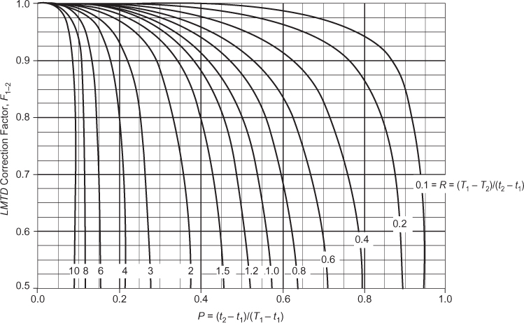

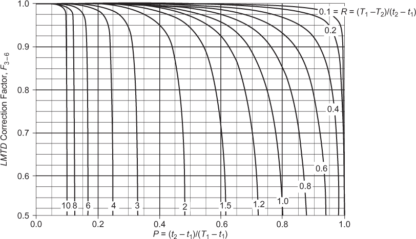
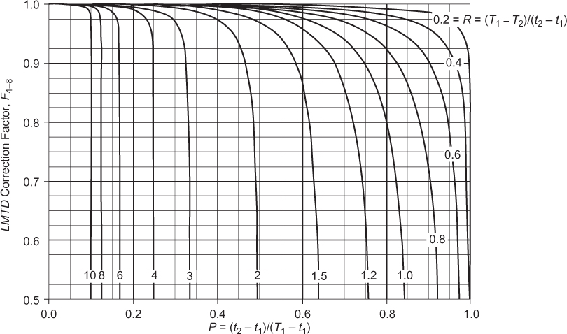

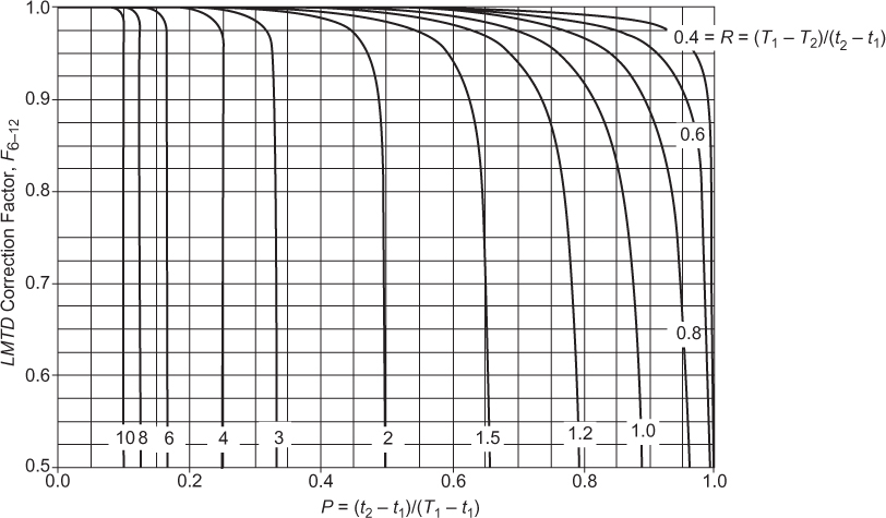

Figure A.7 LMTD correction factors for a 1–1 cross-flow heat exchanger with both fluids unmixed (use this for air coolers with a single tube pass)
For LMTD correction factors for other configurations, see CheCalc’s LMTD Correction Factor Charts at http://checalc.com/solved/LMTD_Chart.html.
Appendix 2.B Derivation of Fin Effectiveness for a Rectangular Fin
Rectangular Fin with Constant Thickness
The heat transfer process occurring in the fin consists of conduction through the fin and convectional loss from the side of the fin. The geometry and notation used in this derivation are shown in Figure B.1. A differential flux balance on a slice through the fin yields
where W is the width of the fin, δ is the fin thickness, h is the heat transfer coefficient between the fin and the surrounding fluid, and Tfluid is the temperature of the surrounding fluid. Equation (B.2.1) means that the heat flow into a differential section of the fin by conduction equals the heat flow out of the differential section of the fin by conduction down the length of the fin plus the heat exchanged with the surroundings in that differential section of the fin by convection. It is important to remember that heat is exchanged with the surroundings on both the top and bottom faces of the fin. Dividing through by δWΔx and taking the limit as Δx → 0 yields the following differential equation:
Substituting Fourier’s law of heat conduction ![]() in Equation (B.2.2) gives
in Equation (B.2.2) gives
Introducing the new variable T′ = Tx − Tfluid gives

The boundary condition at x = 0 is T = T0 or T′ = T0 − Tfluid. Several possible boundary conditions exist for x = L, the simplest being that dT′/dx = 0, which means that there is no heat lost from the tip of the fin (adiabatic fin tip). This is a good approximation for the case where the tip of the fin has a very small surface area compared to the faces of the fin. The second boundary condition is reasonable and accurate for long, thin fins, but for short thick fins, the amount of heat lost from the fin tip may be significant. Nevertheless, the adiabatic fin tip assumption may be used for all types of fin with an adjustment that is discussed in Section 2.6. With these boundary conditions, Equation (B.2.4) can be integrated as follows:

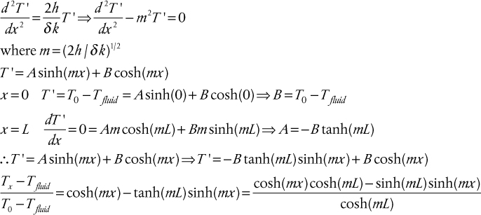

The total heat transferred into the fin is (δW)qx=0 or

At this point, the efficiency of the fin is introduced and is defined as

Substituting the result from Equation (B.2.6) into Equation (B.2.7) gives

This result is plotted in Figure 2.32.
Problems
Short Answer Problems
1. Why is it necessary to include an LMTD correction factor (F) into the design equation for most practical heat exchangers?
2. Explain why you agree or disagree with this statement: Because the heat transfer coefficients for gases are always much lower than for liquids, the limiting resistance for condensers (where a gas is turned into a liquid) is always on the condensing side of the heat exchanger.
3. For shell-and-tube exchangers in which the flow is turbulent and there is no phase change taking place for either stream, how does the heat transfer coefficient change with a 50% increase in the mass flowrate for the
a. Shell-side fluid?
b. Tube-side fluid?
4. Repeat Problem 2.3 assuming laminar flow for both fluids.
5. Would you expect the heat transfer coefficient for a given fluid to be higher if the fluid were in laminar flow or turbulent flow? Explain your answer.
6. Give three reasons for placing a specific fluid on the tube side of an S-T heat exchanger.
7. Give three reasons for placing a specific fluid on the shell side of an S-T heat exchanger.
8. Why are fins (extended surfaces) used in some heat exchangers?
9. Give explanations for the following terms for S-T heat exchangers:
a. Baffle cut
b. Number of tube passes
c. Tube pitch
d. Tube arrangement
10. State the basic design equation for an S-T heat exchanger in which there are no phase changes, and draw a sketch of the T-Q diagram with the relevant terms shown.
11. Draw the T-Q diagram for the following cases:
a. Condensing (pure) vapor using cooling water
b. Distillation reboiler using condensing steam as the heating media
c. Process liquid stream cooled by a another process stream
Problems to Solve
12. A process fluid (Stream 1) (Cp = 2100 J/kg/K) enters a heat exchanger at a rate of 3.4 kg/s and at a temperature of 135°C. This stream is to be cooled with another process stream (Stream 2) (cp = 2450 J/kg/K) flowing at a rate of 2.65 kg/s and entering the heat exchanger at a temperature of 55°C. Determine the following (you may assume that the heat capacities of both streams are constant):
a. The exit temperature of Stream 1 if pure countercurrent flow occurs in the exchanger and the minimum approach temperature between the streams anywhere in the heat exchanger is 10°C
b. The exit temperature of Stream 1 if pure cocurrent flow occurs in the exchanger and the minimum approach temperature between the streams anywhere in the heat exchanger is 10°C
13. Repeat Problem 2.12 for the case when the specific heat capacities of both streams vary linearly with temperature with the following values:
a. Stream 1: Cp = 2000 + 3(T − 100) J/kg/K
b. Stream 2: cp = 2425 + 5(T − 50) J/kg/K
14. The T-Q diagrams for three S-T heat-exchanger designs are given in Figure P2.14(a–c). Determine the number of S-T passes required to accomplish these designs.
15. At a given point in a thin-walled heat exchanger, the shell-side fluid is at 100°C and the tube side fluid is at 20°C. Ignoring any fouling resistances and the resistance of the wall, determine the wall temperature for the following cases:
a. The inside and outside heat transfer coefficients are equal.
b. The inside coefficient has a value 3 times that of the outside coefficient.
c. The inside coefficient has a value ⅓ that of the outside coefficient.
d. The inside coefficient is limiting.
16. In a heat exchanger, water (cp = 4200 J/kg/K) flows at a rate of 1.5 kg/s, and toluene (cp = 1953 J/kg/K) flows at a rate of 2.2 kg/s. The water enters at 50°C and leaves at 90°C, and the toluene enters at 190°C. For this situation, do the following:
a. Sketch the T–Q diagram if the flows are countercurrent.
b. Sketch the T–Q diagram if the flows are concurrent.
17. At a given location in a double-pipe heat exchanger, the bulk temperature of the fluid in the annulus is 100°C, and the bulk temperature of the fluid in the inner pipe is 20°C. The tube wall is very thin, so the resistance due to the metal wall may be ignored. Likewise, fluid fouling resistances may also be ignored. The individual heat transfer coefficients at this point in the heat exchanger are
a. What is the temperature of the wall at this location?
b. What is the heat flux across the wall at this location?
c. If there was a fouling resistance of 0.001 m2K/W on the inside surface of the inner pipe, what would the temperature of the wall be at this location?
18. A single phase fluid (![]() and cp = 1800 J/kg/K) is to be cooled from 175°C to 75°C by exchanging heat with another single phase fluid (
and cp = 1800 J/kg/K) is to be cooled from 175°C to 75°C by exchanging heat with another single phase fluid (![]() and cp = 2250 J/kg/K), which is to be heated from 50°C to 150°C. You have the choice of one of the following five heat exchangers:
and cp = 2250 J/kg/K), which is to be heated from 50°C to 150°C. You have the choice of one of the following five heat exchangers:
Which exchanger do you recommend using for this service? Carefully explain your answer.
(For the following problems and where information on organic materials is not given in the problem, the physical properties may be obtained from a process simulator using the SRK thermodynamics package or from using suitable handbooks.)
19. What is the critical nucleate boiling flux for water at 20 atm?
20. Water flows inside a long ¾-in, 16 BWG tube at an average temperature of 110°F. Determine the inside heat transfer coefficient for the following cases:
a. Velocity = 0.1 ft/s
b. Velocity = 3 ft/s
21. Use Equations (2.47) and (2.48) to estimate the heat flux and heat transfer coefficient for boiling acetone at 1 atm pressure for a temperature driving force of 10°C. You may assume a Cf value of 0.01 for this problem.
22. Use the Sieder-Tate equation to determine the inside heat transfer coefficient for a fluid flowing inside a 16 ft long, 1-in tube (14 BWG) at a velocity of 2.5 ft/s that is being cooled and has an average temperature of 176°F and an average wall temperature of 104°F. Consider the following fluids:
a. Acetone (liquid)
b. Isopropanol (liquid)
c. Methane at 1 atm pressure—use a velocity of 50 ft/s
d. Compare the results from Parts (a), (b), and (c) using the Dittus-Boelter equation
23. Water at 5 atm pressure and 30°C flows at an inlet velocity of 1 m/s into a square duct 2.5 m long that has a cross section of 25 mm by 25 mm. The wall of the duct is maintained at a temperature of 120°C by condensing steam. What will the temperature of the water be when it exits the duct?
24. An S-T condenser contains six rows of five copper tubes per row on a square pitch. The tubes are ¾-in, 14 BWG, and 3 m long. Cooling water flows through the tubes such that hi = 2000 W/m2/K. The water flow is high so that the temperature on the tube side may be assumed to be constant at 35°C. Pure, saturated steam at 2 bar is condensing on the shell side. Determine the capacity of the condenser (Q in kW) if the condenser tubes are oriented (a) vertically, and (b) horizontally.
25. Liquid dimethyl ether (DME) flows across the outside of a bank of tubes. It enters at 100°C and leaves at 50°C. The DME enters at a flowrate of 20 kg/s, the shell diameter is 15 in, the baffle spacing is 6 in, the baffle cut (BC) is 15%, and 1-in OD tubes on a 1.25-in pitch are used. The fluid (cooling water) inside the tubes may be assumed to be at a constant temperature of 35°C and the inside coefficient is expected to be much higher than the shell-side coefficient, and thus the wall temperature may be taken as 35°C.
Use Kern’s method to determine the average heat transfer coefficient for the shell side for the following arrangements:
a. Square pitch
b. Equilateral triangular pitch
26. A double-pipe heat exchanger consists of a length of 1-in, schedule-40 pipe inside an equal length of 3 in, schedule-40 pipe. Water flows at a velocity of 1.393 m/s in the annular region between the pipes and enters the heat exchanger at 30°C. Oil flows in the inner pipe at an average velocity of 1 m/s and enters at 100°C. The water and oil flow countercurrently. Following are the properties of the water and oil:
Determine how long the pipe lengths must be in order for the oil to leave the exchanger at 50°C. You may assume that both fluids are clean and that there is no fouling or tube wall resistances.
27. A 3 m long, 1.25-in, BWG 14 copper tube is used to condense ethanol at 3 bar pressure. Cooling water at 30°C flows through the inside of the tube at a high rate such that the wall temperature may be assumed to be 30°C and the inside heat transfer coefficient may be assumed to be much greater than the outside coefficient. Determine how much vapor will condense (kg/h) assuming no fouling resistance for the following cases:
a. The tube is oriented vertically.
b. The tube is oriented horizontally.
28. Air (1 atm and 30°C) flows crosswise over a bare copper tube (1-in, BWG 16). The approach velocity of the air is 20 m/s. Water enters the tube at 140°C and leaves the tube at an average temperature of 80°C. The average velocity of the water in the tube is 1 m/s. Determine the length of tube required to cool the water to the desired 80°C.
29. Oil flows inside a thin-walled copper tube of diameter Di = 30 mm. Steam condenses on the outside of the tube, and the tube wall temperature may be assumed to be constant at the temperature of the steam (150°C). The oil enters the tube at 30°C and a flow rate of 1.6 kg/s. The properties of the oil are as follows:

a. Calculate the inside heat transfer coefficient, hi, using the appropriate correlation. You should assume that the bulk oil temperature changes from 30°C to 50°C along the tube.
b. Using the result from Part (a), calculate the length of tube required to heat the oil from 30°C to 50°C.
30. Use the approach given in Example 2.12 to determine the length of tubes necessary to vaporize an organic liquid (acetic acid at 1 bar) flowing inside a set of vertical ¾-in, BWG 16 tubes using condensing steam on the outside of the tubes to provide the energy for vaporization. The major resistance to heat transfer is expected to be on the inside of the tubes, and the wall temperature, as a first approximation, may be assumed to be at the temperature of the condensing steam, which for this case is 125°C. It may be assumed that the value of the vapor quality, x, varies from 0.05 to 0.95 in the tube. The physical parameters for acetic acid are
ρv = 1.893 kg/m3, ρl = 939.7 kg/m3, μv = 11.32 × 10⁻⁶ kg/m/s, μl = 390.1 × 10⁻⁶ kg/m/s, Tsat = 117.6°C, Pc = 57.9 bar, M = 60, kl = 0.1423 W/m/K, λ = 405 kJ/kg, cp,l = 2.434 kJ/kg/K, cp,v = 1.319 kJ/kg/K, λ = 0.04 kg/s/tube
31. Repeat Problem 2.28 to find the length of a tube fitted with 2-in diameter, 1/16-in thick annular fins spaced a distance of 3/16-in apart.
32. An air heater consists of a shell-and-tube heat exchanger with 24 longitudinal fins on the outside of the tubes. The tubes are 1.5-in, 14 BWG, and the fins are 0.75 mm thick and are 15 mm long. A total of 8 fins are spaced uniformly around the circumference of each tube. The tubes are made from carbon steel, and their length is 3 m. Air at 0.8 kg/s is being heated from 30°C to 200°C in the shell, and the heat transfer coefficient may be taken as ho = 25 W/m2/K (without fins). Steam is condensing at 254°C in the tubes, and at that temperature λ = 1700 kJ/kg. The tube-side heat transfer coefficient may be taken as hi = 6000 W/m2/K, and no fouling occurs for this service.
a. Calculate the overall heat transfer coefficient with and without fins.
b. Calculate the heat transfer area and the number of tubes needed with and without fins.
33. Your assignment is to design a replacement condenser for an existing distillation column. Space constraints dictate a vertical-tube condenser with a maximum height (equals tube length) of 3 m. An organic is condensed at a rate of 12,000 kg/h at a temperature of 75°C, and cooling water is used, entering at 30°C and exiting at 40°C. The person you are replacing has done some preliminary calculations suggesting that a 1–4 exchanger (water in tubes) using 1-in 16 BWG copper tubes on 1.25-in equilateral triangular pitch with a 37-in shell diameter would be suitable. However, there are only partial calculations to support this claim, and the person who performed the original design is unavailable for consultation. Complete the detailed heat transfer calculations to evaluate the suitability of this heat-exchanger design.
Data for condensing organic:
ρf = 800 kg/m3
ρg = 5.3 kg/m3
λ = 800 kJ/kg
cpl = 2600 J/kg/K
kf = 0.15 W/m/K
μf = 0.4 × 10⁻³ kg/m/s
Heat transfer coefficient for tube side: 6000 W/m2/K
Typical fouling coefficient for plant cooling water: 1200 W/m2/K (=1/Rfi)
Assume no fouling on condensing side
34. A 1–2 shell-and-tube heat exchanger has the following dimensions:
Tube length: 20 ft
Tube diameter: 1-in, BWG 14 carbon steel (kcs = 45 W/m/K)
Number of tubes in shell: 608
Shell diameter: 35 in
Tube arrangement: Triangular pitch, center-to-center = 1.25 in
Number of baffles: 19
Baffle spacing: 1 ft
Baffle: Horizontal baffle with baffle cut = 25%
The fluids in the shell and tube sides of the exchanger have the following properties:

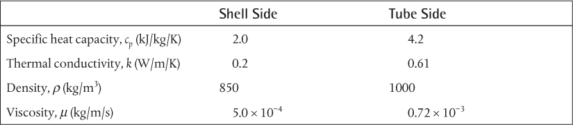
It may be assumed that neither fluid changes phase, and the viscosity correction factor at the wall may be ignored for both fluids. Determine the following:
a. The inside heat transfer coefficient
b. The shell-side heat transfer coefficient
c. The overall heat transfer coefficient (assuming that fouling may be ignored)
d. The exit temperatures of both fluids
35. A 1–2 S-T heat exchanger is used to cool oil in the tubes from 91°C to 51°C using cooling water at 30°C. In the design case, the water exits at 40°C. The resistances on the water and oil sides are equal. What are the new cooling water outlet temperature and the required cooling water flowrate if the oil throughput must be increased by 25% but the outlet temperature must be maintained at 51°C?
36. Repeat Problem 2.35 if the oil side provides 80% of the total resistance to heat transfer.
37. Repeat Problem 2.35 for the case when the oil throughput must be increased by 25% but the cooling water flow rate remains unchanged from the base case. Determine the new outlet temperatures for both the process and cooling water streams?
38. For the situation in Problem 2.35, suppose that the flowrate of the process stream must be reduced while keeping the process exit temperature at 51°C. Therefore, it will be necessary to reduce the flow of the cooling water stream. Determine the maximum scale-down of the process fluid that can occur without the exit cooling water temperature exceeding the limit of 45°C (when excessive fouling is known to occur). Plot the results as the ratio of the process stream flowrate to the base case value (x-axis) versus the cooling water exit temperature.
39. A reboiler is a heat exchanger used to add heat to a distillation column. In a typical reboiler, an almost pure material is vaporized at constant temperature, with the energy supplied by condensing steam at constant temperature. Suppose that steam is condensing at 254°C to vaporize an organic at 234°C. It is desired to scale up the throughput of the distillation column by 25%, meaning that 25% more organic must be vaporized. What will be the new operating conditions in the reboiler (numerical value for temperature, qualitative answer for pressure)? Suggest at least two possible answers.
40. In an S-T heat exchanger, initially ho = 500 W/m2/K and hi = 1500 W/m2/K. If the mass flowrate of the tube-side stream is increased by 30%, what change in the mass flowrate of the shell-side stream is required to keep the overall heat transfer coefficient constant?
41. A reaction occurs in an S-T reactor. One type of S-T reactor is essentially a heat exchanger with catalyst packed in the tubes. For an exothermic reaction, heat is removed by circulating a heat transfer fluid through the shell. In this situation, the reaction occurs isothermally at 510°C. The Dowtherm™ always enters the shell at 350°C. In the design (base) case, it exits at 400°C. In the base case, the heat transfer resistance on the reactor side is equal to that on the Dowtherm side. If it is required to increase throughput in the reactor by 25%, what is the required Dowtherm flowrate and the new Dowtherm exit temperature? You should assume that the reaction temperature remains at 510°C.
42. In Problem 2.41, the reactor is now a fluidized bed where Dowtherm circulates through tubes in the reactor with the reaction in the shell. The Dowtherm then flows to a heat exchanger in which boiler feed water is vaporized on the shell side to high-pressure steam at 254°C. This removes the heat absorbed by the Dowtherm stream in the reactor so the Dowtherm can be recirculated to the reactor. So, the Dowtherm is in a closed loop. The resistance in the steam boiler is all on the Dowtherm side. In the base case for the reactor, the resistance on the reactor side is four times that on the Dowtherm side. The desired increase in production can be accomplished by adding 25% more catalyst to the bed and operating at the same temperature, which is what is assumed to happen in this problem.
a. Write the six equations needed to model the performance of this system.
b. How many unknowns are there? Solve for all the unknowns.
c. If the temperature of the reactor is to be maintained at 510°C, determine the amount of process scale-up and all other unknowns for the following cases:
i. 10% increase in Dowtherm flowrate
ii. 25% increase in Dowtherm flowrate
iii. 50% increase in Dowtherm flowrate
d. Plot the results from Parts (b) and (c) in the form of a performance curve in which the amount of process scale-up (Q2/Q1 on the y-axis) is plotted as a function of the increase in Dowtherm flowrate (MDT,2/MDT,1 on the x-axis).
43. It is necessary to decrease the capacity of an existing distillation column by 30%. As a consequence, the amount of liquid condensed in the shell of the overhead condenser must decrease by the same amount (30%). In this condenser, cooling water (in tubes) is available at 30°C, and, under present operating conditions, exits the condenser at 40°C. The maximum allowable return temperature without a financial penalty assessed to your process is 45°C. Condensation takes place at 85°C.
a. If the limiting resistance is on the cooling water side, what is the maximum scale-down possible based on the condenser conditions without incurring a financial penalty? What is the new outlet temperature of cooling water? By what factor must the cooling water flow change?
b. Repeat Part (a) if the resistances are such that the cooling water heat transfer coefficient is three times the condensing heat transfer coefficient. You may assume that the value of the condensing heat transfer coefficient does not change appreciably from the design case. Does your solution exceed the maximum cooling water return temperature of 45°C? If so, can you suggest a way to decrease the condenser duty by 30% that would not violate the cooling water return temperature constraint?
44. A reaction occurs in a well-mixed fluidized bed reactor maintained at 450°C. Heat is removed by Dowtherm A™ circulating through a coil in the fluidized bed. In the design or base case, the Dowtherm enters and exits the reactor at 320°C and 390°C, respectively. In the base case, the heat transfer resistance on the reactor side is two times that on the Dowtherm side. It may be assumed that for the fluidized bed, the heat transfer coefficient on the fluidized side is essentially constant and independent of the throughput.
The Dowtherm is cooled in an external exchanger that produces steam at 900 psig (Tsat = 279°C). The Dowtherm pump limits the maximum increase in Dowtherm flowrate, so the pump limits the heat removal rate based on its pump and system curves. For the current situation, the maximum increase in Dowtherm flowrate through the reactor and boiler is estimated to be 34%. By how much can the process be scaled-up? You may assume that the limiting heat transfer coefficient in the steam boiler is Dowtherm that flows through the tube side of the exchanger.