
Chapter 3. Separation Equipment
What you Will Learn
• The separation basis and separating agent for the most common chemical engineering separations
• How to determine the size of tray columns and packed columns
• The key design parameters affecting tray columns and packed columns
• The internals of tray and packed columns
• The impact of the reboiler and condenser on the design and performance of distillation columns
• The economic trade-offs for tray and packed columns
• The performance of existing tray and packed columns
• The types of equipment used in extraction, their advantages and their disadvantages
• The type of equipment used for gas-permeation membrane separations
3.0 Introduction
The purpose of this chapter is to introduce the fundamental relationships needed to design separation devices. Then, the design and performance of equipment used for the most common chemical process separations is discussed. The details of the typical graphical methods taught in basic separations courses are presented. However, the use of these graphs to provide a conceptual understanding of the behavior of separation equipment is emphasized. This chapter is not designed to replace a complete text on separation processes (Wankat, 2017; Seader, Henley, and Roper, 2011). It is meant to provide a conceptual summary of typical chemical engineering separations and provide equipment information that complements existing separation processes textbooks. The focus is on binary distillation, binary gas permeation, and absorption and stripping involving one solute and two solvents. The overriding concepts affecting these separations can be learned from these simple cases and are generally applicable to more complex systems.
Separations require a basis and a separating agent. The separation basis is the physical property being exploited. For example, when drying hair with a hair dryer, the difference in boiling points (or volatility) between water and hair is the separation basis. Distillation also exploits the difference in boiling points between components, as most students have seen in organic chemistry lab.

This illustrates the subtle differences in the nomenclature used for separations. Distillation refers to the separation where both components can vaporize at typical operating conditions. Evaporation refers to the separation where one component does not vaporize at typical operating conditions. In a chemical engineering context, a solid can be separated from a solvent by evaporating the solvent. Two components that have boiling points that differ by 20°C, for example, can be separated by preferentially boiling the component with the lower boiling point. Another difference between these two separations is that the solvent obtained through evaporation will be essentially pure; however, in distillation the lower boiling component will contain some of the higher boiling component.
The separating agent is employed to exploit the separation basis to effect the separation. In distillation and evaporation, the separating agent is energy. Most students are also familiar with extraction from organic chemistry lab, where a solute is transferred from one phase to another, immiscible, phase. In this case, the destination solvent is the separating agent, and the general category is called mass separating agents. Another familiar mass separating agent is involved in the brewing of real (not instant) coffee, in which hot water removes the flavor ingredients from the solid coffee bean, but the coffee bean does not dissolve in the water. This solid-liquid separation is called leaching.
Table 3.1 shows some typical separations used in chemical engineering, their basis, and the separating agent.
3.1 Basic Relationships in Separations
Most separation processes require simultaneous solution of three fundamental relationships. As with typical chemical engineering equipment, the fundamental equations involved in separations start with the material balance and the energy balance. Then, depending on the specific separation process and/or specific equipment being used, the third relationship could be an equilibrium relationship, a mass transfer relationship, or a rate expression.
3.1.1 Mass Balances
The exact form of the mass balance depends on the separation basis. For a separation basis not involving a mass separating agent, such as energy or a membrane, for example, as illustrated in Figure 3.1(a), the overall mass balance is of the form
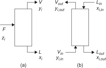
Figure 3.1 Input and output structure of separation involving (a) energy separating agent or membrane and (b) mass separating agent
and the component mass balance for species i is
where the stream flowrates (F, L, V) are either in mass or mole units, and the fractions (xi, yi, zi) are either mass fractions or mole fractions, respectively.
For a mass separating agent, such as extraction, as illustrated in Figure 3.1(b), wherein solute i is transferred from the liquid stream L to the vapor stream V or vice versa, the mass balances are
where, once again, if the flowrates are in mass units, the fractions are mass fractions, and if the flowrates are in mole units, the fractions are mole fractions.
The nomenclature used for these mass balances is in anticipation of liquid-vapor separations, hence the use of L and V. However, the mass balances are applicable to any separation modeled by either case in Figure 3.1.
3.1.2 Energy Balances
For the system illustrated in Figure 3.1(a), the overall energy balance is
where Q is the heat duty, in energy/mass or energy/mole, H is a vapor enthalpy, and h is a liquid enthalpy, both in energy/mass or energy/mole.
For the system illustrated in Figure 3.1(b), the energy balance is
For liquid-liquid separations such as extraction, all enthalpies are for liquids, and the energy balance is not usually needed, since little or no energy of solution is involved in transferring a solute between liquid phases, so the process is essentially isothermal. For some vapor-liquid separations, such as absorption and stripping, the energy balance may be involved, since dissolving a gas in a liquid is often accompanied by a heat of solution, which makes the process nonisothermal.
3.1.3 Equilibrium Relationships
For an equilibrium separation, it is assumed that the outlet streams are in equilibrium, or if the actual behavior is modeled as an approach to equilibrium, an equilibrium expression for each component must be solved along with the mass and energy balances. In effect, it is assumed that the phases are well mixed for a sufficient residence time to reach equilibrium. In general, the equilibrium relationship is of the form
where, for vapor-liquid separations
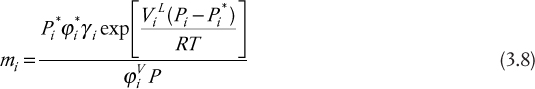
where Pi is the partial pressure of component i; ![]() is the vapor pressure of component i;
is the vapor pressure of component i; ![]() is the fugacity coefficient for component i at saturation; γi is the activity coefficient for component i; the exponential is known as the Poynting correction factor, with
is the fugacity coefficient for component i at saturation; γi is the activity coefficient for component i; the exponential is known as the Poynting correction factor, with ![]() being the liquid molar volume; and
being the liquid molar volume; and ![]() is the fugacity coefficient for component i in the vapor phase. The Poynting correction factor only deviates from unity at very high pressures. The fugacity coefficients only deviate from unity at high pressures, and the activity coefficient only deviates from unity for nonideal systems. Therefore, for ideal systems at low pressures, Equation (3.8) reduces to
is the fugacity coefficient for component i in the vapor phase. The Poynting correction factor only deviates from unity at very high pressures. The fugacity coefficients only deviate from unity at high pressures, and the activity coefficient only deviates from unity for nonideal systems. Therefore, for ideal systems at low pressures, Equation (3.8) reduces to

which is Raoult’s law. For liquid-liquid separations,

where the superscripts I and II refer to the two liquid phases. Usually, for liquid-liquid systems, experimental data are used, and if the data appear to be linear, a constant value for m can be determined. For gases dissolving, but not condensing, in liquids, m can be related to Henry’s law. In Henry’s law, the partial pressure in the vapor phase is related to the liquid mole fraction by pA = HAxA, where HA has pressure units, so m in Equation (3.7) becomes HA/P, where P is the total pressure.
3.1.4 Mass Transfer Relationships
3.1.4.1 Continuous Differential Model
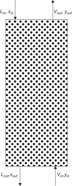
If the two phases being contacted in a separation are not well mixed, equilibrium is not reached between the phases. A model for this type of separation is similar to that for a countercurrent heat exchanger and is illustrated in Figure 3.2. In this development, it is assumed that there is one solute being transferred between phases, from the V phase to the L phase. The overall mass balances are Equations (3.3) and (3.4). Paralleling the heat transfer development in Chapter 2, the differential mass balance between two points S and S + ΔS is
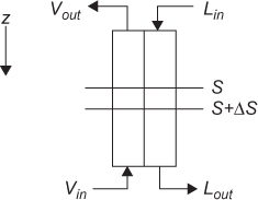
where Ny is the flux of solute in mass or moles/interface area/time and S is the interfacial (mass transfer) area/flow cross-sectional area, which is assumed to be zero at z = 0 and increase proportionally with the coordinate z. Equation (3.11) reduces to
A similar development under the assumption that transfer is from the L phase to the V phase gives
3.1.4.2 Two-Film Model
In order to apply Equation (3.12) or (3.13), a model for mass transfer between phases is needed. For transfer between immiscible phases (liquid-liquid or gas-liquid), the two-film model can be used. In this model, which is illustrated in Figure 3.3, there is a mass transfer resistance on each side of the interface described by a mass transfer coefficient, which is similar to a heat transfer coefficient. However, for mass transfer, there is a discontinuity in concentration at the film/film interface due to the difference in solubilities in the two phases, while for heat transfer the temperature is continuous across the films.

The flux on the V side for this case is (Treybal, 1980)

where cy is the total molar concentration, DABy is the diffusion coefficient of solute (A) in the V phase, δy is the film thickness in the V phase, yA is the mole fraction in the V phase, and yAi is the mole fraction in the V phase at the interface. Similarly, for the L phase,
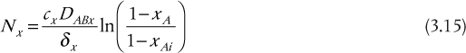
In this illustration, it is assumed that the direction of mass transfer is from the V phase to the L phase; however, the result is the same for transport in the opposite direction. At steady state, the flux from the V phase must be equal to the flux into the L phase. Equating Equations (3.14) and (3.15) yields

where Fy = (cyDABy/δy) and Fx = (cxDABx/δx). It is observed that Fx and Fy have the same units as N, moles/interfacial area/time. Since this model assumes a stagnant film, and in a real application there will also be convection, the parameters Fx and Fy are effectively mass transfer coefficients. The relationships for these mass transfer coefficients parallel those for heat transfer and are dependent on the actual flow geometry involved. Equation (3.16) can be used to calculate the values of yAi and xAi from the values far from the interface, based on the assumption that the interface is at equilibrium, so that yAi = mAxAi. It is important to understand that, when this model is used to describe a separation, equilibrium occurs only at the interface, whereas, in the well-mixed, equilibrium model described in Section 3.1.3, the phases are in equilibrium at all points in both phases, meaning that the outlet streams are in equilibrium. Equations (3.14), (3.15), and (3.16) can be simplified for special cases, such as dilute solutions, and these relationships are available (Treybal, 1980).
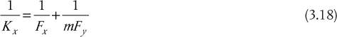
In the two-film model, the two mass transfer coefficients, Fx and Fy, can be combined into an overall mass transfer coefficient, just as in heat transfer. For an overall mass transfer coefficient based on the V phase, defined as Ky, this result is
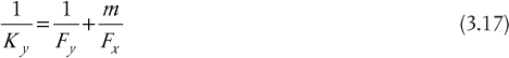
and the overall mass transfer coefficient based on the L phase, defined as Kx, is
3.1.4.3 Transfer Units
To determine the interfacial area required for a given separation, the differential equation obtained by using Equation (3.14) in Equation (3.12) or by using Equation (3.15) in Equation (3.13) must be solved. The former case is illustrated. The differential equation to be solved is
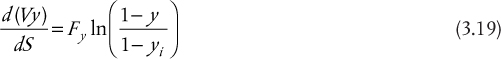
where the subscript A has been dropped. The result, presented here without derivation, is

In turbulent flow, the mass transfer coefficient is proportional to Re0.8 or a power close to 0.8 (just as in heat transfer), so the approximation that V/Fy is constant is often made. In this case, Equation (3.20) becomes

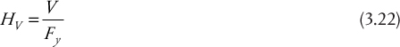
This form has the advantage of having one term (V/Fy) that is dependent on the flow geometry and one term (the integral) that is dependent only on the compositions of the phases for any flow geometry. These two terms are usually given the definitions “height of a transfer unit” (H) and “number of transfer units” (N), respectively. The use of the word height is based on a typical application to vertical, packed columns, although, the word length might be a better term. The height of a transfer unit is a measure of 1/separation efficiency, and the number of transfer units is a measure of the difficulty of the separation. The larger the height of a transfer unit, the less efficient the separation, and the larger the number of transfer units, the more difficult the separation. Therefore,
and
A parallel derivation is possible for the L phase, and the results are
and
In principle, the size (interfacial area) of a continuous differential separation unit calculated from either Equation (3.24) or Equation (3.27) is identical. This is similar to the area of a heat exchanger being identical for the two cases of the overall heat transfer coefficient based on the internal surface area (Ui) and the overall heat transfer coefficient based on the external surface area (Uo). The decision on which method to use is based on computational issues; however, it is generally true that the transfer unit expression for the phase with the limiting resistance is the better method to use.
It is also possible to define transfer units based on the overall mass transfer coefficients in Equations (3.17) and (3.18). All cases are presented in Table 3.2.

3.1.5 Rate Expressions
Some separations are based on differential rates of transport between components, so the rate of transport, not equilibrium, is used in conjunction with the mass and energy balances. The application that is treated here is membrane separations. The model for membrane transport is shown in Figure 3.4. An external resistance to mass transfer exists on either side of the membrane, which is characterized by a mass transfer coefficient (Fi). This model resembles heat transfer across a solid with external resistance, which was discussed for cylindrical coordinates in Chapter 2. The major difference is the concentration “jump” at the interface, while for the heat transfer case, the temperature is continuous across the interface. This is due to the different solute solubility in the membrane from that in the external phase. The steady-state flux (moles/interface area/time) of solute A across the membrane is
Assuming that the interfaces are at equilibrium, and using the equilibrium expressions CA1m = m1CA1i and CA2m = m2CA2i, Equation (3.28) can be rearranged into a series resistance form:
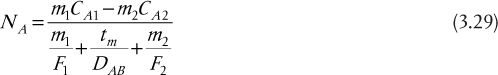
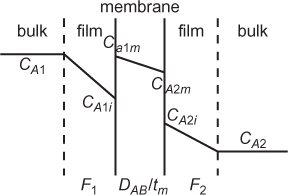
It is observed that the denominator of Equation (3.29) resembles the series resistance form in Equation (2.24). The difference, other than geometry, is the different solubilities of the solute in the membrane and in the two external phases. Analogous parameters are not present in the heat transfer form, because the temperature criterion for equilibrium at an interface is equal temperatures. For mass transfer, the criterion for equilibrium is the ratio of the solubilities in the two phases, mi, which is often called the partition coefficient.
In some cases, it is assumed that the external resistance is negligible, in which case Equation (3.29) reduces to
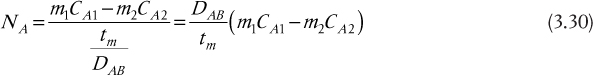
In the particular application discussed later in this chapter, the two external phases are gases, so it can be assumed that m1 = m2 = m, so Equation (3.30) further reduces to

where P is defined as the membrane permeability. (Note that some references define the permeability as P/tm.) In addition, for applications involving gas permeation, the concentrations are often expressed as partial pressures using the ideal gas law.
3.2 Illustrative Diagrams
3.2.1 TP-xy Diagrams
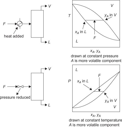
In traditional chemical processes, vapor-liquid separations are by far the most common. The simplest vapor-liquid separation is a partial condensation or partial vaporization. The discussion here is limited to binary mixtures with illustrations for ideal mixtures; however, the concepts apply to mixtures of any number of components and nonideal mixtures. In a partial condensation, a vapor mixture is brought into the two-phase region, and the vapor and liquid phases in equilibrium are at different mole fractions. Partial condensation can occur by either cooling and/or compressing a vapor mixture. Figure 3.5 denotes the equipment involved, and the separation is shown on a T-xy diagram. It is important to understand that either a heat exchanger or a compressor is needed to change the temperature or pressure, respectively. Quite often student problems and process simulators lump both pieces of equipment into one unit. Calculations can be performed this way, but the correspondence to actual equipment is lost. In Figure 3.5, the use of compression to form a two-phase mixture is shown only for illustrative purposes, since liquid droplets damage compressor rotors, meaning that this operation is not used. If compression was to be used, there would need to be cooling to facilitate condensation, since compression increases the temperature of the vapor. Figure 3.6 illustrates partial vaporizations, either by heating a liquid mixture into the two-phase region or by reducing the pressure of a liquid to form a vapor-liquid mixture. Once again, all relevant equipment is shown.

Quite often, all four of these operations are called flash separations. Technically, only the reduction in pressure is a “flash” separation, specifically a flash vaporization.
The equations used to solve any of these flash separations are the material balances, Equations (3.1) and (3.2); the energy balance, Equation (3.5); and the equilibrium expression, Equation (3.8). If Equations (3.1), (3.2), and (3.8) are combined, Equations (3.32) and (3.33) can be obtained.
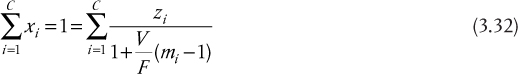

where the subscript i represents each component, and there are C components. In principle, either of these equations can be used to solve for one unknown, either V, temperature, or pressure (inside mi) if the other two are specified. Then, the mole fractions can be found. It is also possible, in principle, to solve for two of V, T, or P, with any two outlet parameters, including component mole fractions and fractional recoveries. However, since Equations (3.32) and (3.33) are not always monotonic, numerical methods can fail. Additionally, the difference between Equations (3.32) and (3.33) is always monotonic, so it is a better choice for a numerical solution.

Equation (3.34) is often called the Rachford-Rice equation (Wankat, 2017). The energy balance, Equation (3.5), is only used to calculate the heat duty on the heat exchanger used for the partial condensation.
In the production of cumene from propylene and benzene, the feed propylene contains propane, which does not react with the benzene. The reaction occurs in the vapor phase. The separation section of the process starts with a partial condensation of the unreacted benzene (present in excess to enhance selectivity) and cumene to remove the propane. For this example, it is assumed that all propylene in the feed reacts and that there are no unwanted by-products in the reactor effluent. The feed to the partial condenser contains 51 mol% benzene, 44 mol% cumene, and the remainder propane. Ideal behavior is assumed, and the Antoine coefficients are shown in Table E3.1 and are assumed to be valid over the temperature range of this problem.
If a partial condensation of 200 kmol/h occurs at 90°C and 1.75 bar, what are the flowrates and mole fractions of the streams leaving the flash drum?

Table E3.1 Antoine Coefficients for Example 3.1
Solution
Using Raoult’s law, the values of mi can be calculated from ![]() , where
, where ![]() is obtained from the Antoine coefficients in Table E3.1. Since zi are known, the only unknown in Equation (3.34) is V/F. Since there are only three terms in Equation (3.34), the result is a quadratic in V/F, although, in general, Equation (3.34) would be solved using an equation solver. The result is V/F = 0.0393, so V = 7.86 kmol/h, and L = 192.14 kmol/h. The mole fractions are obtained from
is obtained from the Antoine coefficients in Table E3.1. Since zi are known, the only unknown in Equation (3.34) is V/F. Since there are only three terms in Equation (3.34), the result is a quadratic in V/F, although, in general, Equation (3.34) would be solved using an equation solver. The result is V/F = 0.0393, so V = 7.86 kmol/h, and L = 192.14 kmol/h. The mole fractions are obtained from
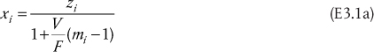
which are the individual terms in Equations (3.32) and (3.33), respectively, and m is given by Equation (3.9). The results are

If V/F were known, either the temperature or pressure could be obtained using the same method, solving for one unknown.
In the process in Example 3.1, the vapor stream contains too much benzene, a valuable reactant. The feed flowrate of benzene is 102 kmol/h, while the flowrate of benzene in the liquid phase is (192.14 kmol/h)(0.515) = 98.95 kmol/h, which is about 97% recovery of benzene in the liquid and a loss of about 3 kmol/h of benzene, which has a value of several million dollars/year. Under what operating conditions would 99% recovery of benzene in the liquid stream be possible?
Solution
In this case, V/F, T, and P are initially unknown. As in Example 3.1, two specifications are needed. One is the desired fractional recovery. The other is either T or P. V/F cannot be specified, because the material balance is determined by the fractional recovery specification. Therefore, if T is specified, the required pressure can be calculated, and vice versa.
The fractional recovery specification must be used to determine V/F. This specification is
which means that LxB = 100.98, so VyB = 1.02, since there are 102 kmol/h of benzene in the feed. Taking the ratio of these terms,
so

and rearrangement yields
If Equation (E3.3d) is inserted into Equation (3.34), then if the pressure is known, temperature is the only unknown, and vice versa. Therefore, there are actually an infinite number of temperature-pressure combinations that solve the problem. For this exercise, the pressure will be determined at 90°C, the original temperature in Example 3.1, and the temperature will be determined at 1.75 atm, the original pressure in Example 3.1. An equation solver is used, and at 90°C, the pressure is 2.14 atm, and at 1.75 atm, the temperature is 81.2°C. The mole fractions in each phase could then be calculated just as in Example 3.1.
Examples 3.1 and 3.2 illustrate that, without consideration of energy requirements, Equation (3.34) can be used to solve for a single unknown with two specifications. The energy balance, Equation (3.5), can be used the get the heat duty. Problems that couple the energy balance with Equation (3.33) are also possible.
It is observed from the T-xy diagrams that the vapor phase is enriched in the more volatile component, while the liquid phase is enriched in the less volatile component. The horizontal line connecting the vapor and liquid phases in equilibrium is called a tie line. Any mixture brought to a point in the two-phase region separates into two phases connected by the tie line. It is further observed that neither phase is very pure in the enriched component. Now, suppose that the feed is vapor that is partially condensed, and the vapor phase, V1, is partially condensed again, as illustrated in Figure 3.7, and the process is repeated several times. It is observed that the more volatile component can asymptotically approach purity. Similarly, Figure 3.7 also illustrates that the less volatile component can asymptotically approach purity by partially vaporizing the liquid phase. Each heat exchanger/drum combination is called a stage, and these are called equilibrium stages, because it is assumed that the two phases leaving the stage are in equilibrium. This sequence appears promising; however, as shown Figure 3.7, there are a significant number of waste streams, since only the top or bottom stream is the desired product. Furthermore, a significant number of heat exchangers is required. Suppose the top “waste” stream is recycled to the second-from-the-top stage. It can provide the necessary heat sink in place of one partial condenser. This is illustrated in Figure 3.8. Similarly, if the bottom waste stream is recycled from the second-from-the bottom stage, it can provide the energy for one partial vaporization. This is also illustrated in Figure 3.8. Every waste stream can be returned to the adjacent stage, and Figure 3.9 illustrates the entire process, and it is observed that there is one feed stream and two exit streams, both of which can be very pure in one of the components. Heat is added only at the bottom and energy is removed only at the top. This is how distillation works, although as will be seen later, the actual equipment is more compact.


It is important to realize that while the T-xy diagram provides a mental picture of how distillation works, it is not used for calculations, though it was before high-speed computing. The calculations are done exactly how the diagrams suggest, using a series of mass and energy balances combined with equilibrium expressions from stage to stage, as shown in Section 3.1.
If it is understood that energy is required to “unmix” components, which lowers the system entropy (since mixing is spontaneous), it is no surprise that energy must also be rejected to the surroundings. Overall, energy input is required to unmix the components, but energy must also be rejected to the surroundings, just as in a power cycle.
3.2.2 McCabe-Thiele Diagram
The McCabe-Thiele diagram is a graphical representation of distillation, and it can also be used to represent separations using mass separating agents. It is valid only for certain systems subject to certain assumptions. While current computational power makes the McCabe-Thiele diagram somewhat obsolete, an understanding of the diagram provides conceptual insights that apply to all types of distillation operations and to all types of separations using mass separating agents.
3.2.2.1 Distillation
The McCabe-Thiele diagram can be used to represent distillation using either tray columns or packed columns.
Tray Columns
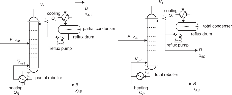
A schematic of a tray distillation column is shown in Figure 3.10(a), along with a detailed sketch of the internals of a distillation column in Figure 3.10(b). It is a tower with trays containing holes, sometimes with caps or similar devices on top of the holes. A level of liquid is present on each tray, and gas bubbles up through the tray from the tray below. Each tray behaves like a flash operation. The feeds to each tray, one from the top and the other from the bottom, are at different temperatures so that the liquid and vapor on the tray are assumed to come to equilibrium. Since the vapor bubbles through the holes in the tray, the bubble motion is assumed to create a well-mixed condition, so that the exit streams from the tray are at the same conditions as the vapor and liquid on the tray.

Figure 3.10 (a) Schematic of distillation column, (b) internals of distillation column (b from Couper et al. [2012])
The material and energy balances, as described by Equations (3.3), (3.4), and (3.6), are written for every tray. An alternative method is to write these balances from the top to each tray above the feed and the bottom to each tray below the feed. One of these sets of balances, along with balances on the condenser, reboiler, and feed tray, are solved simultaneously. Therefore, the number of trays must be known, so that all balances can be written. This means that the outlet conditions can be predicted for a fixed number of trays, feed location, reflux ratio (L0/D in Figure 3.10[a]), and feed conditions, which is a simulation, not a design. To design a column this way requires iterations, until the number of trays, reflux ratio, and feed location provide the desired outlet conditions. This is why process simulators require that the number of trays and feed location be provided for a rigorous distillation calculation.
There is a simplification that allows a graphical method to design a distillation column. It only works for binary distillations under certain circumstances. However, a complete understanding of this method provides a complete understanding of the operation of a distillation column. This is the approach taken here.
The assumption that simplifies binary distillation calculations is called constant molar overflow (also called constant molal overflow). The assumptions of constant molar overflow are
• Molar heat of vaporization (λ) is the same for each component.
• Column is adiabatic.
• Sensible heat is small compared to latent heat (CpΔT < < λ).
As a consequence, the moles of vapor condensing on a tray equal the moles of liquid vaporizing on the tray. Therefore, the molar flowrates of liquid and vapor do not change from tray to tray in a given section of the column (a section is either above the feed or below the feed). Additionally, there is no need for an energy balance on any tray, because the energy need for vaporization equals the energy given up by condensation, and since no heat is lost, the heats of vaporization are identical, and they are much larger than any temperature changes between adjacent trays.
Material balances written from the top of the column to a tray (j) above the feed, as illustrated in the top portion of Figure 3.11, are

where the assumption of constant molar flowrates on every tray is used, so that L and V are constant and not indexed by tray number. (Note that trays are numbered from top to bottom.) Equation (3.36) is written on the more volatile component, A. Equations (3.35) and (3.36) can be rearranged to

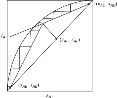
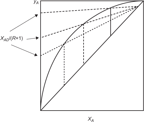
where R = L/D. Equation (3.37) is now written as
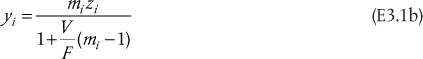
where the subscript for the tray number has been dropped, since the equation is the same for a balance written from the top of the column to any tray. Equation (3.38) is the equation of a straight line with slope L/V and intercept xAD/(R + 1). While it is possible to plot this line if L/V is known, an easier method is to observe that when yA = xA, xA = xAD. Therefore, two points are known, the intercept and (xAD, xAD). When this line is plotted on an equilibrium diagram, the line labeled 1 in Figure 3.12 is obtained. On Figure 3.12, the curve represents the vapor-liquid equilibrium, which can be obtained from the endpoints of the tie lines on a T-xy diagram such as shown in Figure 3.9. These data can be predicted from Raoult’s law or, in the most general case, Equation (3.8). The diagonal line is just a plot of yA = xA.
A similar analysis can be done by writing a material balance from the bottom of the column to any tray below the feed. The situation is illustrated in the lower portion of Figure 3.11. The equations are
where the overbar indicates molar flowrates below the feed. Equations (3.39) and (3.40) can be rearranged to yield, with removal of the index subscript

Equation (3.41) is the equation of a straight line with slope ![]() and intercept
and intercept ![]() . If yA = xA, xA = xAB. Therefore, two points are known, the intercept and (xAB, xAB). This line is plotted on Figure 3.12 and labeled 2. It is observed that the intercept is negative because the slope
. If yA = xA, xA = xAB. Therefore, two points are known, the intercept and (xAB, xAB). This line is plotted on Figure 3.12 and labeled 2. It is observed that the intercept is negative because the slope ![]() .
.
The upper section of a distillation column, above the feed, is called the enriching section or the rectification section. The lower section, below the feed, is called the stripping section. The feed tray is the boundary between these two sections. In general, liquid in the feed goes down and vapor goes up; however, what exactly happens on the feed tray depends on whether the feed is saturated liquid, saturated vapor, a vapor-liquid mixture, superheated vapor, or subcooled liquid. It is important to understand that these terms are defined relative to the conditions on the feed tray. For example, if the feed is saturated liquid at 30°C, but the tray temperature is 50°C, then the feed is considered subcooled.
To complete the column model, the top and bottom sections must match at the feed. Figure 3.13 illustrates the feed tray.
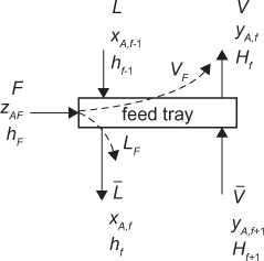
The material and energy balances on the feed tray are
where the subscript f indicates the feed tray number, uppercase H indicates vapor enthalpy, lowercase h indicates liquid enthalpy, and hF is the enthalpy of the feed regardless of its phase. If the feed stage is assumed to be at equilibrium, then the vapor and liquid enthalpies are for saturated conditions. From the constant molar overflow assumption, the enthalpies of each phase are constant across the trays, so, rearranging Equations (3.42) and (3.43), while dropping the subscripts involving f, yields an equation for the quality of the feed, q, defined as the fraction of the feed in the saturated liquid state (as opposed to the quality of steam, which is defined as the fraction of vapor in the steam):
If the feed is saturated liquid, q = 1, so the liquid flowrate below the feed is equal to the liquid flowrate above the feed plus the feed flowrate. The vapor flowrates above and below the feed are identical.
If the feed is saturated vapor, q = 0, so the vapor flowrate above the feed is equal to the vapor flowrate below the feed plus the feed flowrate. The liquid flowrates above and below the feed are identical.
If the feed is a vapor-liquid mixture, 0 < q < 1, so the liquid flowrate below the feed is equal to the liquid flowrate above the feed plus the liquid flowrate in the feed, LF. The vapor flowrate above the feed is the vapor flowrate below the feed plus the vapor flowrate in the feed, VF. Simply put, saturated liquid goes down, and saturated vapor goes up.
Subcooled liquid and superheated vapor are not as simple. For a subcooled feed, the feed enthalpy, hF, is less than the saturated liquid enthalpy, h. Therefore, q > 1, which means that the liquid flowrate below the feed is greater than the liquid flowrate above the feed plus the feed flowrate. How is this possible? Since the denominator of the enthalpy expression in Equation (3.44) is the heat of vaporization (also called latent heat), more energy is required to bring the feed to equilibrium on the feed tray than can be supplied by the condensing vapor. In order for the subcooled liquid in the feed to come to the equilibrium conditions on the feed tray, enthalpy is required. This enthalpy comes from condensing some of the saturated vapor. Therefore, the liquid flowrate below the feed increases by more than the feed flowrate. Additionally, the vapor flowrate above the feed is lower than the vapor flowrate below the feed, since some vapor condenses on the feed tray.
A similar explanation exists for superheated vapor. Since hF > H, q < 0. The superheated vapor must give up enthalpy to become saturated on the tray, which is obtained by vaporizing some liquid on the tray. Therefore, vapor flowrate increases above the feed tray and the liquid flowrate decreases below the feed tray.
It can now be seen that
where the subscript F indicates feed. Adding Equations (3.36) and (3.40) with Equation (3.45), and then applying the overall more volatile component balance
yields

Equation (3.47) is the equation of a line with slope q/(q – 1) and is called the q-line. If yA = xA, it can be seen that one point on the line is (zAF, zAF). Since the balances from the top and bottom sections were combined to give Equation (3.47), the top section, the bottom section, and the q-line must all intersect. This is illustrated in Figure 3.14 for a vapor-liquid mixed feed. Since the slope of the q-line is q/(q – 1), it can be seen that there are five possible q-lines, representing the different possible feeds, which are illustrated in Figure 3.15. Table 3.3 summarizes these results.

Table 3.3 Mole Balances, Feed Condition, and Slope of q-line for Different Distillation Column Feed Conditions
The ideal feed location is where the feed stream and the tray conditions match, which means matching composition, temperature, and pressure. Of course, the feed stream must be at a slightly higher pressure than the feed tray to allow flow into the column. So, a liquid feed would be brought close to saturation before entering the column. If the vapor effluent from a reactor were to be fed directly to a column, it would be cooled close to saturation. Two-phase feeds are also possible. If the column diameters above and below the feed are different enough to make it impossible to have a column of uniform diameter, the feed conditions could be adjusted to equalize the top and bottom diameters. Therefore, in extreme situations, subcooled liquid or superheated vapor feeds might be desirable.
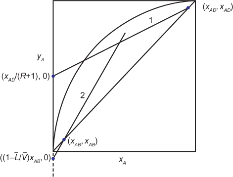
The McCabe-Thiele method can be used to determine the number of equilibrium stages needed for a separation. If the desired top and bottom compositions are specified (or alternatively, fractional recoveries) and a reflux ratio chosen, the upper operating line can be drawn, and the lower operating line is drawn from the intersection of the upper operating line and the q-line. Then, as is illustrated in Figure 3.16, the number of stages can be stepped off starting at the top with alternating horizontal lines and vertical lines. A horizontal line to the equilibrium curve is the solution to the equilibrium on a tray, and the vertical line to the operating line is the material balance on that tray (or from the top to any tray above the feed, or from the bottom to any tray below the feed). Each step is an equilibrium stage, so the total number of steps is the number of equilibrium stages required. It is observed that the vertical lines change from the upper operating line to the lower operating line when the step straddles the intersection of the q-line and the operating lines. This represents the optimum feed location that minimizes the number of stages. In Figure 3.16, the feed is on Stage 4 (always count from the top), and there are >7 stages. In the design phase, fractional stages can exist. Before the column is constructed, the extra stage would be added, and it would be planned to operate at a slightly different reflux ratio to make the bottom step intersect the point (xAB, xAB).
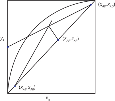
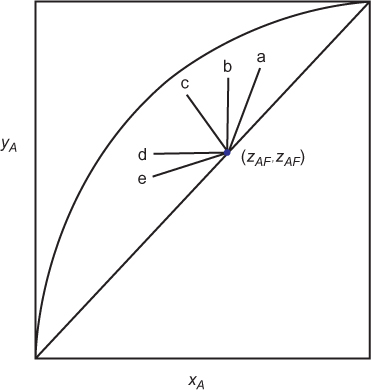
Figure 3.15 Different feed (q) lines for different feeds: (a) subcooled liquid, (b) saturated liquid, (c) vapor-liquid mixture, (d) saturated vapor, (e) superheated vapor
A total condenser and a total reboiler are not equilibrium stages, since saturated vapor at the dew point is condensed to saturated liquid at the bubble point (total condenser), or vice versa (total reboiler). A partial condenser and a partial reboiler are equilibrium stages, since the condensation or vaporization is “partial” and there are equilibrium phases in equilibrium, just as in a flash operation. Partial condensers are used if a vapor product is needed or if there are noncondensable components. In appropriate applications, there can be a partial vapor-liquid condenser, in which noncondensables are removed as vapor, but a condensable, desired product is removed as a liquid. All of these configurations are illustrated in Figure 3.17. There is also a reflux drum present with a controlled liquid level to smooth out fluctuations. The reflux pump is necessary, because in an actual process, the condenser, reflux drum, and reflux pump are likely to be located close to the ground, so the pump provides pressure to overcome the head to return the reflux to the top of the column.
Despite the limitations of the McCabe-Thiele method, a complete understanding of the graphical representations provides an understanding of distillation, including distillation with more than two components and distillation systems for which the constant molar overflow assumption is not valid.
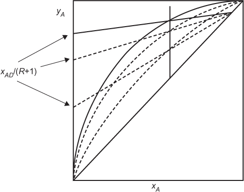
In a chemical plant, about the only variable that can be adjusted is a flowrate. In a distillation column, the flowrate that is adjusted is the reflux stream, which is typically described in terms of the reflux ratio, L/D. Figure 3.18 illustrates four different reflux ratios for a saturated liquid feed; however, the discussion that follows applies to any feed condition. Only the upper section of the column is shown. In Figure 3.18(a), the upper operating line intersects the equilibrium line and the q-line at the same point. If stages are stepped off, the intersection point is never reached. This is the minimum reflux ratio. The operating line in Figure 3.18(a) represents the minimum reflux ratio, which requires an infinite number of stages. However, if the reflux ratio is increased slightly, which lowers the y-intercept, as illustrated in Figure 3.18(b), a finite number of stages can be counted. As the reflux ratio increases, the intercept decreases, the steps get larger, and fewer equilibrium stages are needed. When the intercept equals zero, the reflux ratio is infinite, called total reflux, which is illustrated in Figure 3.18(d). At total reflux, there are no product streams and no feed. This is an operational limit, which is used to start up a distillation column and bring it to steady state. Therefore, the McCabe-Thiele diagram illustrates a key concept in distillation, that increasing the reflux ratio reduces the number of equilibrium stages required to obtain the same product specifications. A concept introduced in Chapter 1 is that just about the only way to adjust anything in a chemical process is to open or close a valve. In distillation, there would be valves included to adjust the ratio of L0/D in Figure 3.17. This is how the reflux ratio is adjusted.

Figure 3.18 Effect of increasing reflux ratio on number of stages. Part (a) reflects minimum reflux, and Part (d) reflects total reflux.
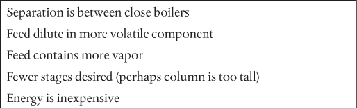
As the boiling points of the two components being distilled become closer, the equilibrium curve moves toward the diagonal line, since the equilibrium liquid and vapor mole fractions become closer together. Figure 3.19 illustrates that the minimum reflux ratio must be higher for a separation involving closer boilers, since, for the same feed, the y-intercept is smaller. Therefore, the actual reflux ratio must also increase for closer boilers.
The feed composition also affects the reflux ratio. The q-line moves to the left if the feed is dilute in the more volatile component. Figure 3.20 illustrates how a more dilute feed in the more volatile component requires a larger reflux ratio. Once again, only the minimum reflux ratio is shown.
The feed condition also affects the required reflux ratio, as is illustrated in Figure 3.21 for the minimum reflux ratio for each feed condition. Subcooled liquid requires the lowest reflux ratio, while superheated vapor requires the highest reflux ratio.

While it is difficult to illustrate, as the desired distillate mole fraction approaches 1.0 for a fixed number of stages, the slope of the upper operating line increases, so the intercept decreases, which means that a larger reflux ratio is needed.
As the reflux ratio increases, all of the internal flowrates increase. As will be seen later, there is an associated increase in column diameter, but, as already stated, fewer equilibrium stages are required. However, as the internal flowrates increase, the amount of liquid that must be condensed and the amount of vapor that must be reboiled both increase, thereby increasing the heat duties of the condenser and reboiler. For a total condenser, the energy balances is
Since hL = hD, because the enthalpy does not change when a stream splits, and since V = L + D, Equation (3.48) becomes

which is how the condenser heat duty can be calculated. The approximation in the last equality in Equation (3.49) includes the assumptions of ideal gas behavior and ideal liquid solutions. If these conditions are not valid, a standard thermodynamic method for calculating the enthalpies of the vapor and liquid mixtures would be used. Equation (3.49) also shows that as the flowrate of the vapor stream increases, the condenser heat duty increases. For a given separation, with fixed feed and outlet flowrates, the value of V increases as reflux ratio increases; therefore, the condenser heat duty also increases.
A similar development for the reboiler yields

where, once again, it is seen that as the internal flowrates increase, the reboiler heat duty also increases.
The energy balances clearly show that as the reflux ratio increases, the heat duties increase, which means that the operating cost (virtually all heating and cooling utilities) of a distillation column increases.
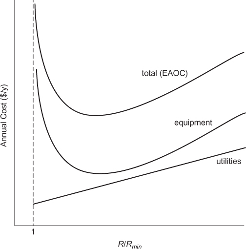
Table 3.4 summarizes the reasons for needing a high reflux ratio. Table 3.5 summarizes the effect of increasing the reflux ratio. Figure 3.22 illustrates the economics of a distillation column, and it is noted that Figure 3.22 is an illustration and not drawn to scale. As the reflux ratio increases, the number of trays decreases, so the cost of the column decreases. As the reflux ratio increases further, the diameter increases, so the cost of the column increases. As the reflux ratio increases, the cost of energy (utilities) increases, and the cost of the condenser and reboiler also increases. If the equipment cost is put on the same basis as the operating cost (utilities), which is done by assuming that the equipment cost is equivalent to a loan with periodic payments, the resulting curve suggests that there is an optimum reflux ratio. EAOC stands for Equivalent Annual Operating Cost, which is the sum of the actual operating costs (utilities) and the periodic payment on the initial equipment cost. The location of this optimum value for R/Rmin is a strong function of the cost of energy. In the mid-20th century, when energy was inexpensive, optimum values in the 1.5 to 1.8 range were recommended. In the latter part of the 20th century, when energy prices increased, optimum values in the 1.2 to 1.5 range were recommended. In the early 21st century, energy prices have fluctuated significantly, so it is important to remember that the optimum value changes with energy prices.

Packed Columns
A schematic of a packed column is shown in Figure 3.23. The concept is that liquid coats the packing, providing vapor-liquid surface area for mass transfer, similar to the vapor-liquid interface created by bubbles in tray columns. The packing can be random or structured. Random packing consists of small objects, for which there are a multitude of shapes, and the details are discussed later. These objects are randomly placed in a large, empty column. In contrast, structured packing consists of sections with a solid/void structure that are layered into the column. The key parameter is the interfacial area, introduced in Section 3.1.4. Separations in packed columns are continuous differential separations rather than staged separations. In continuous differential separations, equilibrium is assumed to exist at the vapor-liquid interface. The height of the column becomes the design parameter, as opposed to the number of stages.
The height can be obtained from the interfacial area/cross-sectional area, S, by defining a mass transfer area, a, that is specific to each type of packing, having units of mass transfer area/packed volume. The packed volume includes the void fraction, which is specific to the packing dimensions and shape. Therefore,
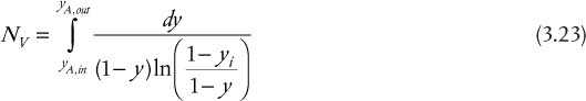
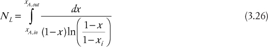
where Z is the height of the column.
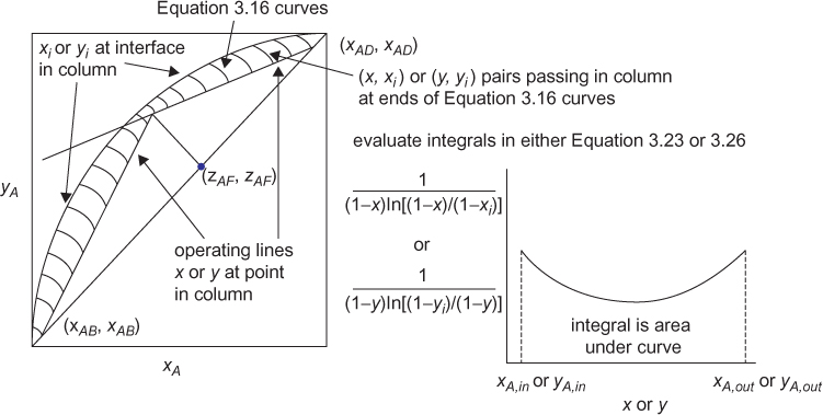
If the mass transfer area, a, of a packing is known, then the height, Z, can be calculated from S in Equation (3.51). Manufacturers provide specifications on packings, and there is an extensive literature available for some of the most common packing materials. The interfacial area/cross-sectional area, S, can be calculated from the height and number of transfer units. For this explanation, vapor transfer units and heights are used, as described in Equation (3.24). The height of a transfer unit HV = V/Fy in Equation (3.22) can be calculated if the internal flowrates are known, since there are correlations available for the mass transfer coefficient Fy. The question is how to evaluate the integral for the number of transfer units, NV, in Equation (3.23). For this type of analysis, a McCabe-Thiele diagram is drawn, just as for staged separations; however, stages are not stepped off. The integral must be evaluated separately above the feed and below the feed, so one limit on each integral is the feed composition. As the values of mole fraction are varied between the feed and the distillate (top of column) and the feed and bottom (bottom of column), Equation (3.16) can be used with the material balance line (operating line) to determine pairs of corresponding values of y and yi. The graphical representation of the simultaneous solution for this problem is illustrated in Figure 3.24. Consistent with the two-film model in Figure 3.3, points on the operating line represent passing stream mole fractions at every point in the column. Similarly, points on the equilibrium curve represent the interface composition, assumed to be in equilibrium, at every point in the column. This set of pairs of (x, y) and (xi, yi) allows the integral in Equation (3.23) to be evaluated numerically. The total height of the column is the sum of the heights of the upper and lower sections, and the feed height is clearly defined. An important concept to understand is that Figure 3.24 clearly shows that equilibrium occurs at the interface at every location in the column, but that the equilibrium values are different at different values of the column height.
3.2.2.2 Mass Separating Agents
The McCabe-Thiele method can also be used for separations with mass separating agents. There are some differences. In binary distillation, both components are volatile. On any stage, the more volatile component is transferred from the liquid phase to the vapor phase, while the less volatile component is transferred from the vapor phase to the liquid phase. For mass separating agents, the idealized situation is that a solute is transferred from one phase to a different phase, where both solvents are immiscible. The phase pairs can be gas-liquid (absorption and stripping), liquid-liquid (extraction), solid-liquid (leaching, washing, adsorption), or solid-gas (adsorption). (The difference between gas [e.g., air] and vapor is that the former does not condense at or near typical operating conditions, whereas the latter can condense at typical operating conditions.)
The rigorous method is to solve Equations (3.3) and (3.4) simultaneously for every stage. For gas-liquid systems (absorption and stripping), energy balances might also be needed, since dissolving a gas into a liquid (absorption), HCl into water, for example, produces a heat of solution and a noticeable temperature change. For separations such as extraction and adsorption from a liquid, heat effects are usually negligible. If there are negligible heat effects and if the solvents are completely immiscible, the McCabe-Thiele method is applicable. If there is only one solute and two immiscible solvents and if the mole fractions are small enough, the total flowrates are approximately constant. Under these circumstances, Equation (3.4) can be rewritten as
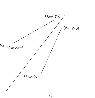
where the subscript i has been dropped, since there is only one solute. This is the equation of a straight line on a plot of y versus x with slope L/V connecting the points representing the inlet and outlet mole fractions. This is illustrated in Figure 3.25, assuming countercurrent operation, with an arbitrary equilibrium curve. For multistage separations, countercurrent is the norm. If the two phases flow in the same direction, called cocurrent separations, once equilibrium is attained in the first stage, all subsequent stages would be useless, since the feed to those subsequent stages would already be at equilibrium.
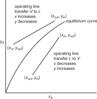
Another difference between distillation and mass separating agents is that the operating line can be on either side of the equilibrium curve. As illustrated in Figure 3.25, if the solute transfers from the V phase to the L phase, xout > xin, and yout < yin, since each point on the operating line represents streams passing in the opposite direction. If the solute transfers from the L phase to the V phase, xin > xout, and yin < yout. If there are multiple stages, Equation (3.52) can be rewritten from one end of the cascade of stages to any intermediate stage
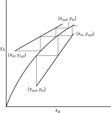
which is the equation of the operating line for the separation. Once this operating line is known, the stages can be stepped off, as illustrated in Figure 3.26.
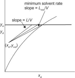
Consider a separation involving transfer from the V phase to the L phase. The inlet mole fractions, yin and xin, would be known along with the inlet flowrate of the V phase, V. The purpose of the separation is to remove solute from the V phase, so the inlet mole fraction would be known. The inlet mole fraction of the L phase would presumably be known and be very small, if not zero. There would probably be a target amount of solute to be removed or a target outlet mole fraction, so yout would also be known. Figure 3.27 shows that the flowrate L can have multiple values for a fixed value of V, but as L gets smaller, resulting in a smaller slope, the operating line gets closer to the equilibrium curve, resulting in more steps, meaning more stages are needed. This is analogous to the trade-off between reflux ratio and number of stages in distillation. The destination solvent rate replaces the reflux ratio. There is also a minimum solvent rate, which is determined either by the intersection of yin with the equilibrium curve or by a tangent, depending on the curvature of the equilibrium curve.
For continuous differential separations, the operating line and equilibrium curves are similar to those in staged separations, since there is an equilibrium relationship and since the operating line represents the tray-to-tray mass balances. The method described in Section 3.2.2.1 would be used to evaluate the integral for the number of transfer units.
3.2.3 Dilute Solutions—The Kremser and Colburn Methods
Under the following conditions, an analytical solution can be found for countercurrent separations. The assumptions are
• Dilute solutions
• Total stream flowrates remain constant
• Equilibrium relationship is linear
• Isothermal operation
• No energy associated with transfer between phases
The results are presented without derivation. The result for transfer from the V phase to the L phase for staged separations is called the Kremser method (Kremser, 1930; Souders and Brown, 1932) and is

where A = L/mV and is called the absorption factor (because this method is traditionally applied to gas absorption into a liquid, but it is valid for any separation that is consistent with the assumptions), N is the number of stages, and m is the partition coefficient from the equilibrium expression y = mx. Equation (3.54) can be written explicitly for N as
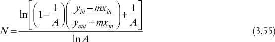
There is no explicit relationship for A. For transfer from the L phase to the V phase, the equivalent relationship is shown in Table 3.6. When A = 1, Equations (3.54) and (3.55) are indeterminate. The results for such a case, obtained from application of L’Hôpital’s rule, are also presented in Table 3.6.
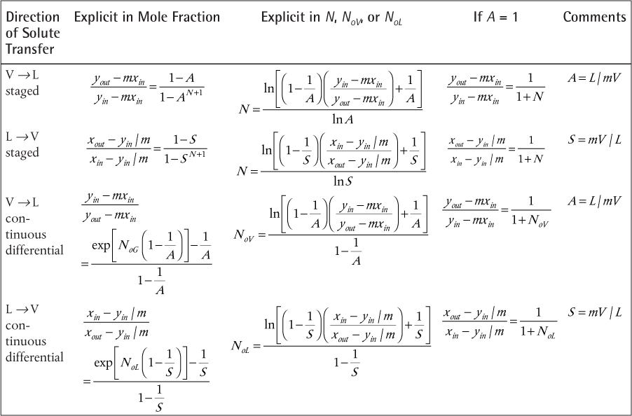
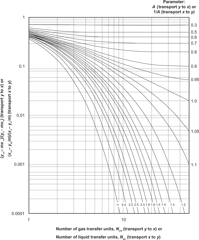
For continuous differential separations with transfer from the V phase to the L phase, the relationships are attributed to Colburn (1939) and are
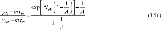
and
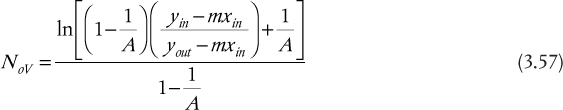
where NoV is defined in Table 3.2.
Table 3.6 summarizes the relationships presented for transfer from the V phase to the L phase and also presents the relationships for transfer from the L phase to the V phase. In the latter case, S is the stripping factor, which is the inverse of the absorption factor.
The Kremser and Colburn results are often presented in graphical form, and they are shown in Figures 3.28 and 3.29, respectively. Although it is easy to solve the equations, even for A, similar to the McCabe-Thiele method for distillation, a thorough understanding of these graphs provides a full conceptual understanding of separations involving mass separating agents.
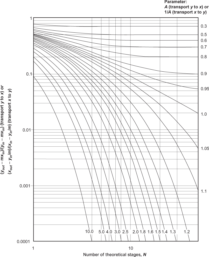
Consider a separation with transfer from V to L. It is desired to remove solute from the V phase such that yout/yin = 0.1 using a pure solvent, so xin = 0. Point a on Figure 3.30, which is a blown-up portion of Figure 3.28, shows one possible solution to the problem, N ≈ 5.0 and A = 1.2. Moving along the horizontal line in either direction shows that the same separation can be accomplished by increasing N and decreasing A, and vice versa. Since A ∝ L, this illustrates the trade-off between the number of stages and the solvent flowrate. If it is desired to improve the separation such that yout/yin = 0.005, there are two possible methods. One is to increase N at constant A, adding more stages, which makes sense. This is illustrated by following the A = 1.2 line down to Point b on Figure 3.30. Another possibility is to increase A at constant N, which is illustrated by the vertical line down to Point c on Figure 3.30. There are two ways to increase A, increase the solvent flowrate L, which should make sense. Another method is to decrease m. Since y = mx at equilibrium, decreasing m decreases the ratio y/x, which means that the L-phase mole fraction at equilibrium increases and/or the V-phase mole fraction decreases at equilibrium, favoring the L-phase. For the specific application of gas absorption, an expression for m might be m = P*/P. If the pressure increases, m decreases, which makes sense since increasing the pressure favors the liquid phase. If the temperature decreases, P* decreases, so m decreases, which makes sense since decreasing the temperature favors the liquid phase. For a given target separation, if a certain A value is needed, an unfavorable m value, which is a large value for absorption, can be overcome by increasing L as much as needed. While this works in principle, there could be operability issues.

To generalize, even though all separations involving mass separating agents do not follow the assumptions in the Kremser or Colburn methods, a thorough understanding of those graphs provides a thorough understanding of the trends in separations involving mass separating agents. To reiterate what is illustrated in Figure 3.30, Point a shows a target separation, as defined by a value on the y-axis (which is the same y-axis as in Figures 3.28 and 3.29). It is being accomplished with a certain number of stages (or transfer units) at a certain A (or S) value. The same level of separation, defined by the same value of the y-axis, can be achieved with a lower A value and more stages (Point d) and a larger A value and fewer stages (Point e). This illustrates a trade-off between the absorption (stripping) factor and the number of stages (transfer units). Within the absorption (stripping) factor, for the purposes of this example, it is assumed that the equilibrium constant cannot be changed and that the value of L (V) is fixed by upstream demands (meaning that the flowrate of material that must be processed in the separator is fixed). A higher A (S) value corresponds to a higher liquid flowrate (vapor flowrate). This means that the trade-off between absorption (stripping) factor and the number of stages (transfer units) is actually a trade-off between liquid (vapor) flowrate and the number of stages (transfer units). Since A (S) is the key parameter, this also demonstrates how to overcome an unfavorable equilibrium condition. For transfer from V to L, it would be desirable for m to be less than unity, meaning the mole fraction in the liquid phase is always less than that in the vapor phase. This means that the equilibrium favors the liquid phase. However, if m is greater than unity, which alone reduces the value of A (S), the value of A (S), the unfavorable equilibrium can be offset by increasing the value of the destination solvent, L (V). There are equipment limitations to the relative flowrates of the two phases that are dependent of the specific phases involved, and these will be discussed later in the chapter. Finally, at a constant number of stages (transfer units), if A (S) is increased, the value of the y-axis decreases, which means a better separation. This is illustrated by the vertical line through Points a and c in Figure 3.30.
If A < 1, where A is the absorption factor, L/(mV), there is a limiting behavior. It can be seen that for A < 1, increasing the number of stages does not improve the separation beyond an asymptotic limit. Normally, it would be expected that increasing the number of stages would improve the separation, but this is only true for A ≥ 1. The reason can be understood by looking at the McCabe-Thiele diagrams shown in Figure 3.31. If the equilibrium line is defined by y = mx, and the slope of the operating line is L/V, as shown in Section 3.2.2, then, if A < 1, L/V < m, so the operating line approaches the equilibrium line at the bottom of the column (see also Figure 3.25), which is the most concentrated part of the column. Therefore, since the solution is approaching saturation at the concentrated portion of the column, where solvent capacity is needed most, the ability to transfer solute is limited, causing the observed asymptote. If A ≥ 1, L/V > m, equilibrium is approached at the less concentrated portion of the column. For transfer in the opposite direction, while the operating line is below the equilibrium line, the argument is exactly the same.
For continuous differential separations, the discussion just presented is identical, except that the number of transfer units replaces the number of stages. Once again, it is important to remember that the number of transfer units is not numerically equal to a number of stages. However, as the number of transfer units increases, the required interfacial area increases (Equation [3.24]). For a gas-liquid separation, this means that the height of the packed column increases. Similarly, as the number of trays increases, the height of a tray column increases.
For other separations, such as liquid-liquid extraction, if the equilibrium is linear and the solutions dilute, the Kremser and Colburn methods can be used, and all of the same trends are true. Quite often, liquid-liquid equilibrium obtained experimentally is expressed in terms of mass fraction, so the flowrates become mass flowrates. In most textbooks, the letters used to represent these flowrates are different to conform with chemical engineering jargon. The output stream from the feed stream (F) is called the raffinate (R). The destination solvent input stream is denoted S, and its output stream is called the extract (E). To avoid confusion of letters, an alternative method is to retain the symbols L and V and use L for the heavier (more dense) phase (often water) and V for the lighter (less dense) phase (usually organic). In reality, as long as the equilibrium expression is written correctly, the choice of symbols used is irrelevant.
Consider a gas-liquid separation in which acetone in air is absorbed into water to purify the exhaust air. The equilibrium is described by Raoult’s law, and the vapor pressure is given by
An absorber is to be designed to treat 100 kmol/h of air containing a mole fraction of 0.05 acetone and reduce it to a mole fraction of 0.0001. Pure water is used as the solvent at a rate of 50 kmol/h.
a. At a temperature of 35°C and a pressure of 1.25 atm, how many equilibrium stages are needed in a tray tower?
b. At the same conditions as in Part (a), how many transfer units are needed in a packed tower?
c. For the tray tower, suggest another set of conditions that would accomplish the desired separation. Any parameter may be changed other than the inlet gas conditions.
d. Suppose it is suggested that an existing tray tower with 7 stages be used for this separation. At the same temperature and pressure, what liquid flowrate is needed?
e. Suppose it is suggested that an existing packed tower with 15 transfer units be used with all other operating conditions unchanged. What outlet mole fraction is expected?
Solution
a. Assuming Raoult’s law, m = P*/P = 0.375. Since the transfer is from L to V, the parameter is A, and A = 50/0.375/100 = 1.333. From the equation in Table 3.6, explicit in N, for V → L transfer, N = 8.98. Since there are no fractional stages, the value would be rounded up to 9 stages.
b. With all of the parameters identical to the solution to Part (a), the equation in Table 3.6, explicit for NoV, for V → L transfer, yields NoV = 10.34. This value would not be rounded, because, to get the column height, it would be multiplied by HoV, and the resulting value of the height does not have to be an integer.
c. There are an infinite number of solutions. For example, if the number of stages were increased to 10, A would become about 1.28. There are then an infinite number of temperature, pressure, and L values that could equal this value.
d. In this case, the desired separation, that is, all mole fractions on the y-axis of the Kremser graph (Figure 3.28), are known, and the number of stages is known. The unknown value is A. The equation for V → L transfer in Table 3.6 explicit in the mole fraction function and containing N must be solved for A. The value is 1.504. With m and V known, solving for L yields L = 56.4 kmol/h. This makes sense, since, with fewer stages, the destination solvent rate must be increased.
e. In this case, the value of A and the number of stages are known. The unknown value is the mole fraction function. The equation for V → L transfer in Table 3.6 explicit in the mole fraction function and containing NoV must be solved for yout. The result is yout = 8.41 × 10⁻⁶. This makes sense, since, with more transfer units with everything else held constant, there should be more solute removal from the original phase.
3.3 Equipment
3.3.1 Drums
Drums are used in partial vaporization/condensation operations and in distillation columns, among other uses. A brief review of these drums is presented here, and more details of their design are presented in Chapter 5.
As discussed in Section 3.2.1, after a partial vaporization/condensation, the vapor-liquid mixture must be allowed to disengage so that separate vapor and liquid streams can be removed continuously. These drums, often called knockout drums, are usually vertically oriented with a typical height-to-diameter ratio between 2.5/1 and 5/1.
Distillation columns have reflux drums, as illustrated in Figure 3.17. The purpose of the reflux drum is to smooth out fluctuations, particularly in the reflux stream, by maintaining and controlling the liquid level in the drum. It is also important to understand that the reflux drum and reflux pump, while drawn at the top of the column, are typically located closer to the bottom of the column. It is usual to locate equipment such as pumps closer to the ground because it makes maintenance easier, and often the reflux drum will be located directly above the reflux pump, which is located at ground level. The height of the drum above ground level is often determined on the basis of the required net positive suction head (NPSHR) of the pump (see Chapter 1, Section 1.5.2). Therefore, the reflux pump must be designed to supply the head necessary (plus a small frictional loss) for the reflux stream to flow from ground level to the top tray of the tower. Reflux drums are usually horizontally oriented, with a typical length-to-diameter ratio between 2.5/1 and 5/1.
While not specifically related to distillation equipment, drums are also used when mixing liquid streams, with the most common example being mixing recycled liquid and feed liquid. The liquid level in these drums is controlled by varying the fresh feed flowrate. These mixing drums serve a similar purpose as reflux drums; the downstream flowrate is maintained by controlling the liquid level in the drum. Mixing drums are usually vertically oriented, with a height-to-diameter ration between 2.5/1 and 5/1.
3.3.2 Tray Towers
3.3.2.1 Types of Trays, Flow Patterns, Downcomers, and Weirs
The simplest type of tray in a distillation column is a sieve tray, which is a plate containing holes, usually less than 1-in diameter. The purpose of the holes is for the vapor to flow up through the holes and form bubbles that pass upward through a level of liquid on the stage. The presence of bubbles creates surface area for mass transfer between the phases. The liquid flows across the tray, and the liquid level on the tray is maintained by a weir. The liquid flows over the weir and down to the tray below through a channel that is called a downcomer. The simplest flow pattern is across one tray and then across the tray below in the opposite direction. The liquid flows down due to gravity, while the vapor flows upward due to the pressure drop, since it has been established that both the temperature and pressure are higher at the bottom of the column. Figure 3.32 illustrates the internals of a distillation column.

Figure 3.32 Details of internal construction of a distillation column (Couper et al. [2012])
The holes in the trays can also have caps or valves. The former are bubble cap trays, and the latter are valve trays. Bubble cap trays were the earliest ones used, but sieve and valve trays have replaced them (Kister, 1992). Figure 3.33 illustrates various types of caps and one valve. Bubble caps make smaller bubbles than sieve trays, which can be seen by the design of the holes in the cap. However, they are more expensive than sieve trays. Valve trays have a cap on the hole without the extra holes for bubbles. Bubble caps and valves move up and down with the vapor flowrate, so they are more amenable than sieve trays to scale-down. Since, at low vapor flowrates, the bubble cap or valve covers the top of the hole, bubble cap and valve trays are less prone than sieve trays to a phenomenon called weeping. Weeping is where the liquid falls through the holes in the trays due to low vapor flowrate, and it is an undesirable situation. However, bubble cap trays are more expensive than valve and sieve trays, and they are more prone to fouling, because the small holes can collect solids, and the smaller bubbles mean a higher pressure drop. While sieve trays are more prone to weeping, they are easier to clean during plant shutdown and are recommended for services in which fouling or corrosion is anticipated. There are also fixed valve trays, in which the valves covering the holes do not move. They are not prone to sticking shut and erosion, and they are better suited for process upsets. More details are available elsewhere (Hebert and Sandford, 2016).
Figure 3.32 suggests a cross-flow pattern of liquid on alternative trays. This is the most common flow pattern, because of its simplicity. However, as the flow path of fluid becomes long (for large diameter trays) it may be desirable to reduce the flow path resulting in other flow patterns (double-pass trays, triple-pass trays, etc.). One reason for this is the difficulty in building a large-diameter column with perfectly horizontal trays, because very large-diameter trays are “field erected” in sections; they are not in one piece. Figure 3.34 shows one alternative, a two-pass tray, in which the flow is edge to center and back. One advantage of this flow pattern is that the flow is split, so that there is less liquid loading on a given tray. Another advantage is that variation in the height of liquid above the tray is more uniform and bubbles do not bypass the part of the column near the weir. The two-pass flow pattern is more common for large-diameter trays and high liquid rates. Its main disadvantages are the added complexity and cost.
As will be discussed later, the weir height, which is the main component of the level of liquid on the tray, affects the column pressure drop, since the vapor flowing upward must overcome the liquid head on each tray. While this suggests a small weir height is desirable, for a large-diameter column, it may be difficult to guarantee completely level trays, which may lead to puddles and dry spots on the tray causing poor liquid-vapor contact and low efficiencies. Therefore, weir heights less than 2 in are rare, although possible, when a low pressure drop is required. Another limitation is entrainment, which is a mist of liquid formed from the froth on the tray being carried up to the tray above. This results in remixing of liquid from the tray below to the tray above, counteracting any change in concentration that occurred in the liquid phase between trays. Clearly, this is counterproductive to the objective of the separation. If the weir height is kept low, entrainment is less likely. Typical weir heights are in the 2-in to 4-in range and are always less than one-half the distance (spacing) between the trays.

Figure 3.33 (a) Different bubble cap designs, (b) a valve for a valve tray (Reprinted and electronically reproduced by permission from Wankat [2017])

Figure 3.34 Comparison of one-pass and two-pass trays. (Pilling [2006], reproduced by permission of Sulzer Chemtech US)
3.3.2.2 Flooding: Entrainment, Tray Spacing, Column Height, and Column Diameter
Determining the number of trays is only the first step in designing a tray column. The height is based on the tray spacing. The diameter is based on a concept known as flooding, which can be caused by excessive entrainment. Additionally, the tray spacing affects flooding.
Entrainment is the situation where the upward-flowing vapor carries liquid from the tray below to the tray above. Effectively, this results in a mixing of liquids at different compositions, negating or reducing the separation that has occurred. Flooding can be caused by excessive entrainment.
The column diameter is based on flooding. Another way to think about flooding is that, if the upward vapor velocity is too large, the drag force on the liquid exceeds gravity, and the liquid does not fall through the column. A precursor to flooding is called loading, and this is manifested by a rapid increase in the pressure drop in the column. Based on the relationship between mass flowrate and velocity developed in Chapter 1, ![]() , for a given mass flowrate, the velocity can be reduced by increasing the cross sectional area of the column, that is, by increasing the column diameter. Typically, columns operate in the range of 75% to 80% of flooding; therefore, to determine the diameter of the column, the flooding velocity must be calculated.
, for a given mass flowrate, the velocity can be reduced by increasing the cross sectional area of the column, that is, by increasing the column diameter. Typically, columns operate in the range of 75% to 80% of flooding; therefore, to determine the diameter of the column, the flooding velocity must be calculated.
Tray spacing also affects flooding. The typical tray spacing is between 18 and 24 in. This allows for easy access for maintenance. Tray spacings up to 36 in can be found, and, for good reason, smaller tray spacings are possible. The column height is the number of trays times the tray spacing plus additional height at the top and bottom of the column. In addition, the column is usually raised off of the ground by means of a column skirt. One reason is that the bottom product leaves the column as saturated liquid, and additional head is needed to avoid the NPSH issues discussed in Chapter 1 if a pump is needed to provide additional pressure to move the bottom product to its next location.
Flooding velocities are calculated from empirical correlations based on experimental results. The most commonly available result is for sieve trays. There are so many different kinds of bubble caps and valves that there is no single, universally applicable empirical correlation available for these types of trays. Sieve trays, on the other hand, are simple and generic. The correlation attributed to Fair and Matthews (1958) is one of the most commonly cited, and it is presented graphically in Figure 3.35. In Figure 3.35, the x-axis is a parameter usually called Flv, which includes the ratio of mass flowrates through the column. The y-axis is a flooding capacity factor that allows calculation of the flooding velocity. Since it has been established that, in the most general case, these flowrates are different on every tray, process simulators perform the flooding calculation on every tray and provide a profile of diameters. This is called tray sizing, and the user input must include the tray spacing. There is also active area versus total area. The active area does not include the cross-sectional area for the downcomers and is the active area for the upward vapor flow. Typically, the active area is 85% to 90% of the total area, the column diameter is calculated on the basis of the total area, and this parameter is also input to a simulator. Typically, once the tray sizing profile is obtained from a simulator, a diameter is chosen, and a tray rating is performed for the given diameter, which results in a percentage-of-flooding profile for the column. As long as there are no trays that are flooding or are close to weeping (<40% of flooding for sieve trays), that diameter is appropriate. If a constant diameter column results in operation of some trays above the 80% flooding limit and some below the weeping limit, then the use of different column diameters above and below the feed may have to be considered. This situation is not uncommon for high vacuum operation.
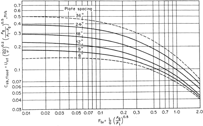
Figure 3.35 Capacity factor for flooding of sieve trays from Fair and Matthews (1958) (Reprinted by permission from Petroleum Refiner, copyright 1958, Gulf Pub. Co.)
To estimate the column diameter without a simulator, McCabe-Thiele approximate results are used. In this method, the flowrates are constant in each section of the column, so there are only two possible calculations, above and below the feed. An equation has been suggested to determine the limiting (larger diameter) section (Wankat, 2017). Intuitively, it may seem that the section with the larger molar flowrates will require a larger diameter. However, while the chemistry of phase equilibrium is based on molar flows and compositions, equipment sizing is based on mass flow-rates. Therefore, the molecular weight also affects the mass flowrate. Additionally, based on the relationship between mass flowrate and velocity, ![]() , the density affects the velocity, so a large temperature difference can be significant. Finally, especially in vacuum columns, the pressure drop can be a large fraction of the column pressure, which means that the vapor density can change significantly through the column. In general, the most desirable feed conditions are saturated liquid, saturated vapor, or a vapor-liquid mixture, because the feed should match column conditions (saturated). This suggests that the molar flowrates below the feed will be larger than those above the feed. Quite often, the higher boiler, which is at the bottom of the column, has the larger molecular weight. Thus far, it seems like designing for the bottom of the column is limiting. However, the pressure and temperature at the bottom of the column are both larger. For an ideal gas, the density ρ = PM/RT, where M is the molecular weight, so, depending on the exact numbers, the effects of temperature and pressure may offset. For vacuum columns, the pressure and therefore density will be significantly smaller above the feed. While it is usually most desirable to design a column with a uniform diameter, vacuum columns often have different diameters, larger above the feed and smaller below the feed, because the velocity above the feed is so much larger than the velocity below the feed. In a standard column, if the diameters above and below the feed are not compatible, that is, one section is so far below flooding to create weeping, the feed can be made into a vapor-liquid mixture to equalize the mass flowrates in both sections. In multicomponent distillation columns, flowrates change on every tray, and there are methods such as pump-arounds that can be used to avoid localized flooding (Wankat, 2017). At the level of the estimated diameter calculation, it is probably best to determine the diameter both above and below the feed.
, the density affects the velocity, so a large temperature difference can be significant. Finally, especially in vacuum columns, the pressure drop can be a large fraction of the column pressure, which means that the vapor density can change significantly through the column. In general, the most desirable feed conditions are saturated liquid, saturated vapor, or a vapor-liquid mixture, because the feed should match column conditions (saturated). This suggests that the molar flowrates below the feed will be larger than those above the feed. Quite often, the higher boiler, which is at the bottom of the column, has the larger molecular weight. Thus far, it seems like designing for the bottom of the column is limiting. However, the pressure and temperature at the bottom of the column are both larger. For an ideal gas, the density ρ = PM/RT, where M is the molecular weight, so, depending on the exact numbers, the effects of temperature and pressure may offset. For vacuum columns, the pressure and therefore density will be significantly smaller above the feed. While it is usually most desirable to design a column with a uniform diameter, vacuum columns often have different diameters, larger above the feed and smaller below the feed, because the velocity above the feed is so much larger than the velocity below the feed. In a standard column, if the diameters above and below the feed are not compatible, that is, one section is so far below flooding to create weeping, the feed can be made into a vapor-liquid mixture to equalize the mass flowrates in both sections. In multicomponent distillation columns, flowrates change on every tray, and there are methods such as pump-arounds that can be used to avoid localized flooding (Wankat, 2017). At the level of the estimated diameter calculation, it is probably best to determine the diameter both above and below the feed.
The curves in Figure 3.35 have been fit to the equation (Wankat, 2017):
where the constants are given in Table 3.7 for the different tray spacings.
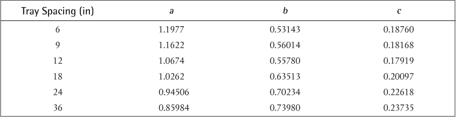
Table 3.7 Constants in Equation (3.58) (Wankat, 2017)
The parameter Flv is defined as

where L and V are molar flowrates, and ML and MV are molecular weights used to convert the molar flowrates to mass flowrates.
The nomenclature in Equation (3.59) and Figure 3.35 must be understood. First of all, throughout the history of separations, the variables V and G have been used somewhat interchangeably. V stands for vapor, while G stands for gas. V is being used in this chapter for all gas-vapor phases, but the original correlation of Fair and Matthews (1958) used G. On the x-axis of Figure 3.35, it is assumed that L and G are in mass units; Equation (3.59) expresses this clearly. On the y-axis of Figure 3.35, the parameter Csb,flood, which is abbreviated here as Csb,f, is

where uf is the flooding velocity in ft/sec, and σ is the surface tension of the liquid phase in dyne/cm2. The units of Equation (3.60) are exactly as stated; there is no metric equivalent available. Since the surface tension term is raised to a small power, only a small amount of error is introduced by assuming the entire term is unity.
The algorithm to determine the column diameter required is as follows:
1. Determine all internal flowrates in molar units. For distillation, this involves knowing the reflux ratio and the feed condition. For mass separating agents, the flowrates are likely given. Convert these to mass units. For distillation, it is usually assumed that the molecular weights in the vapor and liquid phases are equal, because the phases are not that different in composition. For mass separating agents, especially in dilute solutions, the molecular weight is approximately that of the solvent. (This may not be true for non-dilute vapor phases.)
2. Determine the liquid and vapor densities. The liquid density must be found from a reference. The vapor density can be estimated using the ideal gas law or another equation of state. The top and bottom temperatures and pressures are used, depending on which section the calculation is based.
3. Calculate Flv using Equation (3.59).
4. Use Equation (3.58) or Figure 3.35 to determine Csb,f.
5. Calculate uf (which will be in ft/sec) from Equation (3.60). If metric units are desired, convert it to m/s.
6. Calculate the actual velocity (uactual) as a percentage of the flooding velocity.
7. Calculate the column active area from
where VMV is the mass flowrate ![]() .
.
8. Determine the actual column area as actual area = active area/fraction active area.
9. Determine the column diameter from the actual area.
A distillation column that has a total condenser and a partial reboiler is fed 500 kmol/h of an equi-molar mixture of pentane and hexane. The feed is saturated liquid. It is necessary to produce outlet streams containing 95 mol% pentane and 99 mol% hexane. The distillation column contains a partial reboiler and a total condenser and operates at 1.4 times the minimum reflux ratio, which is a reflux ratio of 1.06. It has been determined that the column requires 15 equilibrium stages with the feed on Stage 5. The pressure at the bottom of the column is 2 bar. Assume that the McCabe-Thiele approximation is valid.
a. Determine the exit flowrates, D and B.
b. Determine all of the internal flowrates.
c. Determine the required column diameter for sieve trays with a 24-in tray spacing operating at 75% of flooding with 88% active area.
Data provided:

Solution
Figure E3.4 illustrates this column.
a. The outlet flowrates are obtained from an overall mole balance and a pentane mole balance.
The result is that D = 261 kmol/h and B = 239 kmol/h.
b. The internal flowrates are calculated from the top to the bottom, since the reflux ratio is the additional piece of information needed to start the calculation. Since R = L/D, and R and D are known, L = (1.06)(261) = 277 kmol/h. From a mass balance on the condenser, V = L + D, V = 538 kmol/h. Since the feed is saturated liquid, it is assumed that all of the feed goes to the bottom of the column. Therefore, ![]() kmol/h, and
kmol/h, and ![]() kmol/h. If the feed contained a vapor-liquid mixture, then the vapor flowrate above the feed would be larger than that below the feed by the flowrate of vapor in the feed. If the feed was saturated vapor, then the liquid flowrate would be assumed identical between the top and bottom, and the vapor flowrate above the feed would be the vapor flowrate below the feed plus the feed. These flowrates are all needed for the flooding calculation to determine the column diameter.
kmol/h. If the feed contained a vapor-liquid mixture, then the vapor flowrate above the feed would be larger than that below the feed by the flowrate of vapor in the feed. If the feed was saturated vapor, then the liquid flowrate would be assumed identical between the top and bottom, and the vapor flowrate above the feed would be the vapor flowrate below the feed plus the feed. These flowrates are all needed for the flooding calculation to determine the column diameter.

Figure E3.4 Illustration of Example 3.4
c. Since all of the liquid feed goes to the bottom of the column, the initial design will be for the bottom of the column, because it is assumed that the flowrates will be higher below the feed, requiring a larger diameter. For completeness, the top diameter will also be determined.
To use Equation (3.59), the vapor density must be calculated. Ideal gas will be assumed, so that
In Equation (E3.4c), the molecular weight of hexane is used for the bottom of the column, and the bottom temperature is obtained from Antoine’s equation at 2 atm for pure hexane. This is clearly an assumption. On the bottom tray, since there is almost pure hexane, the assumption may be valid. However, the temperature decreases on every tray above the feed, as does the pressure and the molecular weight (since pentane has a lower molecular weight). So, without knowing the pressure drop, the pressure is assumed to be uniform throughout the column. The small change in vapor density within the column is not significant relative to the other assumptions in this approximate calculation. Additionally, the bottom temperature is really the bubble point of the mixture. Overall, this method is clearly an estimation. In a process simulator, for example, the calculation that follows is performed rigorously on every tray.
From Equation (3.59),

The molecular weight is omitted from the calculation in Equation (E3.4d), because it is assumed that the compositions of vapor and liquid on a tray are about the same, so the average molecular weights are about the same. This only holds for distillation. For absorbers and strippers, the molecular weight must be included, and a good starting approximation is the molecular weight of the solvent.
Applying Equation (3.58) for 24-in tray spacing, using the values in Table 3.7, yields Csb,f = 0.3054. The flooding velocity is then calculated from Equation (3.60):

The term involving surface tension is assumed to be unity. In the worst case, if water was involved, with a surface tension of 72 dyne/cm2 at room temperature, the term would be (72/20)0.2 = 1.3. For organic molecules, the surface tension at room temperature is on the order of 30 dyne/cm2, so omitting this term is within the approximations of this calculation. At 75% of flooding, the actual vapor velocity is u = 0.75(3.025 ft/sec)(0.3048 m/ft) = 0.692 m/s. Now, the active area is calculated from

So, the actual area, Aactual, is 3.28/0.88 = 3.73 m2. Solving for the diameter,
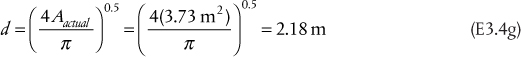
If the entire calculation was repeated for the top, using the molecular weight of pentane (72 kg/kmol) and the top section density (5.23 kg/m3, calculated using the top temperature of 58.05°C) and flowrates, the top diameter would be 1.73 m. To determine whether the top section will perform correctly, the actual velocity above the feed is calculated assuming that the bottom active area is the same as the top active area, that is, the column is at uniform diameter,
and the percentage of flooding in the top section is (0.63 m/s)/[(0.3048 m/ft)(3.025 ft/sec)] = 0.68. Since this is not small enough for weeping to occur, then a 2.18 m diameter column will work.
3.3.2.3 Tray Efficiency
Real trays are not 100% efficient, which means that they are not equilibrium trays. In a column, the tray efficiencies must be known to determine the number of actual trays. Individual tray efficiencies can be defined on the basis of the fractional approach to equilibrium, and these are called Murphree efficiencies:
where the numerators represent the actual mole fraction change on a tray, and the denominators represent the mole fraction change on a tray if equilibrium is reached on the tray. The subscripts V and L represent a vapor-phase and a liquid-phase basis, respectively. While these definitions make intuitive sense, they are not very useful for a variety of reasons. One reason is that they differ for every tray, and experimental results would be needed for every tray before the design of a column.
Another method for estimation is to use empirical results gathered over many years of practice, and these results were presented by O’Connell (1946). The results are presented in Figure 3.36, which are for overall, average column efficiencies. There are different correlations for distillation columns and for absorbers/strippers. The parameter for distillation is αμ, where α is the relative volatility of the key components (only two components in binary distillation), and μ is the viscosity of the feed in cP (centipoise). The efficiency decreases as the relative volatility increases because more mass must be transferred to reach equilibrium, and the efficiency decreases as the viscosity increased because mixing is more difficult, which lowers the mass transfer rate. A curve fit of the points shown (in percent) has been suggested (Couper et al., 2012, page 471):
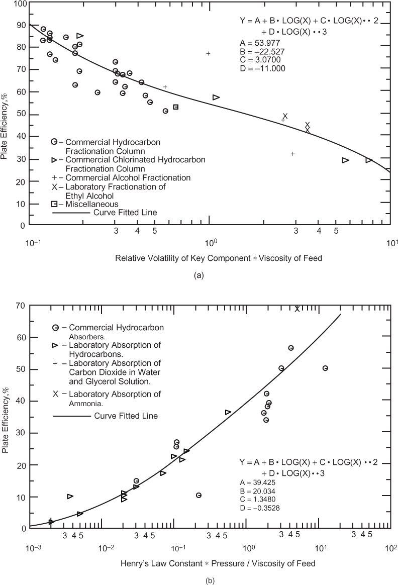
Figure 3.36 Efficiencies of distillation columns and absorber-strippers (Reproduced with permission from Couper et al. [2012])
An alternative curve fit has also been suggested (Wankat, 2017):
For absorbers, the parameter is HP/μ, where H is Henry’s law constant (in lbmol/ft3/atm), P is the pressure (in atm), and μ is the viscosity (in cP).
Estimate the efficiency of the distillation column in Example 3.4. The feed viscosity is 0.25 cP. Then, calculate the number of actual trays in the column and the column height.
Solution
The relative volatilities must be calculated first. The relative volatility is α = K5/K6. Assuming constant pressure in the column, ![]() . Using the top temperature of 58.05°C, αtop = 2.83, and using the bottom temperature of 92.62°C, αbottom = 2.46. The geometric average of the top and bottom relative volatilities is usually used, which yields α = 2.64; however, since the two numbers are so close, the algebraic average is virtually the same number. Using Equation (3.64) yields 58.2%, and using Equation (3.65) yields 57.9%. So, the actual number of trays is based on 14 equilibrium trays, since one of the equilibrium stages is the partial reboiler. The result is about 24 trays. For a 24-in tray spacing (0.6096 m), the column height is 14.6 m, which is a height-to-diameter ratio of 14.6/1.94 = 7.23, which is well within the limit of typical operation.
. Using the top temperature of 58.05°C, αtop = 2.83, and using the bottom temperature of 92.62°C, αbottom = 2.46. The geometric average of the top and bottom relative volatilities is usually used, which yields α = 2.64; however, since the two numbers are so close, the algebraic average is virtually the same number. Using Equation (3.64) yields 58.2%, and using Equation (3.65) yields 57.9%. So, the actual number of trays is based on 14 equilibrium trays, since one of the equilibrium stages is the partial reboiler. The result is about 24 trays. For a 24-in tray spacing (0.6096 m), the column height is 14.6 m, which is a height-to-diameter ratio of 14.6/1.94 = 7.23, which is well within the limit of typical operation.
3.3.2.4 Pressure Drop
As stated previously, liquid flows down through a column due to gravity, and vapor flows upward due to a pressure difference. While the top and bottom pressures are determined by the bubble points of the top and bottom trays, they are not independent of the hydraulics on the trays. Each tray has a pressure drop that the vapor must overcome, and the total pressure drop is the sum of the pressure drops on the trays. Therefore, it is necessary to understand something about the tray hydraulics to understand the pressure drop on each tray.
Figure 3.37 is a schematic of the liquid flow across a tray. The vapor flowing upward must overcome the downcomer head (hdc), which is the sum of all of the other heads shown in Figure 3.37,

where
hweir = weir height, the dominant term
hcrest = crest over weir, the level of liquid above the top of the weir
hgrad = hydraulic gradient, difference in level from the downcomer side and the weir side
hdu = frictional loss of liquid flowing out of downcomer
hdry = the “dry” head, the head to get vapor through holes in tray
If the weir height is assumed to be the dominant contribution to the pressure drop, and assuming that all weir heights are the same, the column pressure drop becomes
where the subscripts above and below refer to the location in the tower relative to the feed. The liquid densities are used as a conservative estimate, since the portion of the tray containing a froth (two-phase, vapor-liquid mixture) is unknown in an initial design. Since the estimation methods presented here are based on the properties of the more volatile component above the feed tray and the less volatile component below the feed tray, their liquid densities would be used for the appropriate section of the column.
Estimate the pressure drop in the column of Examples 3.4 and 3.5 if the weir height is 4 in.
Solution
Equation (3.67) defines the pressure drop. Since there are 14 equilibrium trays with the feed on Tray 5, when applying the efficiency to convert to 24 actual trays, the feed is located proportionally at the same location. So the feed is on Tray 5(24/14) = 8.57 ≈ 9. Given that Equation (3.67) is an estimate, there would be little difference in rounding down to the feed on Tray 8. Using the densities in Example 3.4, Equation (3.67) becomes
In Example 3.4, the pressure was assumed constant at 2 atm throughout the column. Applying this pressure drop would change the calculated diameter slightly.
3.3.2.5 Condensers and Reboilers
The impact of the reboiler and condenser on the design and operation of a distillation column is often overlooked in basic textbooks. They are just heat exchangers, the design of which was discussed in Chapter 2. Figure 3.38 shows the T-Q diagrams for a typical condenser and reboiler. It is assumed that the streams being reboiled and condensed are pure components, hence the horizontal lines representing constant temperature. If those streams were not pure, the lines would be slightly inclined, representing the difference between the bubble-point and dew-point temperatures. It is also assumed that the condensate is not subcooled, which might happen in some applications.
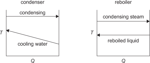
For the reboiler, the energy balances and design equations are
where the subscript R denotes the reboiler, the subscript p denotes the process stream, and the subscript s denotes steam, which is a standard source of heat. The overbars indicate the bottom of the column. Built in to Equation (3.68) is the assumption that all phase changes are between saturated liquid and saturated vapor. The log-mean subscript is omitted from the temperature difference, because the temperature difference between the two streams is constant at all points, and thus ΔTlm = ΔT.
Once the flowrate of the process stream is known, since the latent heat can be found in the literature, the heat duty, Q, is known. If the heat transfer coefficient and the available steam temperature are known, then there is a unique correspondence between Tp and A. So, a reboiler can be designed for any desired value of Tp. There is an exact pressure for this value of Tp, based on Antoine’s equation. Care must be taken to keep (Ts − Tp) from being too large to avoid film boiling, as discussed in Chapter 2.
The pressure in the condenser is obtained from the pressure in the reboiler minus the column pressure drop. The column pressure drop is not arbitrary but is related to the weir height, as discussed the previous section. From Antoine’s equation, the condensing temperature is then known. In the condenser, the energy balances and design equation are
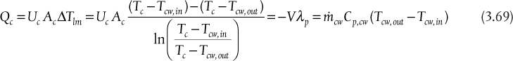
where the subscript c denotes the condenser or condensation temperature, and the subscript cw denotes cooling water, which is the most desirable heat sink in a condenser. Therefore, if the heat transfer coefficient is known, there is only one condenser area that will satisfy Equation (3.69) for the calculated Tc.
When simulating a column, the pressure drop is an input variable. However, it is not known until the trays are designed, but the pressure drop is dependent on the number of trays, which is not known until the column is simulated. Therefore, column design is an iterative process, and this is not the only source of iterations. As a first approximation, a pressure drop could be assumed and the weir height calculated after determining the number of trays and feed location. If the weir height is reasonable, the result may be sufficient for a first step. If not, then the pressure drop must be changed to correspond to a reasonable weir height.
The condenser and reboiler also affect the pressure in the column. In a chemical plant, the least expensive source of cooling in the condenser is usually process cooling water. Air can be used, but the heat transfer coefficient from a gas is much smaller than from a liquid. While the following values may differ from plant to plant and seasonally, typically, process cooling water is available at 30°C and is returned at 40°C. (The returned cooling water can be cooled back to 30°C by evaporating about 2%, so, other than makeup for the 2% evaporated, it is a closed loop.) If a 10°C approach temperature between the cooling water and the condensation temperature is desired (Figure 3.38), then the top column pressure must be high enough for the boiling point of the top component to be 50°C (bubble point of mixture at top). Quite often, distillation of low-boiling components, such as ethane-ethylene or propane-propylene, are run at significant pressures to make the top temperature around 50°C.
Columns can also be run at vacuum by using either a steam ejector (covered in Chapter 5) or a vacuum pump at the top of the column. There are two possible reasons for running a column under vacuum. One is that a component in the distillation is temperature sensitive. For example, acrylic acid spontaneously polymerizes at 90°C. To keep the temperature below 90°C, the pressure must be 0.16 bar. So, in the purification of acrylic acid from acetic acid, the undesired product of a side reaction, the column is run at vacuum. (In this particular example, acrylic acid is the higher boiler, so it is the bottom pressure that is at 0.16 bar!) A second reason is the available steam temperature for high boilers. Typically, the highest pressure, saturated steam available for a reboiler is around 250°C. For example, phthalic anhydride’s normal boiling point is 295°C. Therefore, the column that purifies phthalic anhydride is run at around 0.4 bar, where phthalic anhydride boils at around 240°C.
Calculate the heat duty for the condenser and the reboiler and their required heat transfer areas. In the condenser, cooling water is used, entering at 30°C and leaving at 40°C. In the reboiler, low-pressure steam is used, which is condensed at 160°C.
Data provided:
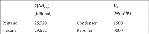
Solution
Since the compositions are known at the top and at the bottom of the column from Example 3.4, if ideal mixture is assumed, which is most likely valid at the relatively low pressure of the column with non-polar hydrocarbon components, the heats of vaporization can be weighted by the mole fractions (Figure E3.4).


It is observed that the absolute values of the heat duties are very close numerically. This is expected. They should be on the same order of magnitude. If they are not, it suggests that the feed is very different from the column conditions, probably either very subcooled or very superheated.
Figure E3.7 shows the T-Q diagrams for the condenser and the reboiler. For the condenser,
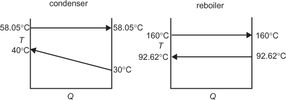

so Ao (condenser) = 113.8 m2,
and for the reboiler,
so Ao (reboiler) = 21.9 m2.
The utility flowrates are obtained from the respective energy balances. For the condenser,

so ![]() 92.5 kg/s, and for the reboiler,
92.5 kg/s, and for the reboiler,
so ![]() = 2.12 kg/s.
= 2.12 kg/s.
3.3.3 Packed Towers
Another method for contacting vapors and liquids to accomplish separations is a packed tower. A packed tower is a large, cylindrical vessel packed with inert material. While in tray towers, mass transfer area is created by the gas bubbles within the liquid on the tray, the concept in a packed tower is that liquid coats the solid, packing surface creating mass transfer area for the vapor passing countercurrently. Just as in a tray tower, liquid flows down by gravity and the vapor flows upward due to a pressure gradient.
There are several other differences between packed towers and tray towers. Packed towers flood, but entrainment and weeping do not occur. In general, packed towers have lower pressure drops than tray towers. One problem with packed towers is the potential for flow maldistribution, which is the uneven distribution of liquid across the cross section, which can create regions of uncoated, dry solid, reducing the expected mass transfer area. Since flow maldistribution manifests more often in larger-diameter towers, historically, tray towers were used for larger-diameter (i.e., larger-capacity) columns, such as distillation in oil refineries, and packed towers were used for smaller-diameter (i.e., smaller-capacity) columns, such as removing pollutants from exhaust streams. Flow maldistribution is also related to the column diameter and the packing material diameter. If column diameter/packing diameter >40, maldistribution is more likely. One method that can be used to mitigate flow maldistribution in larger diameter columns is to have the packing in sections with the liquid collected and redistributed across the cross section throughout the column. This is illustrated in Figure 3.39.

Figure 3.39 Internals of a packed column with structured packing showing redistributor (Stichlmair and Fair [1998])
3.3.3.1 Packing Types and Shapes
There are two types of packing types, random packing and structured packing. Random packings are randomly dumped into the cylindrical vessel. As illustrated in Figure 3.40, there are more shapes for random packings than can be imagined. The idea is to get the maximum mass transfer area, the largest mass transfer coefficient, and the lowest pressure drop. The random packing material can be plastic, metal, or ceramic, and the choice is based on cost and chemical compatibility.
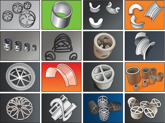
Figure 3.40 Some shapes of random packings (Reprinted by permission from Jiangxi Jintai Special Material LLC, copyright 2005, all rights reserved)
A more recent development is structured packings, which come in sections that slide into the cylindrical vessel. One key advantage of structured packings is a very-low pressure drop. Figure 3.41 illustrates a structured packing.
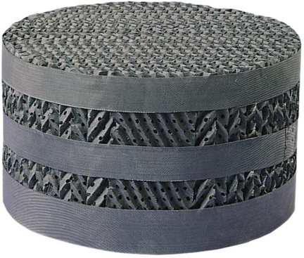
Figure 3.41 Example of a structured packing (https://www.sulzer.com/en/Products-and-Services/Separation-Technology/Structured-Packings/Gauze-Packings-BX-CY-BXPlus-AYPlus-DC-Hyperfil-and-Multifil)
3.3.3.2 Height and Diameter
Table 3.2 shows four methods for obtaining the height of a packed column. The number of transfer units depends on the equilibrium, as discussed in Section 3.2.2.1. The height of a transfer unit depends on the mass transfer, and one method for calculating the height of a transfer unit is also presented in Section 3.2.2.1. The height of the packed portion of the column is the product of the height of a transfer unit and number of transfer units, as shown in Table 3.2. For a distillation column, the heights above and below the feed are calculated separately and added. For an absorber or stripper, since there is only one section, just one height is calculated.
There is another method that can be used for calculating the height of a packed tower, the height equivalent to a theoretical plate (HETP). In this method, the number of trays (also called plates) is calculated as if designing a tray tower. If the HETP can be calculated, the tower height is
The expression for HETP is
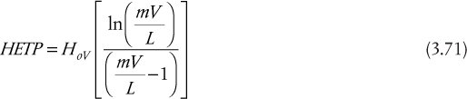
where HoV is defined in Table 3.2, and the flowrates L and V are molar flowrates. The mass transfer coefficient must still be known, since it is in HoV, but the HETP expression replaces the tedious NoV calculation described in Section 3.2.2.1. A possible heuristic is that HETP ≈ 0.5 m. Another heuristic might be HETP (ft) ≈ 1.5 (packing size, inches).
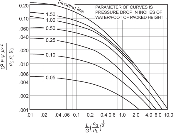
Figure 3.42 Generalized flooding and pressure drop correlation for packed columns (Reprinted with permission from Eckert [1970]. Reproduced with permission by the American Institute of Chemical Engineers)
The diameter of a packed tower is based on a flooding calculation. The concept is identical to that for tray towers, but the empirical correlation is different. A graphical representation of the flooding limit is shown in Figure 3.42. The important line is the flooding line and a curve fit has been presented (Wankat, 2017) that corresponds to the equation
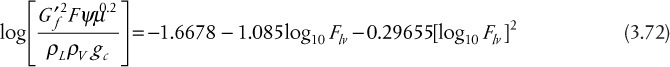
where Flv is defined in Equation (3.59), Gf′ is the superficial mass flowrate of vapor at flooding (could be called Vf′) in lb/ft2/sec (area unit is cross-sectional area of tower), the densities are in lb/ft3, the viscosity (μ) is in cP, ψ is the inverse of the specific gravity of the liquid (ρwater/ρL), F is a packing factor found in Table 3.8, and gc is the unit conversion 32.2 ft lbm/(lbfsec2). The units must be exactly as stated in this empirical correlation, and they are not consistent with each other. The algorithm is as follows:
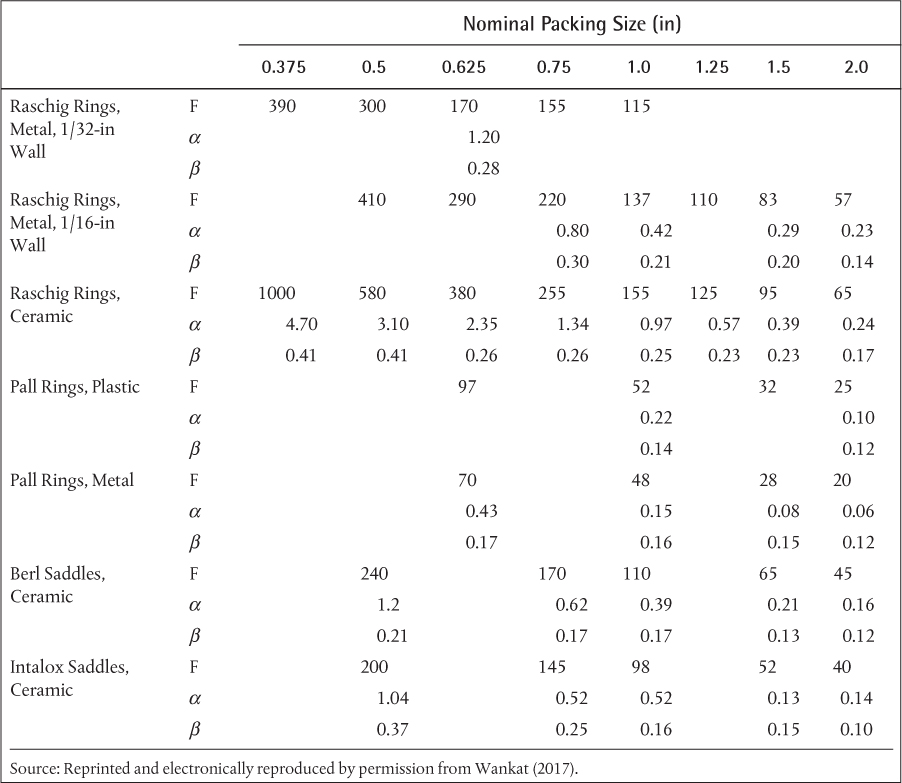
1. Determine all internal flowrates in molar units. For distillation, this involves knowing the reflux ratio and the feed condition. For mass separating agents, the flowrates are likely given. Convert these to mass units. For distillation, it is usually assumed that the molecular weights in the vapor and liquid phases are equal, because the phases are not that different in composition. For mass separating agents, especially in dilute solutions, the molecular weight is approximately that of the carrier solvent (non-absorbing component).
2. Determine the liquid and vapor densities. The liquid density must be found from a reference. The vapor density can be estimated using the ideal gas law or another equation of state. The top and bottom temperatures and pressures are used, depending on which section the calculation is based.
3. Calculate Flv from Equation (3.59).
4. Use Equation (3.72) or Figure 3.42 to determine the parameter in the brackets.
5. Solve for Gf′, which has units lb/ft2/sec. This is the value of G′ at flooding.
6. Calculate the actual value of G′ as a desired percentage of the flooding velocity (typically 70%–80% of flooding for a packed tower).
7. Calculate the area from
where G is the mass flowrate of vapor in the column.
8. Determine the column diameter from the area.
Just as for tray towers, for a distillation column, this calculation should be done both above the feed and below the feed and a diameter chosen that satisfies both results. Since there is no lower percentage of flooding limit (no weeping), choosing an appropriate diameter is easier for a packed tower than for a tray tower.
3.3.3.3 Pressure Drop
The pressure drop can be estimated from Figure 3.42. The units are inches H2O/ft packed height. The curves below the flooding line provide the values for the pressure drop. Once the flooding G′ is obtained, the actual value of G′ is obtained from the desired flooding percentage. Then, a new y-axis is obtained, and the value of Flv is already known, so the pressure drop is obtained. Then the overall pressure drop is obtained by multiplying that value by the column height.
An empirical correlation for the pressure drop has been presented (Wankat, 2017).
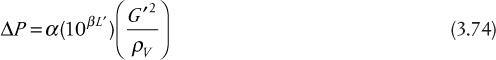
where α and β are listed in Table 3.8. L′ and G′ are superficial mass flowrates in lb/ft2/sec, the density is lb/ft3, and the resulting pressure drop is in inches H2O/ft packed height.
An air stream flowing at 1500 kmol/h containing benzene vapor is to be scrubbed in a packed bed using 1-in, ceramic Berl saddles using 250 kmol/h of hexadecane as the solvent. The mole fraction of benzene in the inlet air is 0.01, and the required outlet mole fraction is 0.0005. The hexadecane is being returned to the scrubber from a stripper, so the inlet mole faction of benzene in hexadecane is 0.0001. The column may be assumed to operate at 150 kPa and 35°C. Raoult’s law may be assumed to define the benzene equilibrium.
a. Determine the diameter of the packed column for 75% of flooding.
b. Determine the pressure drop per unit height in the column.
Data provided:

a. The method discussed in Sections 3.3.3.2 and 3.3.3.3 is used. Just as in a tray tower, the term Flv must be calculated first. So, the density of the gas phase must be estimated. Since the system is dilute, the density of air can be used. An average molecular weight should be used; however, given the approximate nature of this calculation, using the molecular weight of air is reasonable. So,
From Equation (3.59),

From Equation (3.72),

so that
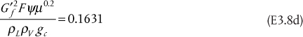
and solving for the flooding superficial mass flowrate,
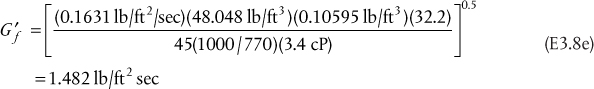
where the densities have been converted into the required units, and the value of F, the packing factor, 45, is found in Table 3.8. For 75% of flooding, then G′ = 1.111 lb/ft2/sec. The area is found by using Equation (3.73):
so, the diameter is found to be 5.52 ft.
b. The pressure drop is found from Equation (3.74), using the parameters α and β from Table 3.8.
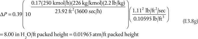
This is not a small pressure drop, since the pressure drop in a 50 ft column would be just under 1 atm. It might be better to use a larger packing size to reduce the pressure drop. However, this would reduce the packing factor, thereby increasing the flooding velocity, which increases the column diameter. Ultimately, the decision would be based on economics.
3.3.4 Tray Tower or Packed Tower?
The choice between tray towers and packed towers depends on several variables, and some of the guidelines may be conflicting. Traditionally, packed towers were used for smaller-diameter columns because of the flow maldistribution discussed earlier. Therefore, they were used for lower-capacity operations. However, structured packing combined with liquid flow distributors have made it possible to use packed towers for larger-capacity operations. The lower pressure drop in packed towers makes them uniquely applicable to vacuum operations. Packed towers do flood; however, they do not weep, so it may seem that they are more flexible for operations that might have to be scaled down. However, there is a minimum liquid load (flowrate) for packed towers, and, if distributors are used to avoid flow maldistribution, there is a window of flowrate operation, just as for tray towers, but for different reasons (Stichlmair and Fair, 1998). This is one reason why tray towers are preferred for larger capacity operations.
Tray towers were traditionally used for larger-capacity (larger-diameter) operations. Trays are easier to clean than packing, so trays are more applicable to fouling operations. In a tray tower, access points are built in for maintenance (manways) and cleaning during shutdown. However, in a packed tower, the packing must be removed for the same access. In more advanced distillation operations, such as reactive distillation, adding heat transfer capability to remove heat produced by an exothermic reaction is easier in a tray tower by inserting a liquid take-off at a given tray and pumping the liquid through an external heat exchanger and returning the liquid to another tray.
Ultimately, the choice between a tray tower and a packed tower comes down to the economics. However, constraints for a specific application must also be considered.
3.3.5 Performance of Packed and Tray Towers
In the day-to-day operations of a chemical plant, process conditions change. For example, the rate of production may have to increase or decrease. Reasons for an increase in production include an increased demand for the product or a need to meet contracted customer demand when a similar plant within the company goes off line. These performance problems were discussed in the context of fluid flow equipment and heat exchangers in Chapters 1 and 2, respectively.
If a distillation column must be scaled-up (scaled-down) at constant product purities, the material balance requires that inlet and outlet flowrates increase (decrease) by the same amount. The question is how the output changes based on equipment performance. Clearly, there is a limit to scale-up of a distillation column based on the flooding limit. If the inlet flowrate to a distillation column increases at constant composition, and if the outlet compositions are maintained, the reflux rate increases, since the reflux ratio (L/D) stays constant. Therefore, all internal flows increase, making flooding a real possibility. If, for example, a column was designed for 75% of flooding, a 10% to 15% scale-up might be possible, assuming that it is desired to keep the flooding percentage less than 85% to 90% to avoid loading. For scale-down, there might be more flexibility, since weeping does not typically occur until <40% of flooding, with the exact value dependent on the tray type.
However, the situation is not that simple. In Section 2.8, the performance of heat exchangers was discussed, and it was seen that changing the inlet flowrate to a heat exchanger affects the temperatures of both streams and the total heat load. Since it has been shown that the condenser and reboiler affect the pressure of the column, then scale-up or scale-down of a distillation column involves much more than flooding. Therefore, the performance of a distillation column cannot be analyzed without consideration of the performance of both the condenser and reboiler. This is illustrated with a case study.
Case Study
The distillation column illustrated in Figure 3.43 is used to separate benzene and toluene. It contains 35 sieve trays, with the feed on Tray 18. The relevant flows are given in Table 3.9. Your assignment is to recommend changes in the tower operation to handle a 50% reduction in feed. Overhead composition must be maintained or exceed the current specification of 0.996 mole fraction benzene. Cooling water is used in the condenser, entering at 30°C and exiting at 45°C. Medium-pressure steam (185°C, 1135 kPa) is used in the reboiler. The operating conditions of the tower before reduction in feed are in Table 3.9.

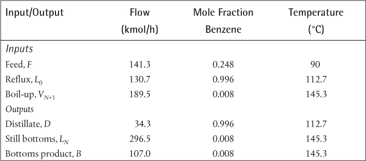
Table 3.9 Operating Conditions for Process in Figure 3.43
Among the several possible operating strategies for accomplishing the necessary scale-down are the following:
1. Scale down all flows by 50%. This is possible only if the original operation is not near the lower velocity limit that initiates weeping or reduced tray efficiency. If 50% reduction is possible without weeping, reduced tray efficiency, or poor heat-exchanger performance, this is an attractive option.
2. Operate at the same boil-up rate. This is necessary if weeping or reduced tray efficiency is a problem. The reflux ratio must be increased in order to maintain the reflux necessary to maintain the same liquid and vapor flows in the column. In this case, weeping, lower tray efficiency, or poor heat-exchanger performance caused by reduced internal flows is not a problem. The downside of this alternative is that a purer product will be produced and unnecessary utilities will be used. Increasing the reflux ratio during scale-down increases the utility cost or the column per unit product.
In Example 3.9, the analysis will be done by assuming that it is possible to scale down all flows by 50% without weeping or reduced tray efficiency.
Estimate the pressure drop through the column. To what weir height does this correspond?
Solution
Interpolation of tabulated data (Perry and Green, 1997) yields the following relationships for the vapor pressures in the temperature range of interest:
It is assumed that the bottom is pure toluene and the distillate is pure benzene. This is a good assumption for estimating top and bottom pressures given the mole fractions specified for the distillate and bottoms. Therefore, at the bottom temperature of 141.7°C, the vapor pressure of toluene, and hence the pressure at the bottom of the column, is 227.2 kPa. At the top temperature of 104.2°C, the vapor pressure of benzene, and hence the pressure at the top of the column, is 204.8 kPa.
Because there are 35 trays, the pressure drop per tray is
If it assumed that the weir height is the major contribution to the pressure drop on a tray, then
where h is the weir height. Assuming an average density of 800 kg/m3, then
This is a typical weir height and is consistent with the assumption that the weir height is dominant.
The pressure drop is assumed to remain constant after the scale-down because the weir height is not changed. In practice, there is an additional contribution to the pressure drop due to gas flow through the tray orifices. This would change if column flows changed, but the pressure drop through the orifices is small and should be a minor effect. Examples 3.10 and 3.11 illustrate how the performance of the reboiler and condenser affect the performance of the distillation column.
Analyze the reboiler to determine how its performance is altered at 50% scale-down.
Solution
Figure E3.10 shows the T-Q diagram for this situation. Because the amounts of heat transferred for the base and new cases are different, the Q values must be normalized by the total heat transferred in order for these profiles to be plotted on the same scale. The solid lines are the original case (subscript 1). For the new, scaled-down case (subscript 2), a ratio of the energy balance on the reboiled stream for the two cases yields
If it is assumed that the latent heat is unchanged for small temperature changes, then Q2/Q1 = 0.5, because at 50% scale-down, the ratio of the mass flowrates in the reboiler is 0.5. The ratio of the heat transfer equations yields
In Equation (E3.10b), it is assumed that the overall heat transfer coefficient is constant. It is assumed here that U ≠ f(T). This assumption should be checked, because for boiling heat transfer coefficients with large temperature differences, the boiling heat transfer coefficient may be a strong function of temperature difference.
From Equation (E3.10b), it is seen that ΔT2 = 21.7°C. Therefore, for the reboiler to operate at 50% scale-down, with the steam side maintained constant, one possible option is that the boil-up temperature must be 163.4°C. This is shown as the dotted line in Figure E3.10.
From the vapor pressure expression for toluene, the pressure at the bottom of the column is now 372.5 kPa. It would have to be determined whether the existing column could withstand this greatly increased pressure.
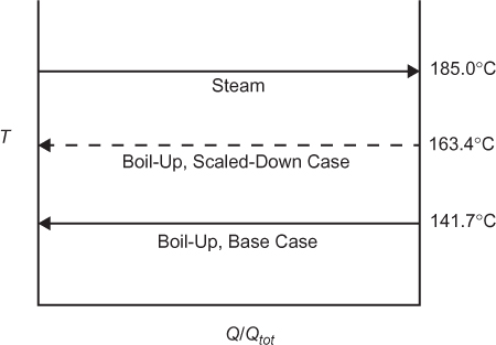
Figure E3.10 Temperature profiles in reboiler for Example 3.10
Example 3.10 shows that the reboiler operation requires that the pressure of the boil-up stream be increased. This is not the only possible alternative. All that is necessary is that the temperature difference be 21.7°C. This could be accomplished by reducing the temperature of the steam to 163.4°C. In most chemical plants, steam is available at discrete pressures, and the steam used here is typical of medium-pressure steam. Low-pressure steam might be at too low a temperature to work in the scaled-down column. However, the pressure and temperature of medium-pressure steam could be reduced if there were a throttling valve in the steam feed line to reduce the steam pressure. The resulting steam would be superheated, so desuperheating would also be necessary. This is usually accomplished by spraying water into the superheated steam. This system is called a desuperheater, and the benefit of a desuperheater is to permit flexibility in saturated steam conditions to facilitate process changes and process control. A change in a utility stream is almost always preferred to a change in a process stream, because it does not disrupt process operation at the design conditions.
The condenser is now analyzed in Example 3.11.
Using the results of Example 3.10, analyze the condenser for the scaled-down case.
Solution
Under the assumption that the pressure drop for the column remains at 22.4 kPa, the pressure in the condenser is now 350.0 kPa. From the vapor pressure expression for benzene, the new temperature in the condenser is 126.0°C. The remainder of the analysis is similar to Example 2.20. The T-Q diagram is illustrated in Figure E3.11. Because an organic is condensing, it is assumed that the resistance on the cooling water side is approximately equal to the resistance on the condensing side. The method presented can be used for any known heat transfer coefficients or any known ratio of heat transfer coefficients. Therefore,
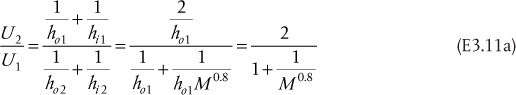
where ![]()
The ratio of the base cases for the energy balance on the condensing stream is

Figure E3.11 Temperature profiles in condenser for Example 3.11
Because the ratio of the mass flowrates is 0.5, and assuming that the latent heat is unchanged with temperature in the range of interest, Q2/Q1 = 0.5.
The ratio of the base cases for the energy balance and the heat-exchanger performance equation (Q = UAΔTlm) are, respectively,
Solution of Equations (E3.11c) and (3.11d) yields
M = 0.203
T = 66.9°C
Therefore, the cooling water rate must be reduced to 20% of the original rate, much lower than the actual scale-down. The outlet water temperature is increased by about 22°C. This would cause an unacceptable increase in fouling on the cooling water side, since 45°C is typically the maximum allowable return temperature due to fouling. Therefore, in this case, it may be better to use a higher reflux ratio rather than reduce the flows within the column.
Observation indicates that in order to operate the distillation column at 50% scale-down with process flows reduced by 50%, a higher pressure is required and the cooling water will be returned at a significantly higher temperature than before scale-down. The operating pressure of the column is determined by the performance of the reboiler and condenser.
Examples 3.10 and 3.11 reveal a process bottleneck at the reboiler that must be resolved in order to accomplish the scale-down. In the process of changing operating conditions (capacity) in a plant, a point will be reached where the changes cannot be increased or reduced any further. This is called a bottleneck. A bottleneck usually results when a piece of equipment (usually a single piece of equipment) cannot handle additional change. In this problem, one bottleneck is the high cooling water return temperature, which would almost certainly cause excessive fouling in a short period of time. Another potential bottleneck is tray weeping due to the greatly reduced vapor velocity. In addition to the solution presented here, there are a variety of other possible adjustments, or debottlenecking strategies, which follow with a short explanation for each.
1. Replace the Heat Exchangers: Equation (E3.10b) shows that a new heat exchanger with half of the original area allows operation at the original temperature and pressure. The heat transfer area of the existing exchanger could be reduced by plugging some of the tubes, but this modification would require a process shutdown. This involves both equipment downtime and capital expense for a new exchanger. Your intuitive sense should question the need to get a new heat exchanger to process less material. You can be assured that your supervisor would question such a recommendation.
2. Keep the Boil-Up Rate Constant: This would maintain the same vapor velocity in the tower. If the operation occurs near the lower velocity limit that initiates weeping or lower tray efficiency, this is an attractive option. The constant boil-up increases the tower separation. This option results in much smaller temperature and pressure changes but is somewhat wasteful, as approximately the same amount of reboiler and condenser energy is being used to process only 50% of the original material.
3. Introduce Feed on a Different Plate: This strategy must be combined with Option 4. The plate should be selected to decrease the separation and increase the bottoms concentration of the lower boiling fraction. This lowers the process temperature and increases the ΔT for heat transfer and the reboiler duty. This may or may not be simple to accomplish depending on whether the tower is piped to have alternate feed plates. As in Option 2, the reflux and coolant inputs will change.
4. Recycle Bottoms Stream and Mix with Feed: This strategy must be combined with Option 3. By lowering the concentration of the feed, the concentration of the low boiler in the bottoms can be increased, the temperature lowered, and the reboiler duty increased. This represents a modification of process configuration and introduces a new (recycle) input stream into the process.
The next series of examples involves the performance of an absorber. The same methodology would be used for a stripper.
An absorber is designed to be 20 m tall, and it is known that HoV is 4 m. The absorber is designed to treat 40 kmol/h of air containing acetone with a mole fraction of 0.002 and reduce the mole fraction to 0.0001. Pure water is the solvent, at a rate of 20 kmol/h. The column temperature is 26.7°C, and the pressure is 1.2 atm. Raoult’s law may be assumed to apply, and
It is now observed that the outlet mole fraction of acetone in the air is 0.0002. List as many possible causes of this situation as you can, assuming that only one fault exists at a time. Quantify what is happening in the column for each case, that is, what parameter is off and what is the off-specification value?
Solution
There are six possible single-parameter upsets (off-design conditions) that do not involve malfunctions within the packed bed equipment. All can be understood from the dilute, packed-bed absorber equation in Table 3.6:

which is valid for these dilute solutions. Since the bed height z = HoVNoV, NoV = 5. For the base case, at 26.7 + 273.15 = 299.85 K, P* = 0.339 atm. Therefore, m = P*/P = 0.283, and A = L/(mV) = 20/0.283/40 = 1.77. Since the water is pure, xin = 0 for the base case.
There are only three parameters in Equation (E3.12b), so the problem must be with one of these parameters. It is assumed that NoV is correct, since the most likely way that it could be incorrect is if HoV is incorrect, which would probably be due to an impediment to mass transfer, such as channeling or fouling. However, it was stated that equipment malfunctions were to be ignored.
One possibility is that every parameter on the right-hand side of Equation (E3.12b) is at design conditions but that yout = 0.004. This means that the absorber is removing the same fraction of acetone from the air, but that the mole fraction of acetone in the inlet air has doubled.
A second possibility is that every parameter on the right-hand side of Equation (E3.12b) is at design conditions, that yin is at design conditions, but that xin ≠0. Solution of Equation (E3.12b) yields xin = 0.00352. How could this happen? It is possible that the water is regenerated in a stripper and that the stripper is exhibiting a malfunction. If there was a stripper, the inlet water would certainly have small amounts of acetone, so a more likely scenario is that the inlet water has more acetone than expected. However, the concept is identical.
The third possibility is that A is not at design conditions. At yin = 0.002, yout = 0.0002, and NoV = 5, Equation (E3.12b) can be solved for A = 1.275. Since A = L/(mV), if A has decreased, then either L has decreased, V has increased, or m has increased. Holding two of these parameters at the original values while solving for the third parameter yields either L = 14.43 kmol/h, V = 55.45 kmol/h, or m = 0.392. The first two values make intuitive sense, since a decrease in solvent rate or an increase in gas to be treated will both make the absorber remove less solute, assuming all other parameters remain unchanged. However, the increase in vapor flowrate is 38%. If this really occurred, flooding could be occurring. Since flooding would probably cause the column to malfunction to the extent that there would be no liquid flow downward, it is likely that such a large increase in V is not the cause of the problem.
The value of m can change only if the temperature or pressure changes. Since the new value of m = P*/P = 0.392, the new pressure can be found as P = 0.865 atm at the original temperature, and the new temperature can be found as T = 308.2 K (35.1°C) at the original pressure. This also makes intuitive sense, since a decrease in pressure or an increase in temperature opposes absorption into the liquid phase. Lower pressure always favors the vapor phase and higher temperature always favors the vapor phase, whether it be pure-phase equilibrium or absorbers and stripper. So, if conditions have changed to be less favorable for absorption into the liquid phase, the removal of acetone from the air will decrease.
If there is a disturbance as in Example 3.12, the next question is how to compensate for the disturbance. In the next set of examples, some methods are suggested. Those that involve manipulation of temperature and pressure are based on the assumption that these parameters can be manipulated. The pressure can be manipulated by designing the upstream pressures to be higher than the column pressure so that valves can be used to set the inputs, or by adding pumps to lower pressure input streams. Heat exchangers can be designed upstream to adjust the inlet temperatures. It must be remembered that, unlike distillation columns, absorbers and stripper conditions are directly related to the feed conditions.
For Example 3.12, suggest realistic ways to compensate for the disturbance. An example of a non-realistic compensation method is to reduce the air feed (process side), which is probably fixed upstream. It is also assumed that, if the feed composition is not the fault, it cannot be changed from design conditions. Usually, manipulations of the process or process variables are less desirable/possible than changes to utility flows or conditions. Again, assume that only one parameter at a time is manipulated.
Solution
There are numerous answers for each fault. Not all possibilities are discussed here.
If the fault is in flowrate, the other flowrate can be adjusted to maintain a constant A value. For example, if the value of V is 55.54 kmol/h instead of 40 kmol/h, then the value of L could be increased to 20(55.45/40) = 27.73 kmol/h. As discussed earlier, this result is based on the assumption that the column is not flooding.
If the fault is in L, it is assumed that V cannot be adjusted, since that is the process stream to be treated. To keep A constant, the value of m can be adjusted to 0.282(14.43/20) = 0.204. Since m = P/P*, if the pressure can be changed to 1.20(0.282/0.204) = 1.66 atm, the column would perform as designed. The temperature can be changed, which affects P*, so that the new value would be 0.339(0.204/0.282) = 0.245, which yields a temperature of 291.9 K = 18.75°C. The best solution is probably some combination of temperature and pressure changes that result in smaller changes for each parameter. It is also observed that these values make sense. The separation problem is alleviated by reducing the temperature and/or increasing the pressure, both of which favor the liquid phase.
If the problem is that the inlet liquid contains acetone, then it makes sense that lowering the temperature and/or raising the pressure could compensate for this problem. The solution is mathematically complex. The desired value of the left side of Equation (E3.12b) is 20, since the right side of Equation (E3.12b) should behave as if xin = 0. So,
must be solved for a new A value. This value is A = 1.825. This can be accomplished with either a temperature of 25.9°C, a pressure of 1.24 atm, or L = 20.65 kmol/h, once again assuming only one parameter at a time is manipulated. It is observed that these are very small adjustments in operating conditions.
The column in Example 3.12 is operating normally, but a 10% increase in air to be treated, to 44 kmol/h, is expected. How can column operation be changed to ensure the desired outlet mole fraction of acetone in air is attained? Be quantitative, and assume that only one parameter at a time is manipulated.
Solution
In this case, the desired recovery is to remain constant, so the left side of Equation (E3.12b) is constant. Therefore, the right side of Equation (3.12b) must remain constant, and the only way this can be accomplished at constant NoV is for A to remain constant. Therefore, there are three possibilities. The simplest is to increase L by 10%, to 22 kmol/h. The pressure and temperature can also be adjusted. The new value of m = 0.257, which results in either a pressure of 1.32 atm or a temperature of 24.3°C.
It is important to remember the qualitative trends illustrated in Examples 3.13 and 3.14. Even if the Colburn method is not applicable, the trends are identical, but the numbers would change.
3.4 Extraction Equipment
There is a wider variety of liquid-liquid contacting equipment than vapor-liquid contacting equipment. Both tray and packed columns can be used but are not as common as more modern, proprietary contacting equipment. Given that these equipment details are proprietary, performance details are limited.
Extraction equipment can be classified into four major categories: mixer-settler, static, agitated, and centrifugal.
3.4.1 Mixer-Settlers
A mixer-settler includes two pieces of equipment. The two liquid phases are mixed together, and the mixer can be designed to have a residence time sufficient to ensure equilibrium is attained. Then, the settler, a separate tank, is used to disengage the two immiscible phases. Figure 3.44 shows a countercurrent, mixer-settler schematic. Mixer-settlers have high stage efficiency, approaching unity, and are good for viscous fluids, but they are expensive if many stages are needed, since two pieces of equipment are required per stage. Any student who used a separatory funnel in organic chemistry laboratory has actually simulated a mixer-settler.

3.4.2 Static and Pulsed Columns
Static columns include spray columns, tray columns, and packed (random and structured) columns. These are illustrated in Figure 3.45. They have higher capacities and are less expensive than mixer-settlers, but they have lower efficiencies than mixer-settlers and agitated extractors. Other advantages of static columns are low cost and familiar equipment design. Spray columns typically are one theoretical stage. It has been reported that typical packed columns have up to five theoretical stages, while tray columns can have more theoretical stages, but not usually more than eight (Koch and Shiveler, 2015). Packed extraction columns typically have alternating packing and liquid redistribution zones to avoid flow maldistribution, such as channeling, as shown in Figure 3.45(b).
A variation on a static column is a pulsed column, in which short pulses, up and down, are imposed on the flowing fluids. On the up-stroke, the light liquid is dispersed into the heavy phase, and on the down-stroke, the heavy phase in injected into the light phase. This is possible in both tray and packed columns. A subsequent variation on the pulsed column is the Karr extractor, where the trays themselves move up and down, a schematic of which is illustrated in Figure 3.45(d). The trays do not have downcomers and can have as little as 1-in tray spacing, which makes up for the very low efficiencies, which can be as low as the 5% to 10% range.
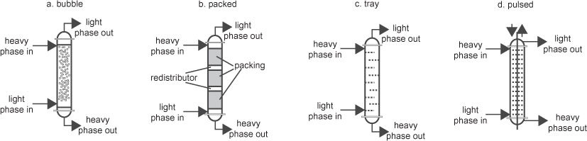
3.4.3 Agitated Columns
Agitated extraction columns involve adding energy via stirrers or similar agitation devices. The York-Scheibel column (Figure 3.46[a]) is designed to simulate a series of mixer-settlers. This type of column has turbine impellers and baffles to simulate a mixer, and the coalescer simulates a settler. The rotating-disk contactor (Figure 3.46[b]) is similar to the York-Scheibel column, except that rotating disks are used to add energy and provide agitation. These columns can have high efficiencies, but that is dependent on the energy input via the shaft. They can be expensive to purchase and to operate, depending on the trade-off between efficiency (column size) and energy input. Other designs include the Oldshue-Rushton (Regents of the University of Michigan, 2014) column and the Kühni column (Koch Modular Process Systems, 2000–2016). The Kühni column can be adapted for changing physical properties within the column and is amenable to scale-up. An advantage of agitated columns is that a large number of theoretical stages is possible, perhaps more than 20 for the Kühni column. The major disadvantage is high cost.
3.4.4 Centrifugal Extractors
Centrifugal extractors contact the two phases continuously by taking advantage of the density difference between the fluids in a centrifugal field. One of the most common centrifugal extractors is a Podbielniak extractor, shown in Figure 3.47. The heavy liquid flows to the outside, while the light liquid flows to the inside. Then both are collected and removed from the device. A single centrifugal extractor can accomplish the separation of five (perhaps a few more) theoretical stages in a single unit. Due to the high centrifugal forces possible, they can handle liquid pairs with small density differences. Centrifugal extractors are expensive to purchase and to operate. Historically, Podbielniak extractors have been used extensively in the pharmaceutical industry where the volume of products are small and highly pure products are required, for example, in the purification of penicillin. A comparison of extraction equipment is in Table 3.10.
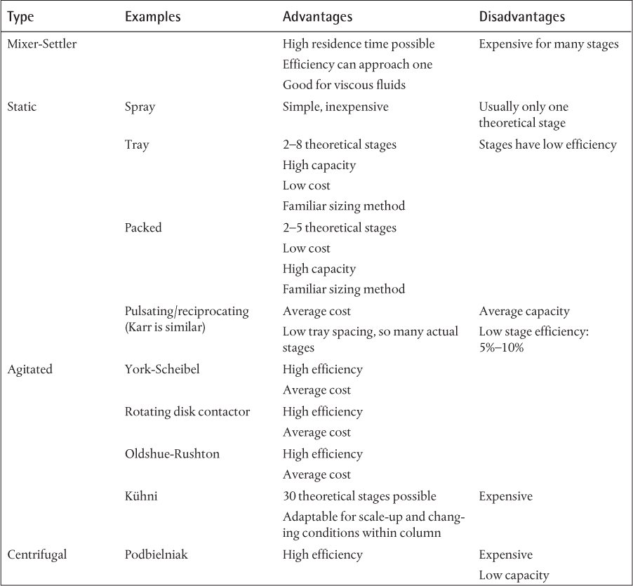
Additional information on extraction equipment is available (Koch and Shiveler, 2015; Koch Modular Processes, 2000–2016).
3.5 Gas Permeation Membrane Separations
Membrane separations include gas permeation, ultrafiltration, reverse osmosis, nanofiltration (such as reverse osmosis, but for organic molecules), and dialysis. Filtration could be considered a membrane separation, although it is often considered to be a fluid mechanics problem, because the key element is flow through the filter cake, which is like a packed bed. While the focus here is on gas permeation, the equipment involved is similar for all membrane separations.
3.5.1 Equipment
Membrane separation equipment generally falls into three general categories. Flat membranes are possible; however, they do not provide much surface area per unit equipment size, so the applications are limited. Spiral-wound membranes create more membrane surface area per volume of equipment. Figure 3.48 illustrates a spiral-wound membrane, and Figure 3.49 illustrates the underlying flow patterns.
With the advent of technology that allows polymers to be spun into hollow fibers, membrane modules that have the appearance of a shell-and-tube heat exchanger were developed. A hollow-fiber module is illustrated in Figure 3.50. The hollow fibers are illustrated in Figure 3.51. Outside diameters are in the 200 to 1000 μm range, and wall thicknesses are in the 50 to 250 μm range. Most of these membranes are asymmetric, meaning that they have multiple layers with different properties. For example, many of these membranes have a support layer with a thin diffusing layer, with the thin diffusing layer on the order of 0.1 μm. For comparison, human hair is in the range of 30 to 100 μm. So, hollow fibers are about an order of magnitude larger than a human hair with a “hole” in the middle that allows the fiber to approximate a tube. Thousands of hollow fibers can be in a single module.
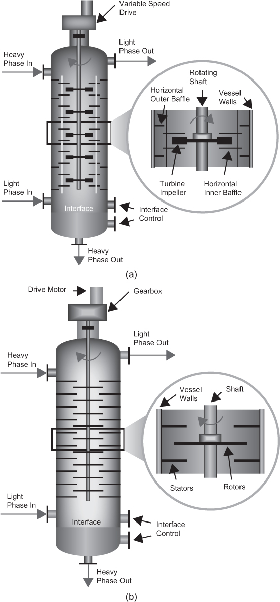
Figure 3.46 (a) York-Scheibel extractor, (b) rotating disk contactor (SCHEIBEL® column courtesy of Koch-Glitsch LP, Wichita, Kansas)

The advantage of hollow-fiber membranes is identical to shell-and-tube heat exchangers, which is that a large amount of surface area/unit volume of equipment is possible. While the module appears to mimic a shell-and-tube heat exchanger, the flow patterns do not. In a shell-and-tube heat exchanger, there are two inlet streams and two outlet streams. In a hollow-fiber module, there is one input and two outputs, with the two outputs being the permeate stream and the less permeable (called retentate) stream. In fact, the most analogous separation to gas permeation from an input-output perspective is a partial vaporization/partial condensation/flash separation (Section 3.2.1).
3.5.2 Models for Gas Permeation Membranes
The simplest possible model for gas permeation membrane equipment is the “well-mixed” model. The validity of this model is discussed later; however, it is useful to understand the concept behind gas permeation. This model is illustrated in Figure 3.52.
The subscripts p and r indicate permeate and retentate, respectively. The variables p and y indicate pressure and mole fraction, respectively, and F indicates molar flowrate. The upstream side is at a higher pressure than the permeate side, which increases the driving force across the membrane. For the simple model, a two-component system is assumed.
A total balance and a balance on the more permeable component are

Figure 3.48 Spiral-wound membrane (Reprinted by permission from Geankoplis [2003])
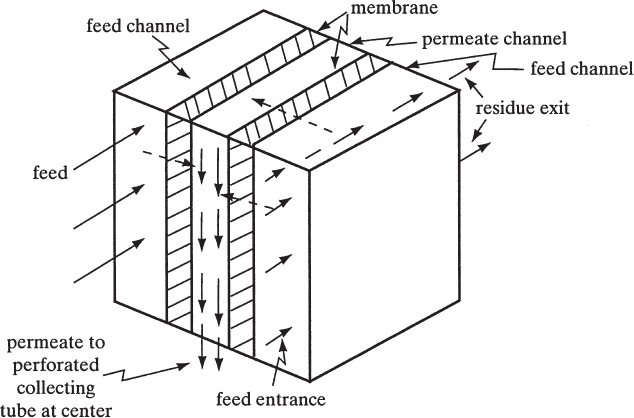
Figure 3.49 Flow patterns in spiral-wound membrane (Reprinted by permission from Geankoplis [2003])
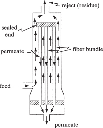
Figure 3.50 Illustration of hollow fiber module (Reprinted by permission from Geankoplis [2003])
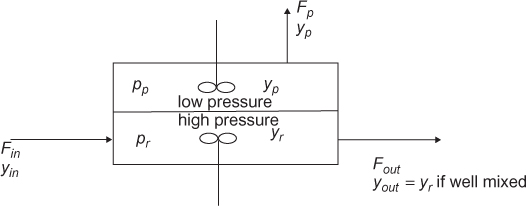
Rearrangement of Equations (3.75) and (3.76) give
where θ = Fp/Fin, which is often called the stage cut. It is a similar term to V/F in the flash-type separations, one outlet flowrate divided by the feed flowrate.
The balances must be combined with rate expressions for transport across the membrane. The rate expressions, assuming ideal gas, are


where PA and PB are the membrane permeabilities of the more permeable component (A) and the less permeable component (B), respectively, and tm is the membrane thickness. Tables of permeabilities are available (Geankoplis, 2003; Wankat, 2017). Taking the ratio of Equations (3.78) and (3.79) yields
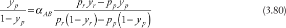
where αAB is the ratio of the permeabilities, PA/PB. Sometimes, the following rearranged form of Equation (3.80) makes calculations easier.

The area, A, can be obtained from either rate expression, Equation (3.78) or (3.79), for a given membrane and thickness, once all flows and mole fractions are known.
Clearly, given the geometry of hollow-fiber membrane modules, the well-mixed assumption is a crude model. Crossflow arrangements are possible, where the feed and retentate are in the middle of the hollow-fiber bundle. Depending on the exact geometry of the equipment, both countercurrent and cocurrent flows are possible, and it is possible to have both in the same piece of equipment. Figure 3.53 illustrates some of these possible flow configurations.
Figure 3.53 Some flow models for gas permeation membranes (Reprinted by permission from Geankoplis [2003])
The mathematical analysis of these models involves differential equations, and they parallel both the development for shell-and-tube heat exchangers and continuous differential separators. Turbulent flow is usually assumed in modeling heat exchangers and packed bed, vapor-liquid separators. However, given the very small diameters involved in hollow-fiber membranes, laminar flow is possible, so the parabolic velocity profile may have to be included. Clearly, these models are far more complex than the well-mixed model, and numerical solutions of the differential equations are often required. A summary of some of these models is available (Geankoplis, 2003).
3.5.3 Practical Issues
Gas permeation is typically used for separations involving noncondensable gases. It is more useful for some separations than for others. As the permeate concentration increases, the permeate flow-rate decreases. Gas permeation equipment can be staged; however, recompression of the permeate is expensive. The upstream side is typically at a higher pressure than the permeate to increase the driving force, as suggested by Equations (3.78) and (3.79). As stated, as the permeate from subsequent stages increases in concentration, the flowrate decreases. Therefore, gas permeation is more useful as a polishing step, that is, removal of dilute contaminants, than as a coarse separation, such as distillation. This suggests that gas permeation may be better suited for purifying the retentate rather than the permeate.
Notation

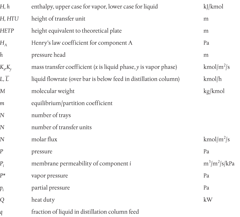
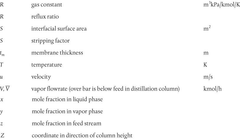
Greek Symbols
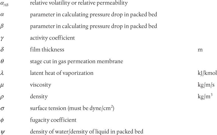
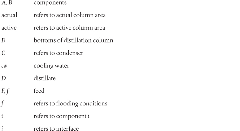
Superscripts

Colburn, A. P. 1939. “A Method of Correlating Forced Convection Heat Transfer Data and a Comparison with Fluid Friction.” Trans AIChE 29: 174.
Couper, J. R., W. R. Penney, J. R. Fair, and S. M. Walas. 2012. Chemical Process Equipment, Selection and Design, 3rd ed. Boston: Elsevier.
Eckert, J. S. 1970. “Selecting the Proper Distillation Column Packing.” Chem Eng Prog 66(3): 39–44.
Fair, J. R., and R. L. Matthews. 1958. “Better Estimate of Entrainment from Bubble-Cap Trays.” Petrol Refin 37(4): 153.
Geankoplis, C. 2003. Transport Processes and Separation Principles, 4th ed. Upper Saddle River, NJ: Prentice Hall.
Hebert, S., and N. Sandford. 2016. “Consider Moving to Fixed Valves.” Chem Engr Prog 112(5): 34–41.
Kister, H. 1992. Distillation Design. New York: McGraw-Hill.
Koch, J., and G. Shiveler. 2015. “Design Principles for Liquid-Liquid Extraction.” Chem Engr Prog 111(11): 22–30.
Koch Modular Processes. 2000–2016. Extraction Column Types. http://modularprocess.com/liquid-liquid-extraction/extraction-column-types.
Kremser, A. 1930. “Theoretical Analysis of Absorption Process.” Natl Petrol News 22(21): 42.
O’Connell, H. E. 1946. “Plate Efficiencies of Fractionating Columns and Absorbers.” Trans Amer Inst Chem Eng 42: 741.
Perry, R. H., and D. W. Green (Eds.). 1997. Perry’s Chemical Engineers’ Handbook, 7th ed. New York: McGraw-Hill, 2-61–2-75.
Pilling, M. 2006. “Design Considerations for High Liquid Rate Tray Applications.” Proceedings of 2006 AIChE Annual Meeting, Paper 264e.
Regents of the University of Michigan. 2014. Encyclopedia of Chemical Engineering Equipment. http://encyclopedia.che.engin.umich.edu/Pages/SeparationsChemical/Extractors/Extractors.html.
Seader, J. D., E. J. Henley, and D. K. Roper. 2011. Separation Process Principles. Chemical and Biochemical Applications, 3rd ed. New York: Wiley.
Souders, M., and G. G. Brown. 1932. “Fundamental Design of High Pressure Equipment Involving
Paraffin Hydrocarbons. IV. Fundamental Design of Absorbing and Stripping Columns for Complex Vapors.” Ind Eng Chem 24: 519–522.
Stichlmair, J. G., and J. R. Fair. 1998. Distillation. Principles and Practice. New York: Wiley.
Treybal, R. E. 1980. Mass Transfer Operations, 3rd ed. New York: McGraw-Hill.
Turton, R., R. C. Bailie, W. B. Whiting, J. A. Shaeiwitz, and D. Bhattacharyya. 2012. Analysis, Synthesis and Design of Chemical Processes, 4th ed. New York: Pearson.
Wankat, P. 2017. Separation Processes. Includes Mass Transfer Analysis, 4th ed. Upper Saddle River, NJ: Prentice Hall.
Problems
Short Answer Problems
1. Sketch a T-xy diagram for an ideal, binary mixture.
a. Illustrate a partial vaporization for a feed of 25 mol% of the more volatile component. Indicate the two phases in equilibrium, the bubble point, and the dew point.
b. Illustrate a partial condensation for a feed of 50 mol% of the more volatile component. Indicate the two phases in equilibrium, the bubble point, and the dew point.
2. Sketch a P-xy diagram for an ideal, binary mixture.
a. Illustrate a flash for a feed of 75 mol% of the more volatile component. Indicate the two phases in equilibrium, the bubble point, and the dew point.
b. Illustrate a partial condensation for a feed of 50 mol% of the more volatile component. Indicate the two phases in equilibrium, the bubble point, and the dew point.
3. What are the physical assumptions of constant molar overflow? What are the consequences? To what types of systems does constant molar overflow typically apply?
4. State three reasons for requiring a high reflux ratio. Illustrate these on a McCabe-Thiele diagram.
5. How does the feed condition (saturated, superheated, subcooled) affect the reflux ratio for a given feed mole fraction? Illustrate the answer on McCabe-Thiele diagrams.
6. What are the limiting cases for reflux ratio? Why are neither of these cases practical?
7. What is the best location for the distillation column feed?
8. What happens if the feed to a distillation column is not at the optimum location? Illustrate this on a McCabe-Thiele diagram.
9. A distillation column requires 18 equilibrium stages that are 40% efficient. It has a partial reboiler.
a. How many trays are in the column if there is a total condenser?
b. How many trays are in the column if there is a partial condenser?
10. Why are some distillation columns run at elevated pressures? State and explain as many reasons as you can.
11. Why are some distillation columns run at vacuum? State and explain as many reasons as you can.
12. The feed to a distillation column is significantly subcooled. What happens on the feed tray? What is the potential effect on column diameter? What is the effect on the reboiler and condenser duties?
13. The feed to a distillation column is significantly superheated. What happens on the feed tray? What is the potential effect on column diameter? What is the effect on the reboiler and condenser duties?
14. Explain the relationship between reflux ratio and the number of equilibrium stages in a distillation column.
15. What is flooding? What is loading? What is weeping?
16. Discuss the advantages and disadvantages of sieve trays versus bubble cap trays.
17. Why might vacuum columns be designed with a larger diameter above the feed compared to below the feed?
18. Does tray spacing have an effect on column diameter? Explain why or why not.
19. The feed to a column is to be saturated liquid. An initial design based on the column conditions below the feed shows that trays above the feed might be weeping. Suggest possible remedies.
20. Discuss the advantages and disadvantages of packed versus tray columns.
21. An existing distillation column is to be scaled up (increase throughput) without changing the distillate and bottom compositions. What happens to the reflux ratio? What problems might arise in the performance of this column?
22. For the distillation column in Problem 3.21, it is suggested to change the pressure of the column. Explain why this might work.
23. For the distillation column in Problems 3.21 and 3.22, how can the pressure in the column be changed?
24. For the distillation column in Problems 3.21, 3.22, and 3.23, someone suggests that the column pressure can be increased by increasing the feed pressure. What is your response? Explain the rationale for your response.
25. The preliminary design of a distillation column shows that it is flooding. If, for some reason, the diameter cannot be changed, suggest two other design modifications that could alleviate this problem, and explain why each works.
26. A colleague gives you a preliminary tray column design. It shows 12-in tray spacing with 8-in weirs. There are 30 actual trays, and the diameter is 5 ft. Comment on all aspects of this design and suggest changes, if necessary.
27. A colleague gives you a preliminary tray column design. It shows 24-in tray spacing with 6-in weirs. There are 60 actual trays and the diameter is 5 ft. Comment on all aspects of this design and suggest changes, if necessary.
28. What is a packing factor, and how does it affect packed column design?
29. What is the absorption (stripping) factor? How does it affect absorber (stripper) design?
30. State three operating conditions that favor absorption (i.e., make absorption easier). Provide a physical explanation for each condition.
31. State three operating conditions that favor stripping (i.e., make stripping easier). Provide a physical explanation for each condition.
32. An absorber is not performing as specified, meaning that the target outlet vapor composition is higher than desired. State as many possible reasons for this that you can identify, and explain why each reason makes physical sense.
33. A stripper is not performing as specified, meaning that the target outlet liquid composition is higher than desired. State as many possible reasons for this that you can identify, and explain why each reason makes physical sense.
34. Comment on the following statement: A transfer unit in a packed column is numerically equivalent to an equilibrium stage in a tray column.
35. What do height of a transfer unit and the number of transfer units indicate?
36. Explain the physical reason why, when the absorption or stripping factor is less than one, increasing the number of stages or increasing packed column height does not increase the recovery of solute.
37. What is the separation basis for distillation? What is the separating agent?
38. What is the separation basis for absorption? What is the separating agent?
39. What is the separation basis for extraction? What is the separating agent?
40. What is the separation basis for leaching? What is the separating agent?
41. What is the separation basis for gas permeation membranes? What is the separating agent?
Problems to Solve
42. For this problem, the feed is 60 mol% dimethyl ether (DME) and 40 mol% methanol. Assume that the equilibrium data provided are correct.
a. A feed of 200 kmol/h is flashed at 5 bar and 50°C. What are the liquid and vapor flowrates and the mole fractions in the vapor and liquid exit streams?
A feed of 200 kmol/h is to be fractionated to give a distillate containing 98 mol% dimethyl ether and a bottoms product containing 98 mol% methanol. The feed is 20% vapor and 80% liquid. There is a total condenser and a partial reboiler.
b. Determine the molar flowrates of the distillate and bottoms.
c. Calculate all internal flows for operation at a reflux ratio of 0.1.
d. In order to use cooling water in the condenser, assume that the DME must condense no lower than 55°C. Estimate the top pressure for this column.
e. In order to use low-pressure steam in the reboiler, the bottom temperature must be no higher than 148°C. Estimate the bottom pressure for this column.
f. Determine the diameter of a sieve tray tower with 18-in tray spacing to operate at 75% of flooding. The active tray area is 85% of the column area. Determine the diameter both above and below the feed. There are six equilibrium stages with the feed on the third stage.
g. Assume that the tray efficiency is 42%. Estimate the maximum weir height for which trays can be designed to meet the pressure specifications.
h. Suppose you determine that the height to diameter ratio for this column exceeds 20, which is usually the maximum recommended value. Suggest at least one design change that would result in a height to diameter ratio smaller than 20. Explain the rationale for your suggestion and its consequences.
i. Determine the diameter of a packed tower to operate at 70% of flooding using 1.5-in, ceramic Berl saddles. Determine the diameter both above and below the feed.
j. Look up the behavior of the DME-methanol system. How would it impact the answers to this problem?

43. Cumene (isopropyl benzene) is manufactured from propylene and benzene. Most of the world’s supply of cumene is directly converted into phenol, which is a raw material for a variety of products such as plasticizers. Acetone is also manufactured as a by-product of phenol manufacture. The separation section of a cumene process consists of a flash, to remove the unreacted propylene, followed by a distillation column to separate the benzene and produce purified cumene as the bottom product.
a. For this problem, consider that the flash contains only propylene and benzene and operates at 3 atm and 100°C. The feed contains 80 mol% benzene and 20 mol% propylene. On a basis of 200 kmol/h feed, determine the flowrates of vapor and liquid leaving the flash.
The feed to the distillation column is 60% liquid at 200 kmol/h containing 48 mol% benzene. It is necessary to produce 99 mol% cumene in the bottom product and 98 mol% benzene in the top product for recycle. The distillation column contains a total condenser and a partial reboiler. The column operates at an average pressure of 3 atm.
b. Determine the flowrates of the distillate and the bottoms.
c. For a reflux ratio of 0.85, calculate all internal flows.
d. Estimate the heat loads (kJ/h) on the condenser and reboiler.
e. Estimate the column efficiency and determine the actual number of trays, the actual number of stages, and the actual feed location. There are 10 equilibrium stages, with feed on Stage 4.
f. Design a sieve tray column for 75% of flooding, with 85% active tray area and with 18-in tray spacing. Specify the column diameter and the actual column height. Ignore the surface tension correction. It is up to you to determine whether to design for the top section or for the bottom section. You should justify your choice.
g. Estimate the pressure drop (kPa) in the column if the trays have 6-in weirs.
h. Design a packed column for 75% of flooding with 2-in, ceramic Raschig rings. It is up to you to determine whether to design for the top section or for the bottom section. You should justify your choice.
i. There is an existing column with the correct number of trays with a 2 m diameter and 85% active area. Will this column work? Explain why or why not. Your answer must be supported with calculations. Could anything be done to make this column work? If so, what are the consequences?
j. The original column is now built and operational, and the feed is 60% liquid. Due to a reactor upset, it is now necessary to accept feed, still 60% liquid, at the same rate but containing 50 mol% benzene, with the remainder cumene. It is still necessary to produce 99 mol% cumene at the same rate from the bottom of this column. You assign your summer intern the job of determining new operating conditions. The answer you get back is to operate at a reflux ratio of 0.75. Will the column operate at these conditions?
Data:
For propylene,
For benzene,
Average column relative volatility = 6
Feed viscosity = 0.3 cP
Benzene density = 800 kg/m3
Cumene density = 700 kg/m3
Benzene heat of vaporization = 3.07 × 10⁴ kJ/kmol
Cumene heat of vaporization = 3.81 × 10⁴ kJ/kmol
Estimated top temperature = 56°C
Estimated bottom temperature = 178°C
Cumene viscosity = 0.3 cP
44. A distillation column is fed 500 kmol/h of an equimolar mixture of pentane and hexane. The feed is saturated liquid. It is necessary to produce outlet streams containing 95 mol% pentane and 99 mol% hexane. The distillation column contains a partial reboiler and a total condenser.
a. Determine the exit flowrates D and B.
b. If the reflux ratio is one, determine all of the internal molar flowrates in the column.
c. Estimate the condenser and reboiler heat loads.
d. In the summer, cooling water is available at 30°C and is returned at 40°C. In the winter, cooling water is available at 25°C and is returned at 35°C. Assuming a 10°C approach in the condenser, based on the cooling water return temperature, determine the seasonal top column pressures.
e. If the column pressure drop is 15 kPa, determine the seasonal bottom column temperatures.
f. There are 15 equilibrium stages, with the feed on stage 5. Determine the diameter of a sieve tray column with 24-in tray spacing for 70% of flooding and an active tray area of 88%. Calculate the diameter for both the top and bottom sections. If the column is designed for the larger diameter, how will the other section perform?
g. Determine the diameter of a packed column with 2-in, ceramic Berl saddles at 70% of flooding. Calculate the diameter for both the top and bottom sections. If the column is designed for the larger diameter, how will the other section perform?
Data:
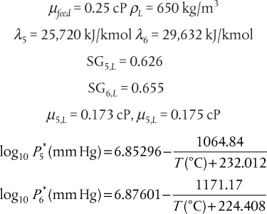
45. For this problem, the feed is 40 mol% heptane and 60 mol% ethylbenzene. A saturated liquid feed of 200 kmol/h is to be fractionated at atmospheric pressure to give a distillate containing 98 mol% heptane and a bottoms product containing 1 mol% heptane.
a. Determine the molar flowrates of distillate and bottoms.
b. Calculate all internal flows for operation at a reflux ratio of 1.5.
c. Estimate the condenser and reboiler duties, in kW.
d. Estimate the top and bottom temperatures, in °C.
e. Design a tray tower with 18-in tray spacing to operate at 75% of flooding. The active tray area is 75%. You should decide whether to design for the top or for the bottom of the column. There are 17 equilibrium stages with the feed on Stage 10.
f. Design a packed tower with 2-in, ceramic INTALOX™ saddles for 70% of flooding. You should decide whether to design for the top or for the bottom of the column.
Vapor pressure data:
For heptane,
For ethylbenzene,
Other data:

46. A feed of 500 kmol/h of methanol and ethanol are to be distilled at 2 bar. The feed is 60 mol% methanol, and the feed is 75% liquid and 25% vapor in equilibrium. The desired outlet compositions are 90 mol% methanol in the distillate and 95 mol% ethanol in the bottoms.
a. Determine the flowrates of the distillate and the bottoms (kmol/h).
b. Calculate all internal flows for a reflux ratio of 3.
c. Determine the diameter of a sieve tray tower with 24-in tray spacing at 70% of flooding with an active tray area of 89%. Design for the top and bottom sections. If the larger diameter is used for the entire column, how will the other section perform? There are 19 equilibrium stages with the feed on Stage 7.
Data:
For methanol,
For ethanol,
Methanol heat of vaporization = 40.5 kJ/mol
Ethanol heat of vaporization = 38.3 kJ/mol
Methanol specific gravity = 0.75
Ethanol specific gravity = 0.75
47. CO2 is to be stripped from water at 20°C and 2 atm using a staged, countercurrent stripper. The liquid flowrate is 100 kmol/h of water with an initial mole fraction of CO2 of 0.00005.
The inlet air stream contains no CO2. A 98.4% removal of CO2 from the water is desired. The Henry’s law constant for CO2 in water at 20°C is 1420 atm.
a. Calculate the outlet mole fraction of CO2 in water.
b. If there are seven equilibrium stages, calculate V and the outlet mole fraction of CO2 in the air.
48. An absorber is designed to treat 40 kmol/h of air containing acetone with a mole fraction of 0.02 and reduce the mole fraction to 0.001. Pure water is the solvent, at a rate of 20 kmol/h. The column temperature is 26.7°C, and the pressure is 1 atm. Raoult’s law may be assumed to apply, and
a. How many equilibrium stages are needed?
b. Assume that a column with five equilibrium stages is built and operational. It is now observed that the outlet mole fraction of acetone in the air is 0.002. Describe and explain at least four possible causes of this situation. Quantify what is happening in the column for each case.
c. Suggest realistic ways to compensate for this problem. An example of a nonrealistic compensation method is to reduce the air feed, which is probably fixed upstream.
d. The column is operating normally, but you are told to expect a 10% increase in air to be treated. How can you change column operation to ensure the desired outlet mole fraction of acetone in air? Be quantitative.
e. The column is operating normally, but you are told to expect an inlet mole fraction of acetone of 0.025. How can you change column operation to ensure the desired outlet mole fraction of acetone in air? Be quantitative.
f. The column is operating normally, but you are told that the outlet mole fraction of acetone must be reduced to 0.00075. How can you change column operation to ensure the desired outlet mole fraction of acetone in air? Be quantitative.
49. Sulfur dioxide (SO2) is removed from a smelter gas (which may be considered to have the properties of pure air) containing 0.80 mol% SO2 by absorption into a solution with the properties of pure water in a countercurrent tower. The exit SO2 concentration in the gas phase must be 0.04 mol%. The tower is designed to operate at exactly 30°C and at 4 bar. At these conditions, the equilibrium relationship is y = 0.1923x, where y is the mole fraction of SO2 in the gas phase, and x is the mole fraction of SO2 in the water phase. The feed rate of gas is 0.36 kmol/s and 1 mole of aqueous solution is used for every 4 moles of feed gas.
a. What is the ratio of the solvent rate to the minimum solvent rate?
b. For a tray tower, determine the number of equilibrium trays required for this separation. Include fractional trays in your answer.
c. Assume the number of equilibrium stages is 6.5. Due to a temporary upset upstream, it is now necessary to treat gas at the higher feed concentration of 1 mol% SO2. If the temperature and pressure must remain constant at 30°C and 4 bar, what do you suggest to accommodate the higher concentration in the feed?
50. An air stream flowing at 1500 kmol/h containing benzene vapor is to be scrubbed using 25 kmol/h of hexadecane (C16H34) as the solvent. The mole fraction of benzene in the inlet gas is 0.010, and the required outlet mole fraction is 0.00050. The hexadecane is being returned to the scrubber from a stripper, so the mole fraction of benzene in the feed hexadecane is 0.00010. The column may be assumed to operate at 150 kPa and 35°C. Raoult’s law may be assumed to define the benzene equilibrium. Dilute solutions may be assumed.
a. How many equilibrium stages are needed? Keep the decimal places.
b. What is the outlet mole fraction of benzene in the hexadecane? What do you conclude about the assumptions made?
c. The column is operational, and the outlet mole fraction of benzene in the air is measured to be 0.0010. You send an operator to check the conditions in the column, and the temperature, pressure, air flowrate, and hexadecane flowrate are all as per design specifications. Suggest two possible causes for the process upset, and provide exact values for the off-spec conditions, assuming that only one condition at a time is off-spec.
d. Determine the diameter of a sieve tray column for an 18-in tray spacing for operation at 75% of flooding. The fraction of active tray area is 0.88.
e. Determine the diameter of a packed column at 75% of flooding with 2-in, ceramic Raschig rings.
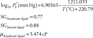
51. A wastewater stream at 35,000 kmol/h containing benzene at a mole fraction of 0.001 is to be stripped with air in a column operating at 2 bar and 25°C. The outlet water must contain no more than 0.00004 mole fraction of benzene. The equilibrium between water and air for benzene at 2 bar and 25°C is y = 150x, where y is the mole fraction of benzene in air and x is the mole fraction of benzene in water. The air used is maintained in a closed loop. Benzene is recovered by condensation from the air stream; therefore, the air entering the stripper contains 0.005 mole fraction of benzene.
a. As part of the design evaluation for this process, it is necessary to determine whether it is feasible to use an existing tray tower for this process. If the tower contains 9 equilibrium stages, and an air rate of 325 kmol/h is the limit set by 80% of flooding, can the tower be used?
b. You observe that there is some flexibility in the operating conditions of the tower in Part (a). Suggest one set of conditions under which the existing tower could be used.
52. When coal is burned to form synthesis gas (syngas), which contains mostly CO, H2, H2S, and CO2, the H2S must be removed. The gas is called syngas because H2 and CO are the building blocks for synthesis of hydrocarbons. One method for removal of H2S is the Selexol™ solvent, in which the H2S is highly soluble. The Selexol solvent is the dimethyl ether of polyethylene glycol and may be assumed to have a molecular weight of 300 kg/kmol, μ = 2.5 × 10⁻³ kg/m s, and ρ = 900 kg/m3.
Consider the removal of H2S only from an otherwise inert mixture of gases; that is, none of the other gases are soluble in the Selexol solvent. The partition coefficient for H2S between gas and solvent is given by the relationship
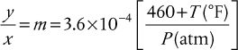
The problem at hand is the removal of H2S from a gas stream with the properties of air, initially containing 2% H2S, so that the exit gas only contains 0.05% H2S. The H2S-rich Selexol solvent is regenerated in a stripper using pure air. The absorber operates at 100 psig (6.8 atm gauge) and 70°F. The stripper operates at 1 atm absolute and 200°F. The stripper reduces the H2S content of the Selexol solvent to 0.5%, which is the feed concentration to the absorber. The gas to be treated is flowing at 1000 kmol/h, and it may be assumed that the Selexol solvent circulates at 30,000 kg/h. In the packed-bed absorber, it is known that HoV = 3.5 m. In the packed-bed stripper, it is known that HoL = 0.25 m. It is proposed to use an existing stripper that is packed with a 5 m high section of 1.5-in, ceramic Raschig rings and has a diameter of 1.8 m.
a. Determine the required absorber height. You may assume that the Colburn method is valid.
b. Determine the exit H2S mole fraction in the Selexol solvent. Comment on this value.
c. For the stripper, determine the amount of air needed.
d. At what percentage of flooding is the stripper operating? Do you recommend operating under these conditions?
e. Determine the pressure drop across the stripper, in kPa.
53. Consider the removal of H2S only from air. The solvent has a molecular weight of 300, μ = 2.5 × 10⁻³ kg/m/s, σ = 30 dyne/cm2, and SG = 0.90. The partition coefficient for H2S between air and solvent is given by the relationship
The problem at hand is the removal of H2S from an air stream initially containing 0.10% H2S, so that the exit gas only contains 0.0050% H2S. The absorber operates at an average pressure of 6 atm and an average temperature of 50°F. The inlet H2S content of the solvent can be assumed to be zero. The gas to be treated is at 200 lbmol/h, and it may be assumed that the solvent circulates at 2100 lb/h.
a. How many equilibrium stages are needed for this separation?
b. There is a problem with the solvent pump, which must be taken off line soon, and the spare pump can only provide solvent at 5 atm at a flowrate no higher than 105% of the original flowrate. Therefore, the feed gas is to be throttled to 5 atm. Since the heat exchangers for this process already uses refrigerated water, 50°F is the lowest possible temperature. You ask two summer interns to evaluate the situation. One says that everything should be okay. The other says that the absorber will not work. Which intern would you hire?
c. What is the diameter of a sieve-tray column for this absorber with 24-in tray spacing for 70% of flooding with an active area of 90% of the total area?
d. If the trays are 20% efficient, is the height/diameter ratio within typical limits? Explain.
e. Estimate the pressure drop in the actual column if there are 6-in weirs.
f. What is the diameter of a packed column for this absorber with 1.5-in, ceramic Berl saddles at 75% of flooding?