
Chapter 3
Databases and Data Acquisition
In Chapter 2, “Understanding Data,” you learned how organizations rely on structured and unstructured data to meet their business needs. The vast majority of transactional systems generate structured data, and we need technology that will help us store all of that data. Databases are the foundational technology that allows us to keep our data organized and easy to retrieve when we need it.
We collect data from many sources to derive insights. For example, a financial analyst wants to understand why some retail outlets are more profitable than others. The analyst might look at the individual records for each store, but that's difficult to do if there are thousands of items and hundreds of stores. Answering the business questions here requires summarizing the data for each store. Databases make it easy to answer this question.
In this chapter, you will examine the two main database categories: relational and nonrelational. You will learn several different approaches for designing databases to store structured data. Building on this foundation, you will learn about common database design practices. You will proceed to dive into the details of working with databases. You will examine tools and techniques that will help you answer questions using data. You will wrap up this chapter by exploring ways to improve the efficiency of how you ask questions. Equipped with this knowledge, you will have a clear understanding of database structure, how data flows between systems, and how to minimize the time needed to get actionable insights.
Exploring Databases
There are many different database options to choose from when an organization needs to store data. While many database products exist, they belong in one of two categories: relational and nonrelational. One of the oldest and most mature databases is the relational database. Relational databases excel at storing and processing structured data. As you discovered in Chapter 2, much of the world's data is unstructured. The need to interact with unstructured data is one of the reasons behind the rise of nonrelational databases.
Although databases fall into two categories, many of the systems we interact with daily produce tabular data. Because tabular data is highly structured, most of this chapter goes deeper into relational databases, their design, and how to use them.
The Relational Model
In 1969, IBM's Edgar F. Codd developed the relational model for database management. The relational model builds on the concept of tabular data. In the relational model, an entity contains data for a single subject. When creating an IT system, you need to consider all the entities required to make your system work. You can think of entities as nouns because they usually correspond to people, places, and things.
Imagine a veterinary clinic that has to store data about the animals it treats and the people who own those animals. The clinic needs one entity for data about animals and a separate entity for data about people to accomplish this goal. Figure 3.1 shows the structure of the Animal and Person entities.
An entity instance identifies a specific example of an entity. Considering the Animal entity in Figure 3.1, an entity instance is a particular animal. Looking at Table 3.1, all of the information about Jack represents an entity instance.
TABLE 3.1 Animal data
| Animal_ID | Animal_Name | Animal_Type | Breed_Name | Date_of_Birth | Height (inches) | Weight (pounds) |
|---|---|---|---|---|---|---|
| 1 | Jack | Dog | Corgi | 3/2/2018 | 10 | 26.3 |
| 2 | Viking | Dog | Husky | 5/8/2017 | 24 | 58 |
| 3 | Hazel | Dog | Labradoodle | 7/3/2016 | 23 | 61 |
| 4 | Schooner | Dog | Labrador Retriever | 8/14/2019 | 24.3 | 73.4 |
| 5 | Skippy | Dog | Weimaraner | 10/3/2018 | 26.3 | 63.5 |
| 6 | Alexander | Cat | American Shorthair | 10/4/2017 | 9.3 | 10.4 |
For both entities in Figure 3.1, the bolded word in the header is the entity's name. For example, suppose you want to know where to look for data about a specific person. The Person entity in Figure 3.1 is a clear choice since it stores data about people.
Understanding that the header corresponds to the name of an entity, look at the rows of the Person entity. Each row represents an individual attribute associated with a person. Suppose you want to enhance the Person entity to accommodate a mobile phone number. You would just edit the Person entity to include a mobile phone attribute.
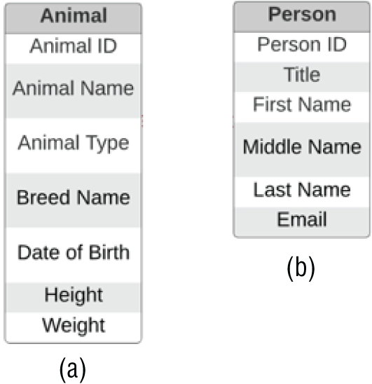
FIGURE 3.1 The (a) Animal entity and (b) Person entity in a veterinary database
Each of these entities becomes a separate table in the database, with a column for each attribute. Each row represents an instance of the entity. The power of the relational model is that it also allows us to describe how entities connect, or relate, to each other. The veterinary clinic needs to associate animals with people. Animals do not have email addresses, cannot schedule appointments, and cannot pay for services. Their owners, on the other hand, do all of these things. There's a relationship between animals and people, and we can include this relationship in our database design, as shown in Figure 3.2.

FIGURE 3.2 Relationship connecting Animal and Person
The entity relationship diagram (ERD) is a visual artifact of the data modeling process. It shows the connection between related entities. The line in Figure 3.2 illustrates that a relationship exists between the Animal and Pet entities. A relationship is a connection between entities. The symbols adjacent to an entity describe the relationship.
Cardinality refers to the relationship between two entities, showing how many instances of one entity relate to instances in another entity. You specify cardinality in an ERD with various line endings. The first component of the terminator indicates whether the relationship between two entities is optional or required. The second component indicates whether an entity instance in the first table is associated with a single entity instance in the related table or if an association can exist with multiple entity instances. Figure 3.3 illustrates the possible combinations for representing relationships.
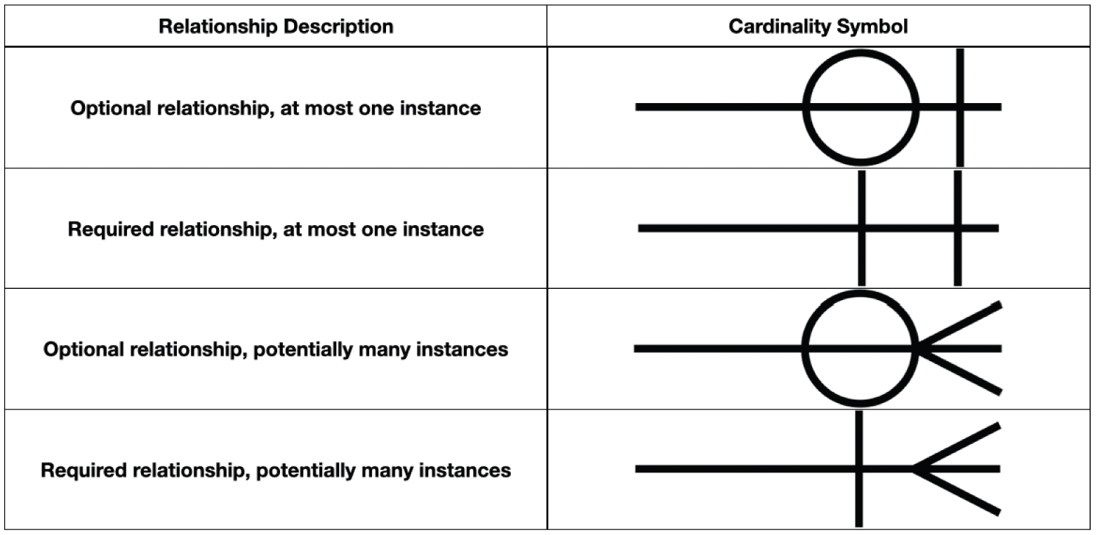
FIGURE 3.3 ERD line endings
With an understanding of ERD line endings, let's apply it to Figure 3.2. Reading the diagram aloud from left to right, you say, “An individual animal belongs to at least one and possibly many people.” Reading from right to left sounds like, “A specific person has at least one and possibly many animals.”
A unary relationship is when an entity has a connection with itself. For example, Figure 3.4 illustrates a unary relationship where a single manager has multiple employees.

FIGURE 3.4 Unary relationship
A binary relationship connects two entities, as seen in Figure 3.2. A ternary relationship connects three entities. For example, you might use a ticket entity to connect a venue, a performing artist, and a price.
Binary relationships are the most common and easy to explore, whereas unary and ternary are comparatively complex and rare.
As you think about a database that would support an actual veterinary clinic, you're probably realizing that it would need to store more information than we've already discussed. For example, we'd need to store addresses, appointments, medications, and procedures. Database designers would continue to add entities and relationships to the diagram until it meets all of the veterinary clinic's business needs, such as the one shown in Figure 3.5.

FIGURE 3.5 Entity relationship diagram
Apart from being a helpful picture, the entity relationship diagram also serves as a relational database's blueprint. The ability to read ERDs helps you understand the structure of a relational database. ERDs are particularly useful when formulating how to retrieve information from the database that is spread across multiple tables because the diagrams allow you to visualize the connections between entities.
Relational Databases
Relational databases are pieces of software that let you make an operational system out of an ERD. You start with a relational model and create a physical design. Relational entities correspond to database tables, and entity attributes correspond to table columns. When creating a database table, the ordering of columns does not matter because you can specify the column order when retrieving data from a table. When an attribute becomes a column, you assign it a data type. Completing all of this work results in a diagram known as a schema. You can think of a schema as an ERD with the additional details needed to create a database. For example, the relational model in Figure 3.2 becomes the schema in Figure 3.6.
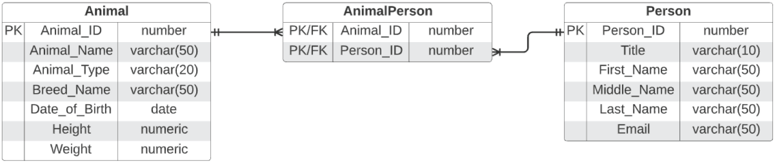
FIGURE 3.6 Database schema
Note that the two entities in Figure 3.2 become three tables in Figure 3.6. The new AnimalPerson table is necessary because you need to resolve a many-to-many relationship with an associative table. An associative table is both a table and a relationship. Recall that an animal can belong to more than one person, and a person can have more than one animal. An associative table lets you identify the relationship between a specific animal and a particular person with a minimum amount of data duplication. Let's examine the tables and their data in more detail to see the Animal, AnimalPerson, and Person tables in action.
With the schema design complete, you can build the tables. Once you have the tables, you can load them with data. Table 3.1 shows what the Animal entity from Figure 3.1 looks like with data.
Similarly, the Person entity from Figure 3.1 corresponds to Table 3.2. The first column in both Table 3.1 and Table 3.2 is an identifier with a numeric data type. In both cases, these identifier columns (Animal_ID and Person_ID) are the primary key for the table. A primary key is one or more attributes that uniquely identify a specific row in a table. It is best to use a synthetic primary key, which is simply an attribute whose only purpose is to contain unique values for each row in the table. In Table 3.1, Animal_ID is a synthetic primary key, and the number 3 is arbitrarily assigned to Hazel. The number 3 has no meaning beyond its ability to uniquely identify a row. Nothing about Hazel's data changes if her Animal_ID was 7 instead of 3. Taking another look at Figure 3.6, note how PK denotes the primary key for the Animal, AnimalPerson, and Person tables.
Note that within a given table, the actual sequencing of the rows does not matter. For example, you might want to retrieve data from Table 3.2 alphabetically by first or last name. Using SQL, you can easily specify the order in which you want to bring data back from a table.
TABLE 3.2 Person Data
| Person_ID | Title | First_Name | Middle_Name | Last_Name | |
|---|---|---|---|---|---|
| 10000 | Mr | Paul | Tupy | [email protected] | |
| 10001 | Ms | Emma | M | Snyder | [email protected] |
| 10002 | Ms | Giustina | Marguerite | Rossi | [email protected] |
| 10003 | Mr | Giacomo | Paolo | Mangione | [email protected] |
| 10004 | Mrs | Eleonora | B | Mangione | [email protected] |
| 10005 | Ms | Leila | Abir | Abboud | [email protected] |
| 10006 | Mr | Chris | Thomas | Bregande | [email protected] |
You can imagine the data in Tables 3.1 and 3.2 existing as separate tabs in a spreadsheet. Suppose both Hazel and Alexander belong to the Mangione family. There is nothing in the data that connects an animal to a person. To link the two tables, you need a foreign key. A foreign key is one or more columns in one table that points to corresponding columns in a related table. Frequently, a foreign key references another table's primary key. Looking at the AnimalPerson table in Figure 3.6, FK denotes a foreign key. The Person_ID in the AnimalPerson table points to the Person_ID in the Person table. You can't put a row in the AnimalPerson table if the Person_ID doesn't exist in the Person table. Similarly, you can't use an Animal_ID in AnimalPerson if it doesn't exist in the Animal table.
Every row in a relational database must be unique. In Table 3.1, each row contains data about a specific animal, whereas each row in Table 3.2 refers to a particular person. Since the Mangione family has multiple animals, we need an associative table to describe the relationship between Animal and Person. Table 3.3 shows data from the AnimalPerson table in Figure 3.6.
TABLE 3.3 AnimalPerson table
| Animal_ID | Person_ID |
|---|---|
| 3 | 10003 |
| 3 | 10004 |
| 6 | 10003 |
| 6 | 10004 |
Suppose you want to send an email reminder about an upcoming appointment for a pet. Figure 3.7 shows an email template with placeholder values.

FIGURE 3.7 Email template
To populate the email template, you need the person's title, last name, and email address from Table 3.2 and the corresponding pet's name and animal type from Table 3.1. To pull data from a relational database table, you perform a query. You compose queries using a programming language called Structured Query Language (SQL).
Your query needs to perform a database join to retrieve the data to substitute in the email reminder. A join uses data values from one table to retrieve associated data in another table, typically using a foreign key.
The first row in Table 3.3 represents the relationship between Mr. Mangione and Hazel. To send Mr. Mangione an email, you take 10003, the value for Person_ID in the first row of Table 3.3, and join it to Table 3.2. Using 10003, you retrieve Mr. Mangione's title, last name, and email address. To retrieve Hazel's information, you perform a similar join. You get 3 for Animal_ID from Table 3.3 and look up Hazel's information in Table 3.1. The result is the email that gets sent, shown in Figure 3.8. Note that if you send an email for each row in Table 3.3, both Mr. and Mrs. Mangione get emails about Hazel the Dog and Alexander the Cat.
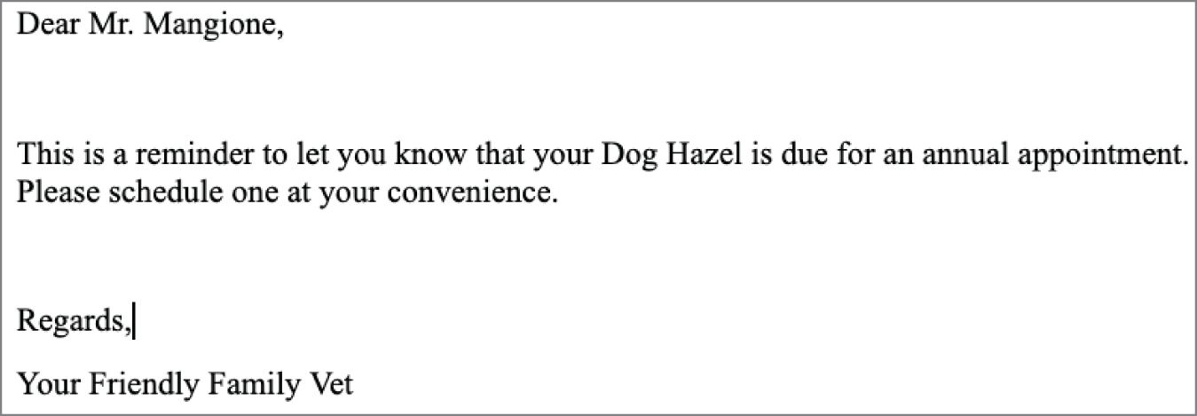
FIGURE 3.8 Reminder appointment email
Foreign keys enforce referential integrity, or how consistent the data is in related tables. Consider Figure 3.9, which shows why referential integrity is crucial to enforcing data quality. Suppose you try to add a row to the middle table, specifying 6 for the Animal_ID and 99999 as the Person_ID. The foreign key on Animal_ID checks the table to the left to ensure a row exists with the Animal_ID of 6. The new record passes this check because there is a record with Animal_ID 6 for the cat named Alexander. When a similar check happens on Person_ID, there is no row corresponding to the Person_ID 99999 in the table on the right. Therefore, adding the new row fails, and the relationship between the tables is maintained.
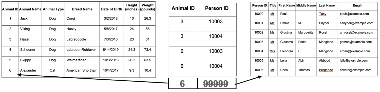
FIGURE 3.9 Referential integrity illustration
In Table 3.3, the Animal_ID column is a foreign key that points to the Animal_ID primary key in Table 3.1. Looking at the first data row in Table 3.3, Animal_ID 3 refers to Hazel. Similarly, the Person_ID column points to the Person_ID column in Table 3.2, with 10003 identifying Giacomo Mangione. The combination of both Animal_ID and Person_ID is what makes each row in Table 3.3 unique. Taken together, Animal_ID and Person_ID represent a composite primary key. As the name implies, a composite primary key is a primary key with more than one column. While Figure 3.2 describes a relational model, Figure 3.6 shows modifications necessary to create tables for storing data.
Relational databases are complicated to operate at scale. A database administrator (DBA) is a highly trained person who understands how database software interacts with computer hardware. A DBA looks after how the database uses the underlying storage, memory, and processor resources assigned to the database. A DBA also looks for processes that are slowing the entire database down.
Nonrelational Databases
A nonrelational database does not have a predefined structure based on tabular data. The result is a highly flexible approach to storing data. However, the data types available in relational databases are absent. As a result, you need to know more about the data itself to interact with it. Data validation happens in code, as opposed to being done in the database. Examples of nonrelational databases include key-value, document, column family, and graph.
Key-Value
A key-value database is one of the simplest ways of storing data. Data is stored as a collection of keys and their corresponding values. A key must be globally unique across the entire database. The use of keys differs from a relational database, where a given key identifies an individual row in a specific table. There are no structural limits on the values of a key. A key can be a sequence of numbers, alphanumeric strings, or some other combination of values.
The data that corresponds with a key can be any structured or unstructured data type. Since there are no underlying table structures and few limitations on the data that can be stored, operating a key-value database is much simpler than a relational database. It also can scale to accommodate many simultaneous requests without impacting performance. However, since the values can contain multiple data types, the only way to search is to have the key.
One reason for choosing a key-value database is when you have lots of data and can search by a key's value. Imagine an online music streaming service. The key is the name of a song, and the value is the digital audio file containing the song itself. When a person wants to listen to music, they search for the name of the song. With a known key, the application quickly retrieves the song and starts streaming it to the user.
Document
A document database is similar to a key-value database, with additional restrictions. In a key-value database, the value can contain anything. With a document database, the value is restricted to a specific structured format. For example, Figure 3.12 is an example of using JSON as the document format.
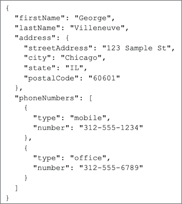
FIGURE 3.12 JSON person data
With a known, structured format, document databases have additional flexibility beyond what is possible with key-value. While searching with a known document key yields the fastest results, searching using a field within the document is possible. Suppose you are storing social network profiles. The document key is the profile name. The document itself is a JSON object containing details about the person, as Figure 3.6 shows. With a document database, it is possible to retrieve all profiles that match a specific zip code. This searching ability is possible because the database understands the document's structure and can search based on data within the document.
Column Family
Column-family databases use an index to identify data in groups of related columns. A relational database stores the data in Table 3.2 in a single table, where each row contains the Person_ID, Title, First_Name, Middle_Name, Last_Name, and Email columns. In a column-family database, the Person_ID becomes the index, while the other columns are stored independently. This design facilitates distributing data across multiple machines, which enables handling massive amounts of data. The ability to handle large data volumes is due to the technical implementation details of how these databases organize and store. From a design standpoint, column-family databases optimize performance when you need to examine the contents of a column across many rows.
The main reason for choosing a column-family database is its ability to scale. Suppose you need to analyze U.S. stock transactions over time. With daily trade volumes of over 6 billion records, processing that amount of data on a single database server is not feasible. It is in situations like this where column-family databases shine.
Graph
Graph databases specialize in exploring relationships between pieces of data. Consider Figure 3.6, which shows the tables required to indicate which animals belong to which people. Figure 3.13 illustrates how a graph models data from Tables 3.1 and 3.2. Each animal and person represents a node in the graph. Each node can have multiple properties. Properties store specific attributes for an individual node. The arrow connecting nodes represents a relationship.
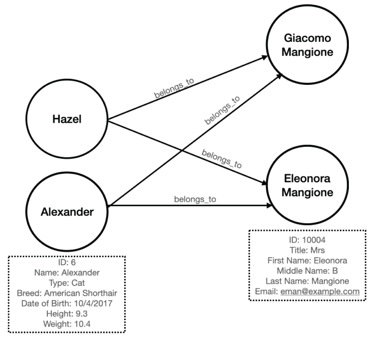
FIGURE 3.13 Data in a graph
Relational models focus on mapping the relationships between entities. Graph models map relationships between actual pieces of data. In Figure 3.6, you have to use three tables to represent the same data in Figure 3.13. Since fewer objects are involved, graphs allow you to follow very quickly.
Graphs are an optimal choice if you need to create a recommendation engine, as graphs excel at exploring relationships between data. For example, when you search for a product on an e-commerce website, the results are frequently accompanied by a collection of related items. Understanding the connection between products is a challenge that graphs solve with ease.
Database Use Cases
Different business needs require different database designs. While all databases store data, the database's structure needs to match its intended purpose. Business requirements impact the design of individual tables and how they are interconnected. Transactional and reporting systems need different implementation approaches to serve the people who use them efficiently. Databases tend to support two major categories of data processing: Online Transactional Processing (OLTP) and Online Analytical Processing (OLAP).
Online Transactional Processing
OLTP systems handle the transactions we encounter every day. Example transactions include booking a flight reservation, ordering something online, or executing a stock trade. While the number of transactions a system handles on a given day can be very high, individual transactions process small amounts of data. OLTP systems balance the ability to write and read data efficiently.
Based on the data in Table 3.1, Table 3.2, and Table 3.3, suppose Giacomo Mangione wants to book an annual visit appointment for his cat Alexander. Suppose both Giacomo and Alexander already exist in the database that supports the appointment system, as shown in Figure 3.14.
To book an appointment, Giacomo logs in to the vet clinic's website. When Giacomo logs in, the system retrieves his information from the Person table. Using the Animal_IDs corresponding to his Person_ID in the AnimalPerson table, the system displays a list of Giacomo's animals. Selecting Alexander from the list, Giacomo specifies a date and time of his choosing. Giacomo's input represents all the data necessary to create an appointment record, which Table 3.4 illustrates.
TABLE 3.4 Appointment booking
| Appt_ID | AnmlPers_ID | Date | Time |
|---|---|---|---|
| 53 | 10003 | 5/5/2022 | 13:00 |

FIGURE 3.14 Vet clinic transactional schema
In Table 3.4, the AnmlPers_ID identifies Giacomo and Alexander. The Appt_ID is a system-generated synthetic key while Giacomo supplies the Date and Time. To retrieve the rest of the details about the person and the animal, you need to join the tables together using the foreign key to primary key relationship.
For this appointment, Alexander is due for a complete blood count and blood chemistry panel. The details about each procedure are in the Procedure table in Figure 3.14. The AppointmentProcedure table provides the link between a given appointment and all of the procedures performed during that appointment.
Online Analytical Processing
OLAP systems focus on the ability of organizations to analyze data. While OLAP and OLTP databases can both use relational database technology, their structures are fundamentally different. OLTP databases need to balance transactional read and write performance, resulting in a highly normalized design. Typically, OLTP databases are in 3NF.
On the other hand, databases that power OLAP systems have a denormalized design. Instead of having data distributed across multiple tables, denormalization results in wider tables than those found in an OLTP database. It is more efficient for analytical queries to read large amounts of data for a single table instead of incurring the cost of joining multiple tables together.
Imagine you want to create a summary of the clinic's interaction history with a family's pets, as shown in Figure 3.18. Using the normalized OLTP database from Figure 3.14, you need to retrieve data from the Procedure, AppointmentProcedure, Appointment, AnimalPerson, and Animal tables. The greater the number of joins, the more complex the query. The more complex the query, the longer it takes to retrieve results.
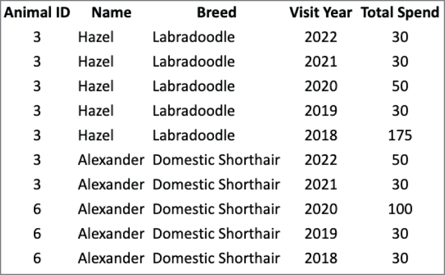
FIGURE 3.18 Yearly spend by animal
Consider the table in Figure 3.19, whose structure easily supports the data in Figure 3.18. It is possible to create the summary in Figure 3.18 using the OLTP database from Figure 3.14. However, the CostSummary table in Figure 3.19 greatly simplifies that operation.

FIGURE 3.19 CostSummary table
Schema Concepts
The design of a database schema depends on the purpose it serves. Transactional systems require highly normalized databases, whereas a denormalized design is more appropriate for analytical systems. A data warehouse is a database that aggregates data from many transactional systems for analytical purposes. Transactional data may come from systems that power the human resources, sales, marketing, and product divisions. A data warehouse facilitates analytics across the entire company.
A data mart is a subset of a data warehouse. Data warehouses serve the entire organization, whereas data marts focus on the needs of a particular department within the organization. For example, suppose an organization wants to do analytics on their employees to understand retention and career evolution trends. To satisfy that use case, you can create a data mart focusing on the human resources subject area from the data warehouse.
A data lake stores raw data in its native format instead of conforming to a relational database structure. Using a data lake is more complex than a data warehouse or data mart, as it requires additional knowledge about the raw data to make it analytically useful. Relational databases enforce a structure that encapsulates business rules and business logic, both of which are missing in a data lake.
For data warehouses and data marts, several design patterns exist for modeling data. It is crucial to realize that the structure of a database schema impacts analytical efficiency, particularly as the volume of data grows. In addition to a schema's design, it is vital to consider the life cycle. Life-cycle considerations include where data comes from, how frequently it changes, and how long it needs to persist.
Star
The star schema design to facilitate analytical processing gets its name from what the schema looks like when looking at its entity relationship diagram, as Figure 3.20 illustrates. Star schemas are denormalized to improve read performance over large datasets.

FIGURE 3.20 Star schema example
At the center of the star is a fact table. Fact tables chiefly store numerical facts about a business. In Figure 3.20, the schema design centers on reporting on the cost and profitability of procedures. Qualitative data, including names, addresses, and descriptions, is stored in a series of dimension tables that connect to the main fact table.
Consider Figure 3.20, which has the Procedure_Facts table at the center of the star. This table makes it straightforward to calculate overall profitability. If you want to explore profitability for cats, you need to join the Procedure_Facts table to the Animal_Dimension. Similarly, you can join in the Procedure_Dimension table to understand profitability by procedure name. The Time_Dimension is unique in that it makes it easy to look at profitability by day of week, quarter, month, or any other time-related attribute.
With a fact table surrounded by dimension tables, the queries to answer questions are simple to write and understand. Suppose you want to understand the aggregate cost of all procedures performed on dogs. In Figure 3.21, the OLTP Query shows how to answer that question using the transactional schema from Figure 3.14. The Star Schema Query provides the same answer, using the schema in Figure 3.20.
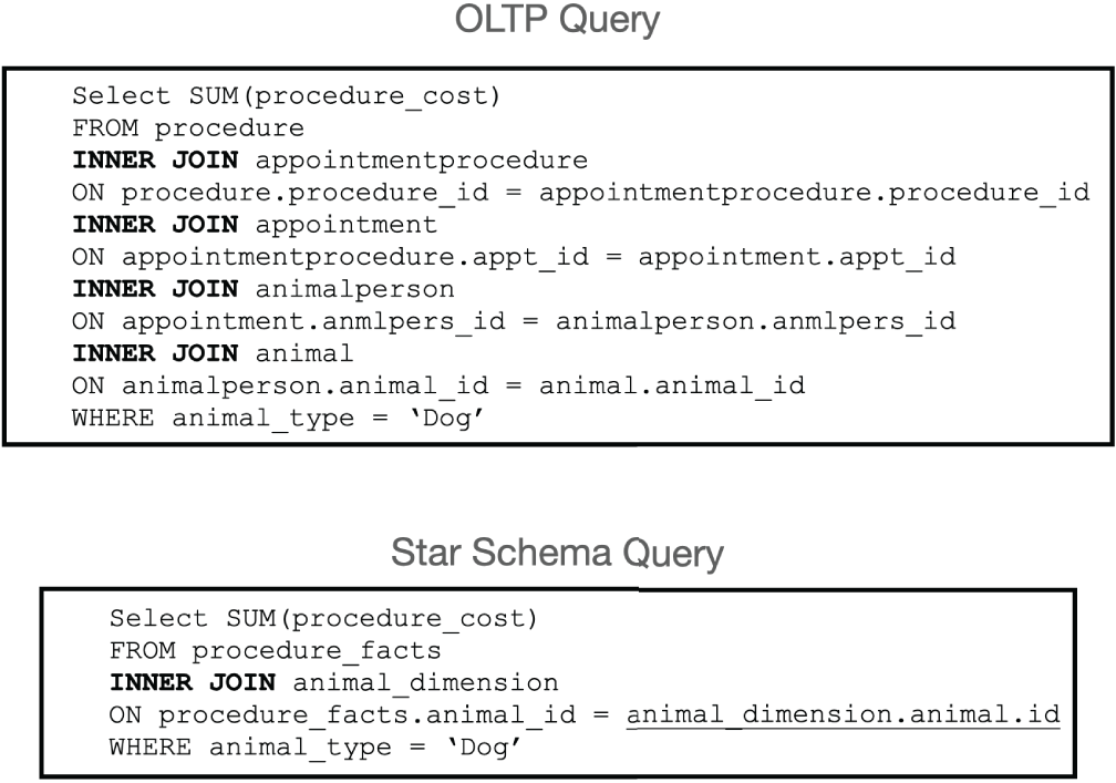
FIGURE 3.21 OLTP and OLAP query example
Even if you have never seen SQL before, you can appreciate that the four INNER JOIN statements in the OLTP Query indicate that you need five tables to get the result. In contrast, the single INNER JOIN in the Star Schema Query requires two tables. Now imagine that you want to get procedure cost by animal type and zip code. Crafting that query using the schema in Figure 3.14 requires you to bring in the Person, PersonAddress, and Address tables. Using the star schema from Figure 3.20, you only need to add the Person_Dimension table.
When data moves from an OLTP design into a star schema, there is a significant amount of data duplication. As such, a star schema consumes more space than its associated OLTP design to store the same data. These additional resource needs are one of the factors that makes data warehouses expensive to operate.
Snowflake
Another design pattern for data warehousing is the snowflake schema. As its name implies, the schema diagram looks like a snowflake. Snowflake and star schemas are conceptually similar in that they both have a central fact table surrounded by dimensions. Where the approaches differ is in the handling of dimensions. With a star, the dimension tables connect directly to the fact table. With a snowflake, dimensions have subcategories, which gives the snowflake design its shape. A snowflake schema is less denormalized than the star schema.
Recall that in a star schema, dimensions are one join away from the fact table. With a snowflake schema, you may need more than one join to get the data you are looking for. Consider the Day, Quarter, and State lookup tables in Figure 3.22. The data for State_Description is in the State table. In Figure 3.20, State_Description exists in the Person_Dimension.

FIGURE 3.22 Snowflake example
Recall that as the number of tables in a schema grows, queries become more complicated. For example, suppose you want to get procedure cost on a quarter-by-quarter basis and include Quarter_Name in the output. Using a star schema, you need two tables to answer this question. With the snowflake from Figure 3.22, you need three.
A snowflake schema query is more complex than the equivalent query in a star schema. Part of the trade-off is that a snowflake schema requires less storage space than a star schema. Consider where State_Description exists in Figure 3.20 and Figure 3.22. When State_Description is in a separate lookup table, it also consumes much less storage space. Imagine that there are 1 billion rows in the Person_Dimension table. In a star schema, the State_Description is stored 1 billion times. With a snowflake schema, you only end up storing State_Description 50 times—once for each of the 50 U.S. states.
Data warehouses often use snowflake schemas, since many different systems supply data to the warehouse. Data marts are comparatively less complicated, because they represent a single data subject area. As such, data marts frequently use a star-schema approach.
Dimensionality
Dimensionality refers to the number of attributes a table has. The greater the number of attributes, the higher the dimensionality. A dimension table provides additional context around data in fact tables. For example, consider the Person_Dimension table in Figure 3.22, which contains details about people. If you need additional data about people, add columns to Person_Dimension.
It is crucial to understand the types of questions an analyst will need to answer when designing dimension tables. For example, a vice president of sales may want to examine profitability by geographical region and time of year. They may want to zoom in and look at product sales by day to gauge the effectiveness of a marketing campaign. They may also want to better understand trends by product and product family.
One dimension you will frequently encounter is time. It is necessary to answer questions about when something happened or when something was true. For example, to understand historical profitability, you need to keep track of pricing at the product level over time. One way to accomplish this is to add a start and end date to each product's price.
Consider Table 3.5, reflecting the price history for a 17 mm socket in a product dimension table. This table illustrates one approach to handling time. The last price change went into effect on January 1, 2021. The value for this date goes in the End_Date column for the $7.39 price and the Start_Date column for the $6.29 price. With this approach, it is easy to identify a 17 mm socket price on any given day after its original on-sale date.
TABLE 3.5 Product dimension
| Product_ID | Product_Name | Price | Start_Date | End_Date |
|---|---|---|---|---|
| 53 | 17 mm socket | 5.48 | 1993-01-01 00:00:00 | 2003-01-01 00:00:00 |
| 53 | 17 mm socket | 5.89 | 2003-01-01 00:00:00 | 2013-01-01 00:00:00 |
| 53 | 17 mm socket | 5.99 | 2013-01-01 00:00:00 | 2020-05-03 00:00:00 |
| 53 | 17 mm socket | 6.23 | 2020-05-03 00:00:00 | 2020-05-31 00:00:00 |
| 53 | 17 mm socket | 8.59 | 2020-05-31 00:00:00 | 2020-10-31 00:00:00 |
| 53 | 17 mm socket | 7.39 | 2020-10-31 00:00:00 | 2021-01-01 00:00:00 |
| 53 | 17 mm socket | 6.29 | 2021-01-01 00:00:00 | 9999-12-31 23:59:59 |
Imagine a time-specific dimension that allows grouping by various time increments, including the day of the year, day of the week, month, and quarter. Using time stamp data types for both the Start_Date and End_Date columns in Table 3.5 makes it easy to calculate the average price for all sockets regardless of the level of time detail.
One of the criteria to consider is how quickly a dimension changes over time. Consider a geographic dimension table containing the 50 U.S. states. Ever since Hawaii became the 50th state in 1959, the number of states has remained constant. Looking forward, it is unlikely that additional states will enter the union with great frequency. In this context, geography is an example of a slowly changing dimension. However, other geographic attributes change more quickly. For example, a person's street address is more likely to change than the number of states in the United States.
Regardless of the speed at which a dimension changes, you need to handle both current and historical data.
Handling Dimensionality
There are multiple ways to design dimensions. Table 3.5 illustrates the start and end date approach. An understanding of this method is required to write a query to retrieve the current price. Another method extends the snowflake approach to modeling dimensions. You have a product dimension for the current price and a product history table for maintaining price history. One advantage of this approach is that it is easy to retrieve the current price while maintaining access to historical information.
Another approach is to use an indicator flag for the current price. This approach requires another column, as shown in Table 3.6. The indicator flag method keeps all pricing data in a single place. It also simplifies the query structure to get the current price. Instead of doing date math, you look for the price where the Current flag equals “Y.”
TABLE 3.6 Current flag
| Product_ID | Product_Name | Price | Start_Date | End_Date | Current |
|---|---|---|---|---|---|
| 53 | 17 mm socket | 8.59 | 2020-05-31 00:00:00 | 2020-10-31 00:00:00 | N |
| 53 | 17 mm socket | 7.39 | 2020-10-31 00:00:00 | 2021-01-01 00:00:00 | N |
| 53 | 17 mm socket | 6.29 | 2021-01-01 00:00:00 | 9999-12-31 23:59:59 | Y |
It is also possible to use the effective date approach to handling price changes. Consider Table 3.7, which illustrates this approach. In the table, each row has the date on which the given price goes into effect. The assumption is that the price stays in effect until there is a price change, at which point a new row is added to the table.
TABLE 3.7 Effective date
| Product_ID | Product_Name | Price | Effective_Date |
|---|---|---|---|
| 53 | 17 mm socket | 8.59 | 2020-05-31 00:00:00 |
| 53 | 17 mm socket | 7.39 | 2020-10-31 00:00:00 |
| 53 | 17 mm socket | 6.29 | 2021-01-01 00:00:00 |
There is additional complexity with the effective date approach because queries have to perform date math to determine the price. Looking at the table, the price of 8.59 went into effect on May 31, 2020. The price changes on October 31, 2020. To retrieve the price on October 3, 2020, we know that October 3 falls after May 31 and before October 31. As such, the price on May 31 is current on October 3. While it is possible to code this logic in SQL, it complicates the queries.
Data Acquisition Concepts
To perform analytics, you need data. Data can come from internal systems you operate, or you can obtain it from third-party sources. Regardless of where data originates, you need to get data before analyzing it to derive additional value. In this section, we explore methods for integrating data from systems you own. We also explore strategies for collecting data from external systems.
Integration
Data from transactional systems flow into data warehouses and data marts for analysis. Recall that OLTP and OLAP databases have different internal structures. You need to retrieve, reshape, and insert data to move data between operational and analytical environments. You can use a variety of methods to transfer data efficiently and effectively.
One approach is known as extract, transform, and load (ETL). As the name implies, this method consists of three phases.
- Extract: In the first phase, you extract data from the source system and place it in a staging area. The goal of the extract phase is to move data from a relational database into a flat file as quickly as possible.
- Transform: The second phase transforms the data. The goal is to reformat the data from its transactional structure to the data warehouse's analytical design.
- Load: The purpose of the load phase is to ensure data gets into the analytical system as quickly as possible.
Extract, load, and transform (ELT) is a variant of ETL. With ELT, data is extracted from a source database and loaded directly into the data warehouse. Once the extract and load phases are complete, the transformation phase gets under way. One key difference between ETL and ELT is the technical component performing the transformation. With ETL, the data transformation takes place external to a relational database, using a programming language like Python. ELT uses SQL and the power of a relational database to reformat the data.
ELT has an advantage in the speed with which data moves from the operational to the analytical database. Suppose you need to get massive amounts of transactional data into an analytical environment as quickly as possible. In that case, ELT is a good choice, especially at scale when the data warehouse has a lot of capacity. Whether you choose ETL or ELT is a function of organizational need, staff capabilities, and technical strategy.
An initial load occurs the first time data is put into a data warehouse. After that initial load, each additional load is a delta load, also known as an incremental load. A delta load only moves changes between systems. Figure 3.23 illustrates a data warehouse that launches in January and uses a monthly delta load cycle. The initial load happens right before the data warehouse becomes available for use. All of the transactional data from January becomes the delta load that initiates on the first of February. Figure 3.23 illustrates a monthly delta-load approach that continues throughout the year.
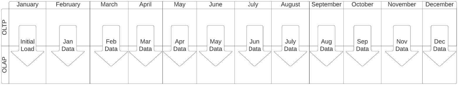
FIGURE 3.23 Delta load example
The frequency with which delta loads happen depends on business requirements. Depending on how fresh the data needs to be, delta loads can happen at any interval. Hourly, daily, and weekly refreshes are typical.
When moving data between systems, you have to balance the speed and complexity of the overall operation. Suppose you operate nationally within the United States and start processing transactions at 7 in the morning and finish by 7 in the evening. The 12 hours between 7 p.m. and 7 a.m. represent the batch window, or time period available, to move data into your data warehouse. The duration of a batch window must be taken into account when designing a delta load strategy.
Data Collection Methods
Augmenting data from your transactional systems with external data is an excellent way to improve the analytical capabilities of your organization. For example, suppose you operate a national motorcycle rental fleet and want to determine if you need to rebalance your fleet across your existing locations. You also want to evaluate whether it is profitable to expand to a new geographic region, as well as predict the best time and place to add motorcycles to your fleet.
Your internal data is a good place to start when analyzing how to grow your business. To improve the accuracy of your analysis, you want to include data about the weather, tourism, and your competitors. This additional data can come from various sources, including federal and state open data portals, other public data sources, and private purveyors of data.
Application Programming Interfaces (APIs)
An application programming interface (API) is a structured method for computer systems to exchange information. APIs provide a consistent interface to calling applications, regardless of the internal database structure. Whoever calls an API has no idea whether a transactional or analytical data store backs it. The internal data structure does not matter as long as the API returns the data you want. APIs can be transactional, returning data as JSON objects. APIs can also facilitate bulk data extraction, returning CSV files.
APIs represent a specific piece of business functionality. Let's return to our motorcycle rental business. Say a repeat customer logs into the website. The web application looks up their profile information, including their name and most frequently visited locations, to personalize their experience. To provide excellent customer service, you want that same information to be available to customer service agents who answer phone calls.
In the top half of Figure 3.24, the SQL to extract customer profile information exists in both the web application and customer service system. This code duplication makes maintenance a challenge—when the SQL needs to change, it has to happen in two places.
The bottom half of Figure 3.24 illustrates the benefit of using an API. Instead of directly embedding SQL in two places, you wrap it in a single GetProfile API. You can easily connect the API to the customer-facing web server and internal-facing customer service system. Suppose you have another application that needs to extract profile information. In that case, all you have to do is connect it to the GetProfile API.
Web Services
Many smartphone applications need a network connection, either cellular or Wi-Fi, to work correctly. The reason is that much of the data these applications need is not on the smartphone itself. Instead, data is found in private and public data sources and is accessible via a web service. A web service is an API you can call via Hypertext Transfer Protocol (HTTP), the language of the World Wide Web.
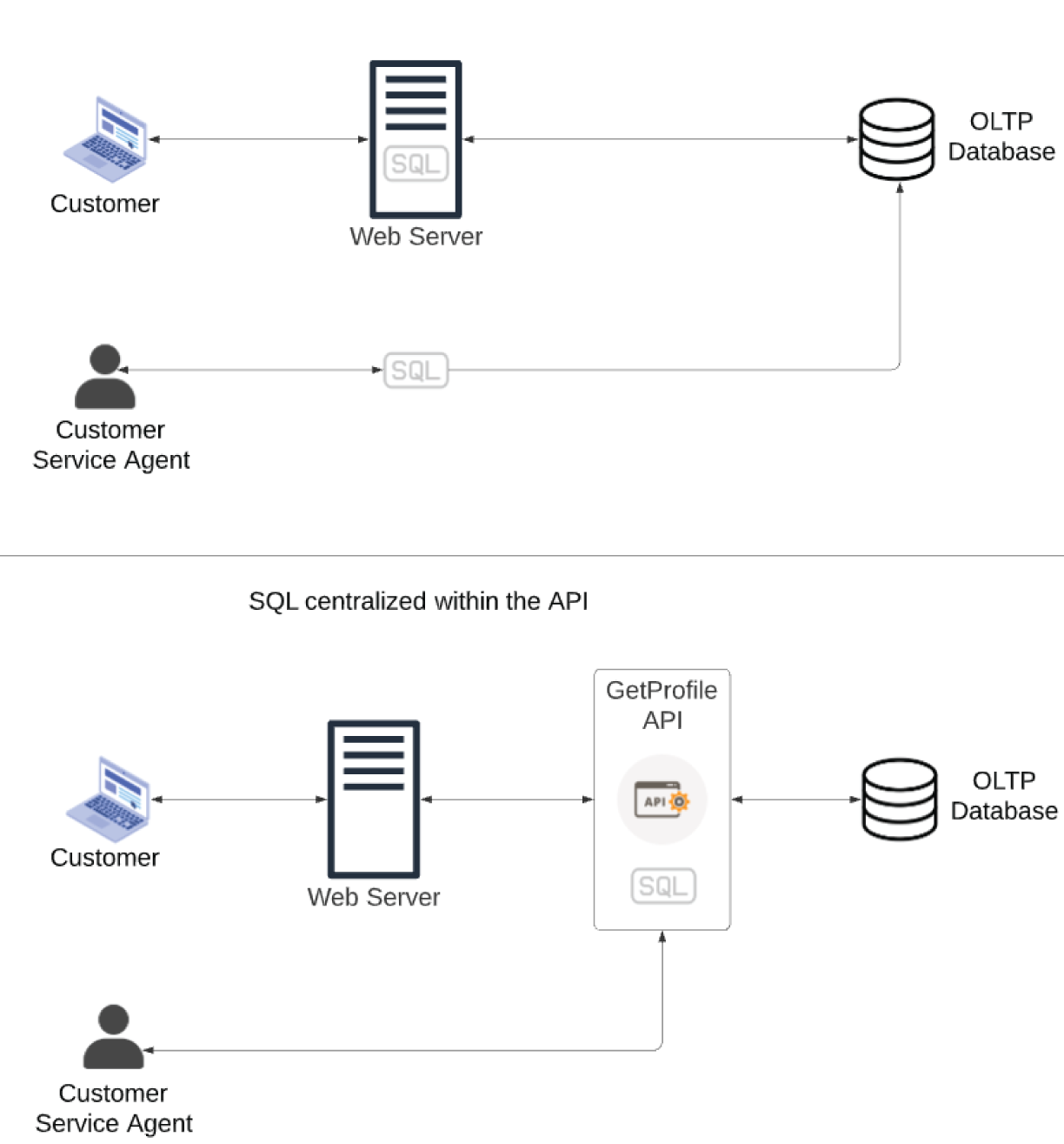
FIGURE 3.24 Internal API example
While a web service is an API, an API does not have to be a web service. Consider the customer service system from Figure 3.24. You might need to install it on each customer service agent's computer, the same way you install Microsoft Excel or PowerPoint, instead of making it a web application. If this is the case, the application accesses the API directly, not as a web service.
Suppose you want to get weather-related data. The National Centers for Environmental Information (NCEI) is a U.S. federal agency within the National Oceanic and Atmospheric Administration (NOAA) office. The NCEI is an authoritative source for weather data. It makes that data available to the public via a web service–enabled API.
Many APIs, like those available from the NCEI, require an API key. If you imagine an API as the door behind which data treasures exist, an API key is what unlocks the door. API providers generate a unique API key for each calling application. Centralized creation and distribution of API keys allow the provider to understand who is using the API and to turn off individual keys' access in the event of abuse.
Open data providers like NCEI make API keys available for free. You register for an API using an email address. After registering, you receive your unique API key in an email. Other data purveyors charge for API access. For example, Google has excellent APIs for static and dynamic map information. In addition to having to register for an API, you incur a nominal charge for each API call. The more you use an API, the more you have to pay. Other API providers take a tiered approach, where you get a limited number of API calls for free, after which you have to pay.
Web Scraping
Some of the data you want may not be available internally as an API or publicly via a web service. However, data may exist on a website. As seen in Chapter 2, data can present itself in an HTML table on a web page. If data exists in a structured format, you can retrieve it programmatically. Programmatic retrieval of data from a website is known as web scraping.
You can use software bots to scrape data from a website. Many modern programming languages, including Python and R, make it easy to create a web scraper. Instead of using an API or a web service, a web scraper reads a web page similar to a browser, such as Chrome, Safari, or Edge. Web scrapers read and parse the HTML to extract the data the web pages contain.
The search results for some websites span multiple web pages. Your web scraper has to account for pagination to ensure that you are not leaving any data behind. The scraper must understand how many result pages exist and then iterate through them to harvest the data.
Human-in-the-Loop
There are times when the data you seek exists only in people's minds. For example, you can extract the most popular and profitable motorcycling destination from your existing internal data. You can get weather information from an API packaged as a web service. You can glean insight into competitive pricing by scraping your competitors' websites. Even with all of these data sources, you may still want insight into how customers feel about the services you provide.
Surveys
One way to collect data directly from your customers is by conducting a survey. The most simplistic surveys consist of one question and indicate customer satisfaction. For example, Figure 3.25 illustrates a survey collection approach in the airline industry. As people board their aircraft, they walk past a small machine with two buttons on it. In response to the question, the people press either the happy face or the unhappy face. Although single-question surveys don't provide any depth as to why people feel positively or negatively, they provide an overall indicator of satisfaction.

FIGURE 3.25 Single question survey
Surveys can be much more complicated than a single question. For example, suppose you want a comprehensive understanding of customer satisfaction. In that case, you design a sophisticated survey that presents people with different questions depending on their answers. Complex survey logic lets you gather additional detail as to why a person has a particular opinion.
You can design surveys to achieve your data collection goals and your audience. You can tailor a survey to collect data on how your employees feel about the effectiveness of their manager, or more broadly, about your organization's approach to pay and benefits. You may want feedback on a customer appreciation event or training session. As long as you know the objective of a survey, you can design one to accomplish your goals.
As you can imagine, survey design is an entire discipline. As you design a survey, you want to keep in mind how you will analyze the data you collect. Numeric data is easy to analyze using a variety of statistical methods. Free-response questions result in unstructured text data, which is more challenging to interpret. You need to clearly understand what is essential to your organization and what decisions you will make using the output to develop and administer an impactful survey.
Observation
Observation is the act of collecting primary source data, from either people or machines. Observational data can be qualitative or quantitative. Collecting qualitative observational data leads to unstructured data challenges.
Imagine observing a person as they perform their work and interact with their colleagues. When you take this approach, it is hard to account for nonverbal communication. You also may struggle to collect data about what people do subconsciously. Returning to our motorcycle rental business, imagine a mechanic going through a post-rental examination. He may augment the post-ride checklist with his experience and intuition. For example, he may decide to change the brake pads and tighten the clutch lever if he perceives the motorcycle was subject to abuse. That may lead him to intuitively look at particular areas of the vehicle for indications of abuse before signing off on the security deposit return.
Asking someone to write down everything they do or the number of times they do something can introduce bias into the data. Developing methods for observation is one way to record what is happening in an environment accurately. Of course, you need to account for the bias of the observer.
Quantitative observations are much easier to collect and interpret. For example, suppose you are trying to establish the defect rate on a production line. You can count the number of vehicles that come off the line, as well as how many fail post-production quality checks.
Sampling
Regardless of the data acquisition approach, you may end up with more data than is practical to manipulate. Imagine you are doing analytics in an Internet-of-Things environment, in which 800 billion events occur daily. Though it is possible, ingesting and storing 800 billion records is a challenging task. Manipulating 800 billion records takes a lot of computing power.
Suppose you want to analyze one day's worth of data. In that case, the 800 billion records represent the total population, or the number of events, available. Since manipulating 800 billion records is unwieldy, you might collect a sample, or subset, of the overall population. Once you have collected sample data, you can use statistical methods to make generalizations about the entire population. For more detail on these methods, see Chapter 5, “Data Analysis and Statistics.”
Working with Data
Determining an appropriate database structure, identifying data sources, and loading a database takes a considerable amount of effort. To turn a database design into an operational database ready to accept data, you use the Data Definition Language (DDL) components of SQL. DDL lets you create, modify, and delete tables and other associated database objects.
With all of that work complete, the foundation is in place to derive impactful insights. To generate insights, a productive analyst must be comfortable using the Data Manipulation Language (DML) capabilities of SQL to insert, modify, and retrieve information from databases. While DDL manages the structure of a database, DML manages the data in the database.
The DML components of SQL change very slowly. As long as relational databases exist, you will need to understand SQL to work with them. It is worth learning SQL, as the foundational knowledge of DML operations will serve you well.
Data Manipulation
When manipulating data, one of four possible actions occurs:
- Create new data.
- Read existing data.
- Update existing data.
- Delete existing data.
The acronym CRUD (Create, Read, Update, Delete) is a handy way to remember these four operations.
SQL uses verbs to identify the type of activity a specific statement performs. For each CRUD activity, there is a corresponding DML verb, as Table 3.8 illustrates. These verbs are known as keywords, or words that are part of the SQL language itself.
TABLE 3.8 Data manipulation in SQL
| Operation | SQL Keyword | Description |
|---|---|---|
| Create | INSERT | Creates new data in an existing table |
| Read | SELECT | Retrieves data from an existing table |
| Update | UPDATE | Changes existing data in an existing table |
| Delete | DELETE | Removes existing data from an existing table |
Reading and manipulating data is commonplace on the path to creating insights. To that end, we will focus on options that affect reading data. Before jumping in, it is helpful to understand the syntax of a query.

FIGURE 3.27 SQL SELECT statement
Figure 3.27 illustrates the basic structure of a SQL query that reads from a database. SELECT, FROM, and WHERE are all reserved words that have specific meaning in SQL.
The SELECT clause identifies the columns from the table(s) that are retrieved. If you want to list the name and animal type from Table 3.1, the SELECT portion of the query will look like this:
SELECT Animal_Name, Breed_Name
The FROM clause in a query identifies the source of data, which is frequently a database table. Both the SELECT and FROM clauses are required for a SQL statement to return data, as follows:
SELECT Animal_Name, Breed_NameFROM Animal
As the queries in Figure 3.21 illustrate, it is possible to specify more than one location for data by joining tables together.
Filtering
Examining a large table in its entirety provides insight into the overall population. To answer questions that an organization's leadership has typically requires a subset of the overall data. Filtering is a way to reduce the data down to only the rows that you need.
To filter data, you add a WHERE clause to a query. Note that the column you are filtering on does not have to appear in the SELECT clause. To retrieve the name and breed for only the dogs from Table 3.1, you modify the query as follows:
SELECT Animal_Name, Breed_NameFROM AnimalWHERE Animal_Type = 'Dog'
Filtering and Logical Operators
A query can have multiple filtering conditions. You need to use a logical operator to account for complex filtering needs. For example, suppose you need to retrieve the name and breed for dogs weighing more than 60 pounds. In that case, you can enhance the query using the AND logical operator, as follows:
SELECT Animal_Name, Breed_NameFROM AnimalWHERE Animal_Type = 'Dog'AND Weight> 60
The AND operator evaluates the Animal_Type and Weight filters together, only returning records that match both criteria. OR is another frequently used logical operator. For example, suppose you want to see the name and breed for all dogs and any animals that weigh more than 10 pounds regardless of the animal type. The following query delivers the answer to that question:
SELECT Animal_Name, Breed_NameFROM AnimalWHERE Animal_Type = 'Dog'OR Weight> 10
Complex queries frequently use multiple logical operators at the same time. It is good to use parentheses around filter conditions to help make queries easy for people to read and understand.
Data warehouses often contain millions, billions, or even trillions of individual data records. Filtering data is essential to making effective use of these massive data stores.
Sorting
When querying a database, you frequently specify the order in which you want your results to return. The ORDER BY clause is the component of a SQL query that makes sorting possible. Similar to how the WHERE clause performs, you do not have to specify the columns you are using to sort the data in the SELECT clause.
For example, suppose you want to retrieve the animal and breed for dogs over 60 pounds, with the oldest dog listed first. The following query delivers the answer:
SELECT Animal_Name, Breed_NameFROM AnimalWHERE Animal_Type = 'Dog'AND Weight> 60ORDER BY Date_of_Birth ASC
If you want to return the youngest dog first, you change the ORDER BY clause as follows:
SELECT Animal_Name, Breed_NameFROM AnimalWHERE Animal_Type = 'Dog'AND Weight> 60ORDER BY Date_of_Birth DESC
The ASC keyword at the end of the ORDER BY clause sorts in ascending order whereas using DESC with ORDER BY sorts in descending order. If you are sorting on multiple columns, you can use both ascending and descending as appropriate. Both the ASC and DESC keywords work across various data types, including date, alphanumeric, and numeric.
Date Functions
As seen in Table 3.5 and Table 3.6, date columns are frequently found in OLAP environments. Date columns also appear in transactional systems. Storing date information about an event facilitates analysis across time. For example, you may be interested in first-quarter sales performance or outstanding receivables on a rolling 60-day basis. Fortunately, there is an abundance of functions that make working with dates easy.
The most important thing to note is that you have to understand the database platform you are using and how that platform handles dates and times. Since each platform provider uses different data types for handling this information, you need to familiarize yourself with the functions available from your provider of choice.
Logical Functions
Logical functions can make data substitutions when retrieving data. Remember that a SELECT statement only retrieves data. The data in the underlying tables do not change when a SELECT runs. Consider Table 3.9, which enhances Table 3.1 by adding a Sex column. Looking at the values for Sex, we see that this column contains code values. To understand the description for each code value in a sound relational model, the Sex column from Table 3.9 is a foreign key pointing to the Sex column in Table 3.10.
TABLE 3.9 Augmented animal data
| Animal_ID | Animal_Name | Animal_Type | Breed_Name | Sex | Date_of_Birth | Height (inches) | Weight (pounds) |
|---|---|---|---|---|---|---|---|
| 1 | Jack | Dog | Corgi | M | 3/2/2018 | 10 | 26.3 |
| 2 | Viking | Dog | Husky | M | 5/8/2017 | 24 | 58 |
| 3 | Hazel | Dog | Labradoodle | F | 7/3/2016 | 23 | 61 |
| 4 | Schooner | Dog | Labrador Retriever | M | 8/14/2019 | 24.3 | 73.4 |
| 5 | Skippy | Dog | Weimaraner | F | 10/3/2018 | 26.3 | 63.5 |
| 6 | Alexander | Cat | American Shorthair | M | 10/4/2017 | 9.3 | 10.4 |
TABLE 3.10 Sex Lookup Table
| Sex | Sex_Description |
|---|---|
| M | Male |
| F | Female |
Suppose you want to retrieve the name and sex description for each animal, as Table 3.11 illustrates. One way to accomplish this is by joining the two tables together, retrieving the Animal_Name from Table 3.9 and Sex_Description from Table 3.10.
TABLE 3.11 Desired Query Results
| Animal_Name | Sex |
|---|---|
| Jack | Male |
| Viking | Male |
| Hazel | Female |
| Schooner | Male |
| Skippy | Female |
| Alexander | Male |
When writing SQL, there are frequently many ways to write a query and create the same results. Another way to generate the output in Table 3.10 is by using the IFF logical function. The IFF function has the following syntax:
IFF(boolean_expression, true_value, false_value)
As you can see from the syntax, the IFF function expects the following three parameters:
- Boolean Expression: The expression must return either TRUE or FALSE.
- True Value: If the Boolean expression returns TRUE, the
IFFfunction will return this value. - False Value: If the Boolean expression returns FALSE, the
IFFfunction will return this value.
The following query, using the IFF function, generates the results in Table 3.11:
SELECT Animal_Name, IFF(Sex = 'M', 'Male', 'Female')FROM Animal
Note that with the IFF approach, the values for Male and Female come from the function parameters, not from the source table (Table 3.9). Suppose the description in the underlying table gets modified. In that case, the results of the IFF query will not reflect the modified data.
Table 3.12 shows the results of the following query, which also uses the IFF function:
SELECT Animal_Name, IFF(Sex = 'M', 'Boy', 'Girl')FROM Animal
TABLE 3.12 Modified IFF query results
| Animal_Name | Sex |
|---|---|
| Jack | Boy |
| Viking | Boy |
| Hazel | Girl |
| Schooner | Boy |
| Skippy | Girl |
| Alexander | Boy |
IFF is just one example of a logical function. When using logical functions, you need to balance their convenience with the knowledge that you are replacing data from the database with the function's coded values. The ability to do this type of substitution is a real asset when dividing data into categories.
Aggregate Functions
Summarized data helps answer questions that executives have, and aggregate functions are an easy way to summarize data. Aggregate functions summarize a query's data and return a single value. While each database platform supports different aggregation functions, Table 3.13 describes functions that are common across platforms. Be sure to familiarize yourself with the functions available in your platform of choice.
TABLE 3.13 Common SQL aggregate functions
| Function | Purpose |
|---|---|
COUNT | Returns the total number of rows of a query. |
MIN | Returns the minimum value from the results of a query. Note that this works on both alphanumeric and numeric data types. |
MAX | Returns the maximum value from the results of a query. Note that this works on both alphanumeric and numeric data types. |
AVG | Returns the mathematic average of the results of a query. |
SUM | Returns the sum of the results of a query. |
STDDEV | Returns the sample standard deviation of the results of a query. |
You can also use aggregate functions to filter data. For example, you may want a query that shows all employees who make less than the average corporate salary. Aggregate functions also operate across subsets of data. For instance, you can calculate total sales by month with a single query.
System Functions
Each database platform offers functions that expose data about the database itself. One of the most frequently used system functions returns the current date. The current date is a component of transactional records and enables time-based analysis in the future. The current date is also necessary for a system that uses an effective date approach.
System functions also return data about the database environment. For example, whenever a person or automated process uses data from a database, they need to establish a database session. A database session begins when a person/program connects to a database. The session lasts until the person/program disconnects. For example, a poorly written query can consume most of the resources available to the database. When that happens, a database administrator can identify and terminate the problematic session.
Query Optimization
Writing a SQL query is straightforward. Writing a SQL query that efficiently does what you intend can be more difficult. There are several factors to consider when creating well-performing SQL.
Parametrization
Whenever a SQL query executes, the database has to parse the query. Parsing translates the human-readable SQL into code the database understands. Parsing takes time and impacts how long it takes for a query to return data. Effective use of parameterization reduces the number of times the database has to parse individual queries.
Suppose you operate a website and want to personalize it for your customers. Login details serve as parameters to the query to retrieve your information for display. After logging in, a customer sees a welcome message identifying them by name.
Figure 3.28 provides an example of the web server creating a hard-coded query. Examining the WHERE filter in the query, we see that it matches the string “Gerald.” When Gerald logs in, the database parses the query, executes it, and returns Gerald's information.
In this situation, when Gina logs in, the WHERE filter looks specifically for “Gina.” Since “Gerald” is different from “Gina,” the database treats this as a new query and parses it. The time it takes to parse becomes problematic at scale. Imagine 1,000 people all logging in at the same time. The database sees each of these queries as unique and ends up parsing 1,000 times.

FIGURE 3.28 Hard-coded SQL query
Figure 3.29 illustrates how to address this potential performance problem using parameterization. Instead of looking specifically for an exact string match for every customer, the query uses a variable called &customer_name. The code in the web server populates the variable with the appropriate customer name. To the database, this appears as a single query. While the value of &customer_name changes for every customer, the database parses it only once.
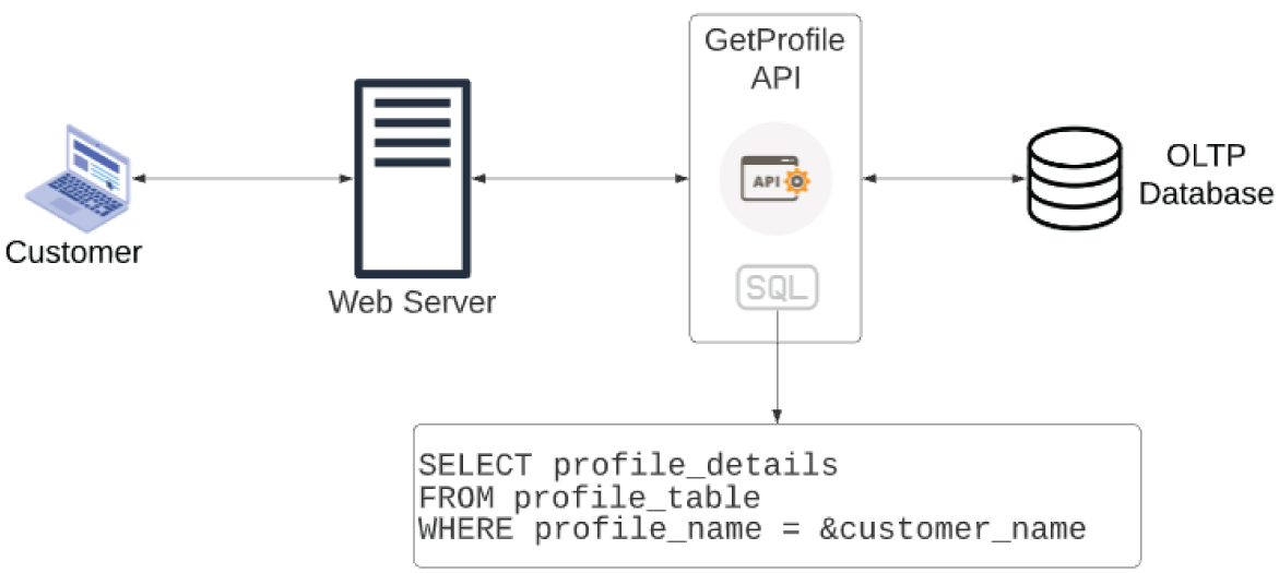
FIGURE 3.29 Parameterized SQL query
Indexing
When retrieving data from a table, the database has to scan each row until it finds the ones that match the filters in the WHERE clause. The process of looking at each row is called a full table scan. A full table scan is like flipping through every page in a book to find a specific piece of data. For small tables, full table scans happen quickly. As data volumes increase, scanning the entire table takes a long time and is not efficient. To speed up query performance, you need a database index.
A database index works like the index in the back of a book. Instead of looking at each page in a book to find what you are looking for, you can find a specific page number in the index and then go to that page.
A database index can point to a single column or multiple columns. When running queries on large tables, it is ideal if all of the columns you are retrieving exist in the index. If that is not feasible, you at least want the first column in your SELECT statement to be covered by an index.
If a query is running slowly, look at the indexes on the underlying tables. If you think a new index would help improve query performance, discuss it with a database administrator. The administrator will look at other factors that impact performance and will have the permissions to create an index if necessary.
While indexing improves query speed, it slows down create, update, and delete activity. An indexing strategy needs to match the type of system the database supports, be it transactional or reporting.
Data Subsets and Temporary Tables
When dealing with large data volumes, you may want to work with a subset of records. For example, suppose an organization has 1,000,000 customers. Each of those customers places 200 orders per year, and there are 10 years of data in the data warehouse. In this situation, the Order table in the data warehouse would have 2 billion rows. If you want to explore trends for a specific customer's order history, it would not be efficient to query the main Order table.
It is possible to create a temporary table to make the data more manageable. Temporary tables can store the results of a query and are disposable. Temporary tables automatically get removed when the active session ends. Using temporary tables is an effective method of creating subsets for ad hoc analysis.
For example, you can establish a database session, create a temporary table with the order history for a single customer, run queries against that temporary table, and disconnect from the database. When the session disconnects, the database automatically purges any temporary tables created during the session.
Execution Plan
An execution plan shows the details of how a database runs a specific query. Execution plans are extremely helpful in troubleshooting query performance issues. They provide additional information about how a query is spending its time.
For example, an execution plan can tell you if a slow-running query uses a full table scan instead of an index scan. In this case, it could be that the query is poorly written and not using the existing indexes. It also could be that a column needs a new index.
Looking at execution plans is an integral part of developing efficient queries. It is worth understanding the nuances of how to interpret execution plans for the database platform you use. If you need help understanding an execution plan, get in touch with your local database administrator.
Summary
Databases are technology platforms for processing and storing data. There are two primary types of databases: relational and non-relational. Relational databases are ideal when you have tabular data, while there are numerous non-relational offerings when you need more flexibility than the structure a relational database imposes.
Using a relational database as a technology platform, you can build transactional or analytical databases to address the business need. Transactional (OLTP) and analytical (OLAP) databases require different schema design approaches. Since a transactional database needs to balance reading and writing data, it follows a highly normalized schema design.
On the other hand, analytical databases prioritize reading data and follow a denormalized approach. The star and snowflake schema designs are two approaches to structuring data for analysis. Both methods implement dimensional modeling, which organizes quantitative data into facts and qualitative data into dimensions.
There are multiple ways to acquire data for analysis. For example, most data warehouses source data from transactional systems. To copy data from a transactional system, you can use an ETL or ELT approach. ETL leverages technology external to a relational database to transform data, while ELT uses the power of a relational database to do the transformation. Depending on the rate of change and data volume, you can take a complete refresh or delta load approach.
You can also acquire data from external sources. APIs are integration components that encapsulate business logic and programmatically expose data. It is common to interact with APIs to source data for both transactional and analytical purposes. You may also find yourself needing to scrape data from a website or pull data from a public database.
There are times when you need primary source data that you can't obtain programmatically. In that case, you may end up conducting a survey or observing people and processes.
Once you have data in a relational database, you need to be comfortable manipulating it. Structured Query Language (SQL) is the standard for relational data manipulation. With SQL queries, you can filter, sort, compare, and aggregate data.
There are times when you will be working with large volumes of data that impact performance. There are several approaches you can take to mitigate performance issues. When writing frequently executed queries, make sure you use parametrization to reduce the database's parsing load. Reducing the number of records you're working with is another viable approach, which you can achieve by subsetting the data and using temporary tables. If you have queries taking more time than you expect, work with a database administrator to review the query's execution plan and ensure you have the appropriate indexing strategy.
Exam Essentials
Describe the characteristics of OLTP and OLAP systems. The two main categories of relational databases are transactional (OLTP) and analytical (OLAP). Transactional systems use highly normalized schema design, which allows for database reads and writes to perform well. Analytical systems are denormalized and commonly have a star or snowflake schema. Remember that a star design simplifies queries by having a main fact table surrounded by dimensions. A snowflake design is more normalized than a star. While this approach reduces storage requirements, the queries are more complex than in a star schema.
Describe approaches for handling dimensionality. It is crucial to keep track of how data changes over time to perform historical analysis. Although an effective date approach is valid, the SQL queries to retrieve a value at a specific point in time are complex. A table design that adds start date and end date columns allows for more straightforward queries. Enhancing the design with a current flag column makes analytical queries even easier to write.
Understand integration and how to populate a data warehouse. The more data an organization has, the more impactful the analysis it can conduct. The extract, transform, and load (ETL) process copies data from transactional to analytical databases. Suppose an organization wants to use the power of a relational database to reformat the data for analytical purposes. In that case, the order changes to extract, load, and transform. Regardless of the approach, remember that a delta load migrates only changed data.
Differentiate between data collection methods. Data can come from a variety of sources. An organization may scrape websites or use publicly available databases to augment its data. While web scraping may be the only way to retrieve data, it is better if a published application programming interface exists. An API is more reliable since its structure makes for a consistent interface. If you want to capture the voice of the customer, a survey is a sound approach. Collecting data through observation is a great way to validate business processes and collect quantitative data.
Describe how to manipulate data and optimize queries. Analytical databases store massive amounts of data. Manipulating the entire dataset for analysis is frequently infeasible. To efficiently analyze data, understand that SQL has the power to filter, sort, and aggregate data. When focusing on a particular subject, creating a subset is an ideal approach. Although it is possible to create permanent tables to house subsets, using a temporary table as part of a query is viable for ad hoc analysis. When an analytical query performs poorly, use its execution plan to understand the root cause. It is wise to work with a database administrator to understand the execution plan and ensure that indexes exist where they are needed.
Review Questions
- Claire operates a travel agency and wants to automatically recommend accommodation, rental car, and entertainment packages based on her customers' interests. What type of database should Claire select?
- Relational
- Graph
- Key-value
- Column-family
- Evan needs to retrieve information from two separate tables to create a month-end credit card summary. What should he use to join the tables together?
- Primary key
- Foreign key
- Synthetic primary key
- Referential integrity
- Taylor wants to investigate how manufacturing, marketing, and sales expenditures impact overall profitability for her company. Which of the following systems is most appropriate? Choose the best answer.
- OLTP
- OLAP
- Data warehouse
- Data mart
- J. R. needs to move data into his data warehouse. One of his primary concerns is how fast data can get into the warehouse. As he thinks about approaches for transferring data, which of the following is the best option?
- Initial load
- Delta load
- ETL
- ELT
- Riley is designing a data warehouse and wants to make writing queries that track customer satisfaction over time as simple as possible. What could she add to her table design to accomplish her goal? Choose the best answer.
- Current flag
- Start date
- Middle date
- End date
- Richard is designing a data warehouse and wants to minimize query complexity. What design pattern should he follow?
- Avalanche
- Star
- Snowflake
- Quasar
- Razia is working on understanding population trends by county across the United States. Considering the rate of change, which of the following best describes county name?
- Static dimension
- Slowly changing dimension
- Rapidly changing dimension
- Fluid dimension
- Zaiden is debating between a snowflake and a star schema design for a data warehouse. Which of the following is not a factor in his selection?
- Storage space
- Query complexity
- Number of records in the fact table
- Degree of normalization
- Madeline wants to collect data about how her competitor prices products. She can see this information after logging in to her competitor's website. After some initial struggles, Madeline creates a web scraper to harvest the data she needs. What does she need to do next? Choose the best answer.
- Check the terms of service.
- Load the data into an OLTP database.
- Load the data into an OLAP database.
- Figure out how to parse JSON.
- Maurice manages an organization of software developers with deep expertise in Python. He wants to make use of this expertise to move data between transactional systems and the data warehouse. In what phase are Python skills most relevant?
- Extract
- Transform
- Load
- Purge
- Ellen is collecting data about a proprietary manufacturing process and wants to control for any bias that workers may have. What type of data collection approach is most appropriate?
- Survey
- Sample
- Public database
- Observation
- George wants to integrate data from his city's open data portal. Reading the website, he sees that he can download the data he wants as a CSV file. After manually downloading the file, he writes the code to transform the data and load it into his database. Presuming the data changes once a month, what can George do to ensure he has the most up-to-date data from the city? Choose the best answer.
- Manually check the city's website every day.
- Contact the city and encourage the development of an API.
- Automate the process that downloads, transforms, and uploads the CSV file.
- Nothing, George has already successfully loaded the data.
- Martha is designing a nightly ETL process to copy data from an order processing system into a data warehouse. What should she do to replicate the data she needs efficiently without losing historical data? Choose the best answer.
- Complete purge and load
- Delta load
- ELT
- Use an ETL product
- Bob manages a production line and is worried that defects are not being accurately reported. What is the best way for him to obtain the true number of defects?
- Survey the production staff.
- Test a sample of finished goods.
- Observe the final quality check process.
- Use historical data to establish a trend.
- Barb wants to understand which product costs the least. What aggregate function can she use in her SQL query to get this answer?
COUNTMAXMINAVG
- Elena is an analyst at a multinational corporation. She wants to focus her analysis on transactions that took place in Italy. What is the first thing she should do to make efficient use of resources?
- Filter out transactions for all countries except Italy.
- Filter out transactions for Italy.
- Aggregate transactions across the European Union.
- Subset the data to a specific Italian province.
- Jeff is an analyst at a company that operates in the United States. He wants to understand profitability trends by region, state, and county. What should he do next? Choose the best answer.
- Aggregate data at the county level.
- Aggregate data by region, state, and county.
- Use effective date logic to determine current profitability.
- Make sure there is an index on the county column.
- Gretchen is trying to create a list of purchases in chronological order. What clause does she need to add to her SQL query?
SELECTFROMWHEREORDER BY
- Brandon is trying to understand why the personalization features of his website performs poorly under heavy load. Looking at the query that retrieves customer profile information, he sees that the web application is hard-coding the customer's identifying number into each query, then using the Customer_ID column to retrieve profile data. Looking at the execution plan, Brandon sees that the query is performing optimally. What does he need to do to resolve the performance issue? Choose the best answer.
- Check to ensure there is an index to the Customer_ID column.
- Review the execution plan for the query with a DBA.
- Remove the personalization features due to the performance problems.
- Change the application code to use query parameters instead of hard-coding.
- Julie wants to retrieve the total number of rows in a table. Which aggregation function should she use in her SQL query?
STDDEVCOUNTSUMMAX