
Chapter 9
Prospective Mortality Tables and Portfolio Experience
Julien Tomas
Université de Lyon 1
Lyon, France
Frédéric Planchet
Université de Lyon 1 - Prim'Act
Lyon, France
9.1 Introduction and Motivation
In this chapter1, we will describe an operational framework for constructing and validating prospective mortality tables specific to an insurer. The material is based on studies2 carried out by the Institut des Actuaries. This research has been conducted with the aim of providing to French insurance companies methodologies to take into account their own mortality experience for the computation of their best estimate reserves.
We will present several methodologies and the process of validation allowing an organism to adjust a mortality reference to get closer to a best estimate adjustment of its mortality and longevity risks. The techniques proposed are based only on the two following elements:
- ● A reference of mortality
- ● Data, line by line originating from a portfolio provided by the insurer
Various methods of increasing complexity will be presented. They allow the organism some latitude of choice while preserving simplicity of implementation for the basic methodology. In addition, they provide a simple adjustment without the intervention of an expert.
The simplest approach is the application of a single factor of reduction / increase to the probabilities of death of the reference. In practice, this coefficient is the Standardized Mortality Ratio (SMR) of the population considered. The second method is a semiparametric Brass-type relational model. This model implies that the differences between the observed mortality, and the reference can be represented linearly with two parameters. For the third method, we will consider a Poisson generalized linear model including the baseline mortality of the reference as a covariate and allowing interactions with age and calendar year. The fourth method includes, in a first step, a nonparametric smoothing of the periodic table and, in a second step, the application of the rates of mortality improvement derived from the reference.
The validation will be assessed on three levels. The first level concerns the proximity between the observations and the model. It is assessed by the likelihood ratio test, the SMR test, and the Wilcoxon Matched-Pairs Signed-Ranks test. As a complement, the validation of the fit involves graphical diagnostics such as the analysis of the response, Pearson and deviance residuals, as well as the comparison between the predicted and observed mortality by attained age and calendar year. The second level involves the regularity of the fit. It is assessed by the runs test and signs test. Finally, the third level covers the plausibility and consistency of the mortality trends. It is evaluated by single indices summarizing the lifetime probability distribution for different cohorts at several ages. Moreover, it involves graphical diagnostics assessing the consistency of the observed and forecasted life expectancy. Additionally, if we have at our disposal the male and female mortality, we can compare the improvement and judge the plausibility of the common evolution of the mortality of the two genders. We ask the question where are the data originating from and based on this knowledge, what mixture of biological factors, medical advances and environmental changes would have to happen to cause this particular set of forecasts?
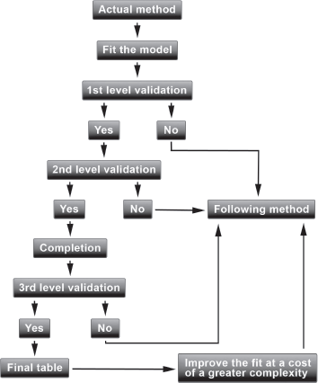
The methods articulate around an iterative procedure allowing one to compare them and to choose parsimoniously the most satisfying one. We will present an operational framework based on the software R and on the package ELT available on CRAN. Briefly, the procedure is as follows. We will start with the first method; if the criteria corresponding to the first level of validation are not satisfied, we then switch to the second method as it is useless to continue the validation with the first method. If the criteria corresponding to the first level are satisfied, we continue the validation with the criteria of the second level. We can also turn to the following method to improve the fit at a cost of somewhat greater complexity without degrading the results of the criteria of the first level. The process of validation is summarized in Figure 9.1.
9.2 Notation, Data, and Assumption
We analyze the mortality as a function of both the attained age x and the calendar year t. The number of individuals at attained age x during calendar year t is denoted by Lx,t, and Dx,t represents the number of deaths recorded from an exposure-to-risk Ex,t that measures the time during which individuals are exposed to the risk of dying. It is the total time lived by these individuals during the period of observation. The probability of death at attained age x for the calendar year t is denoted by qx(t) and computed according to the Hoem estimator, qx(t)=Dx,tEx,t We suppose that we have data line by line, originating from a portfolio, with a comma-separated variable in a csv file. The variables
- Gender with modalities Male and/or Female,
- DateOfBirth, DateIn, and DateOut,
- Status with modalities other and deceased,
should imperatively appear as displayed below:
Id Gender DateOfBirth DateIn DateOut Status
100001 Female 1973/10/10 1995/12/01 2003/12/01 other
100002 Male 1901/05/12 1996/01/01 2001/04/21 deceased
100003 Female 1970/07/10 1995/11/01 2000/02/01 other
100004 Male 1916/07/07 1996/01/01 2002/01/28 deceased
100005 Female 1950/10/31 1995/11/01 2003/11/01 other
100006 Male 1918/04/06 1996/01/01 2002/06/01 deceased
The data in input should ideally be validated by the organism and it is supposed that they can be used without re-treatment.
Table 9.1 presents the observed characteristics of the male and female population of the data MyPortfolio used for our application. These are real data that, for confidentiality reasons, are composed by a mix of portfolios and, in consequence, can present atypical behaviors. We refer to Tomas & Planchet (2013) for additional illustrations of the methodologies proposed.
Observed characteristics of the male and female population of the portfolio.
Mean Age In |
Mean Age Out |
Average Exposition |
Mean Age at Death |
Period of Observation |
||
Beginning |
End |
|||||
Male pop. |
42.27 |
49.69 |
7.42 |
70.31 |
1996/01/01 |
2007/12/31 |
Female pop. |
45.09 |
52.91 |
7.81 |
81.01 |
1996/01/01 |
2007/12/31 |
To each of the observations i, we associate the dummy variable δi indicating if the individual i dies or not,
δi={1 if individual i dies,0 otherwise,
for i = 1,..., Lx,t We define the time lived by individual i before (x + 1) th birthday by τi .We assume that we have at our disposal i.i.d. observations (δi,τi) for each of the Lx,t individuals. Then,
∑Lx,ti=1τi=Ex,t et ∑Lx,ti=1δi=Dx,t.
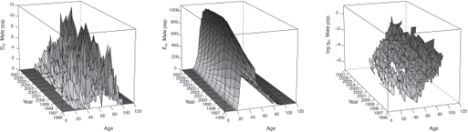
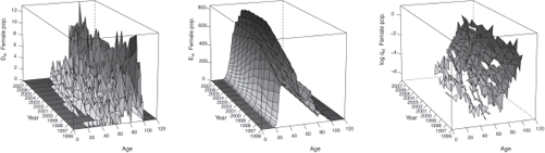
Figures 9.2 and 9.3 display the observed statistics of the male and female population respectively. We refer to Section 10.2 for an example of R codes used to produce such statistics.
In this chapter, we will use the national demographic projections for the French population over the period 2007-2060, provided by the French National Office for Statistics,
INSEE, Blanpain & Chardon (2010) as a reference to adjust the mortality experience of our portfolio. These projections are based on assumptions concerning fertility, mortality, and migrations and we chose the baseline scenario for our application.
9.3 The Methods
In the following, we present the methodological aspects of the four methods considered, as well as the core of the functions contained in the package ELT.
9.3.1 Method 1: Approach Involving One Parameter with the SMR
The approach involving one parameter is the simplest methodology considered. It consists of applying a single factor of reduction / increase to the probability of death of the reference, denoted qrefx(t) . In practice, this coefficient is the Standardized Mortality Ratio (SMR) of the population considered, see Liddell (1984). Then we obtain the probabilities of death of the organism, denoted ˜qx(t), for x∈ [x_,ˉx] et t ∈[t_,ˉt] by
˜qx(t)=SMR × qrefx(t) with SMR = ∑(x*,t*)Dx,t∑(x*,t*)Ex,tqrefx(t),
where x* and t* correspond to the age range and to the period of observation in common with the reference of mortality, respectively. The method is implemented in R as follows:
> FctMethodl = function(d, e, qref, x1, x2, t1, t2){
+ SMR <- sum(d[x1 - min(as.numeric(rownames(d))) + 1,]/ sum(e[x1 -
min(as.numeric(rownames(l))) + 1,] * log(1 - qref[x1 - min(x2) + 1, as.character(t1)])
+ SMR <- mean(SMRxt[SMRxt != 0 & is.na(SMRxt) == F & SMRxt != Inf])
+ QxtFitted <- SMR * qref[, as.character(min(t1) : max(t2))]
+ colnames(QxtFitted) <- min(t1) : max(t2); rownames(QxtFitted) <- x2
+ return(list(SMR = SMR, QxtFitted = QxtFitted, NameMethod = "Method1"))
+ }
In consequence, we adjust the mortality of the organism only with one parameter, the SMR. It represents the observed deviation between the deaths recorded by the organism and the ones predicted by the reference.
The choice of x* is of great importance because the table constructed is only valid on the age range considered and its choice may be complicated. For the male population, after setting the age range, we obtain,
> AgeRange <- 30 : 90
> MIMale <- FctMethod1(MyData$Male$Dxt, MyData$Male$Ext, MyData$Male$QxtRef, AgeRange, MyData$Male$AgeRef, MyData$Male$YearCom, MyData$Male$YearRef)
> print(paste("QxtFittedMale = ",M1Male$SMR," * QxtRefMale"))
[1] "QxtFittedMale = 0.614721542286672 * QxtRefMale"
9.3.2 Method 2: Approach Involving Two Parameters with a Semiparametric Relational Model
The second approach is a semiparametric Brass-type relational model. The fit is performed using the logistic function,
˜qx(t), for x∈ [x_,ˉx] et t ∈[t_,ˉt]
where x*and t* correspond to the age range and to the period of observation in common with the reference, respectively, and qrefx∗(t∗) is the reference of mortality.
This model implies that the differences between the observed mortality and the reference can be represented linearly with two parameters. The parameter a is an indicator of mortality affecting all ages identically while the parameter fi modifies this effect with age. The estimation is done by minimizing a weighted distance between the estimated and observed mortality,
∑|Ex*,t*×(ˆqx*(t*)−ˆqx*(t*))| .
This model has the advantage of integrated estimation and forecasting, as the parameters α and β are constant. We refer to Section 10.4.2 and Planchet & Théerond (2011, Chapter 7) for more details.
We obtain the probabilities of death of the organism ˜qx(t),forx∈[x_,ˉx]et t∈[t_,ˉt] by
˜qx(t)=exp(ˆα + ˆβ logit qrefx(t))1+exp(ˆα+ˆβ logit qrefx(t))
The semiparametric relational model is defined in R with the following functions:
> FctLogit = function(q) {log(q / (1 - q))}
> FctMethod2 = function(d, e, qref, x1, x2, t1, t2){
+ Qxt <- (d[x1 - min(as.numeric(rownames(d))) + 1,] /
e[x1 - min(as.numeric(rownames(l))) +1,])
+ LogitQxt <- FctLogit(Qxt)
+ LogitQxt[LogitQxt == -Inf] <- 0
+ LogitQxtRef <- FctLogit(qref[x1 - min(x2) + 1, as.character(t1)])
+ LogitQxtRef[LogitQxtRef == -Inf] <- 0
+ Distance = function(p){
+ LogitQxtFit <- (p[1] + p[2] * LogitQxtRef)
+ QxtFit <- exp(LogitQxtFit) / (1 + exp(LogitQxtFit))
+ sum(abs(e[x1 - min(as.numeric(rownames(e))) + 1,] * (Qxt - QxtFit)))
+ }
+ ModPar <- constrOptim(c(0, 1), Distance, ui = c(0, 1), ci = 0,
control = list(maxit = 10"3), method = "Nelder-Mead")$par
+ LogitQxtRef <- FctLogit(qref[, as.character(min(t1) : max(t2))])
+ QxtFitted <- as.matrix(exp(ModPar[1] + ModPar[2] * LogitQxtRef) /
(1 + exp(ModPar[1] + ModPar[2] * LogitQxtRef)))
+ colnames(QxtFitted) <- as.character(min(t1) : max(t2))
+ rownames(QxtFitted) <- x2
+ return(list(ModPar = ModPar, QxtFitted = QxtFitted,
NameMethod = "Method2"))
+ }
After setting the age range, we obtain for the male population:
> AgeRange <- 30 : 90
> M2Male <- FctMethod2(MyData$Male$Dxt, MyData$Male$Ext, MyData$Male$QxtRef,
AgeRange, MyData$Male$AgeRef, MyData$Male$YearCom, MyData$Male$YearRef)
> print(paste("logit (QxtFittedMale) = ",M2Male$ModPar[1],"+",M2Male$ModPar[2],"
* logit (QxtRefMale)"))
[1] "logit (QxtFittedMale) = 0.247405963276836 + 1.18826425350273 *
logit (QxtRefMale)"
9.3.3 Method 3: Poisson GLM Including Interactions with Age and Calendar Year
The third approach is a Poisson Generalized Linear Model (GLM) including the baseline mortality of the reference as a covariate and allowing interactions with age and calendar year.
With the notation of Section 9.2 and under the assumption of a piecewise constant force of mortality, the likelihood becomes
L(qx(t))=exp(−Ex,tqx(t))(qx(t))Dx,t.
The associated log-likelihood is
ℓ(qx(t))=logL(qx(t))=−Ex,tqx(t) + Dx,tlogqx(t).
Maximizing the log-likelihood ℓ(qx(t)) gives ˆqx(t)=Dx,t/Ex,tlogqx(t) which coincides with the central death rates ˆmx(t).
It is then apparent that the likelihood ℓ(qx(t)) is proportional to the Poisson likelihood based on
Dx,t∼p(Ex,tqx(t))(9.1)
Thus, it is equivalent to work on the basis of the true likelihood or on the basis of the Poisson likelihood, as recalled in Delwarde, A. & Denuit, M. (2005). In consequence, under the assumption of constant forces of mortality between non-integer values of x and t, we consider (9.1) to take advantage of the GLMs framework.
We suppose that the number of deaths of the organism at attained age x* and calendar year t* is determined by
Dx*,t*∼P(Ex*,t* μx*(t*)),
with μx*(t*)=β0+β1logqrefx*(t*)+β2x*+β3t*+β4x*t*,
where x*and t* correspond to the age range and to the period of observation in common with the reference, respectively, and μrefx*(t*) are the baseline forces of mortality.
If we do not allow for interactions, we will observe parallel shifts of the mortality according to the baseline mortality for each dimension. This view is certainly unrealistic, and interactions need to be incorporated. However, they can only be reasonably taken into account if we have at our disposal a sufficient historic in common with the reference.
We obtain the probabilities of death of the organism ˜qx(t),forx∈[x_,ˉx]et t∈[t_,ˉt] by
˜qx(t)=1−exp(ˆβ0+ˆβ1logqrefx(t)+ˆβ2 x+ ˆβ3 t+ˆβ4x t).
The method is implemented in R with the following function.
> FctMethod3 = function(d, e, qref, x1, x2, t1, t2){
+ DB <- cbind(expand.grid(x1, t1), c(d[x1 - min(as.numeric(rownames(d))) +
1,]), c(e[x1 - min(as.numeric(rownames(e))) +1,]), c(qref[x1 - min(x2)+
1, as.character(t1)])); colnames(DB) <-c("Age", "Year", "D_i", "E_i", "mu_i")
+ DimMat <- dim(qref[, as.character(min(t1) : max(t2))])
+ if(length(t1) < 10){
+ PoisMod <- glm(D_i ~ as.numeric(log(mu_i)) + as.numeric(Age),
family = poisson, data = data.frame(DB), offset = log(E_i))
+ QxtFitted <- matrix(exp(as.numeric(coef(PoisMod)[1]) +
as.numeric(coef(PoisMod)[2]) * as.numeric(log(qref[, as.character(min(t1):
max(t2))])) + (x2) * as.numeric(coef(PoisMod)[3])), DimMat[1], DimMat[2])
+ }
+ if(length(t1) >= 10){
+ PoisMod <- glm(D_i ~ as.numeric(log(mu_i)) + as.numeric(Age) *
as.numeric(Year), family = poisson, data = data.frame(DB), offset = log(E_i))
+ DataGrid <- expand.grid(x2, min(t1) : max(t2))
+ IntGrid <- matrix(DataGrid[, 1] * DataGrid[, 2], length(x2),
length(min(t1) : max(t2)))
+ QxtFitted <- matrix(exp(as.numeric(coef(PoisMod)[1]) +
as.numeric(coef(PoisMod)[2]) * as.numeric(log(qref[, as.character(min(t1):
max(t2))])) + (DataGrid[,1]) * as.numeric(coef(PoisMod)[3]) + (DataGrid[,2]) *
as.numeric(coef(PoisMod)[4]) + IntGrid * as.numeric(coef(PoisMod)[5])), DimMat[1],
DimMat[2])
+ }
+ as.character(min(t1) : max(t2))
+ colnames(QxtFitted) <- as.character(min(t1) : max(t2))
+ rownames(QxtFitted) <- x2
+ return(list(PoisMod = PoisMod, QxtFitted = QxtFitted,
NameMethod = "Method3"))
+ }
For our application, as we only have one year in common with the reference, the interactions with the calendar year are not considered.
The estimated parameters of the Poisson model for the male population are displayed below.
> AgeRange <- 30 : 90
> M3Male <- FctMethod3(MyData$Male$Dxt, MyData$Male$Ext, MyData$Male$QxtRef,
AgeRange, MyData$Male$AgeRef, MyData$Male$YearCom, MyData$Male$YearRef)
> M3Male$PoisMod
Call: glm(formula = D_i ~ as.numeric(log(mu_i)) + as.numeric(Age),
family = poisson, data = data.frame(DB), offset = log(E_i))
Coefficients:
(Intercept) as.numeric(log(mu_i)) as.numeric(Age)
-3.37679 0.80810 0.03165
Degrees of Freedom: 60 Total (i.e. Null); 58 Residual
Null Deviance: 390.9; Residual Deviance: 51.3; AIC: 200.6
It should be noticed that this method is not flexible when we forecast the mortality trends. In addition, it is also relatively unstable if we do not have a sufficient historic at our disposal. This method should be used with care, especially when data have a high underlying heterogeneity, as is observed in our data MyPortfolio.
9.3.4 Method 4: Nonparametric Smoothing and Application of the Improvement Rates
The fourth approach consists of, in a first step, smoothing the periodic table computed from the portfolio provided by the organism and, in a second step, the application of the rates of mortality improvement derived from the reference.
We consider the following nonparametric relational model applied to the periodic table of the organism,
Dx∼P(Exqrefxexp(f(x))),including the expected number of deaths Exqrefx according to the reference and where f is an unspecified smooth function of attained age x.
Similar to Method 3, see Section 9.3.3, we are taking advantage of the GLMs framework. However, here, the role of the GLMs is of a background model that is fitted locally.
We consider the local kernel-weighted log-likelihood method to estimate the smooth function fx Statistical aspects of local likelihood techniques have been discussed extensively in Tomas (2013). These methods have been used in a mortality context by Delwarde et al. (2004), Debon et al. (2006), and Tomas (2011), to graduate life tables with attained age. More recently, Tomas & Planchet (2013) have covered smoothing in two dimensions and introduced adaptive parameters choice with an application to long-term care insurance.
Local likelihood methods have the ability to model very well the mortality patterns even in presence of complex structures and avoid to rely on experts opinion. These techniques have been implemented in R with the package locfit by Loader (1999).
The selection of the smoothing parameters, that is, the window width λ, the polynomial degree p, and the weight function, is an effective compromise between two objectives: the elimination of irregularities and the achievement of a desired mathematical shape to the progression of the mortality rates. This underlines the importance of thorough investigation of data as the prerequisites of reliable judgment, as we must first inspect the data and take the decision as the type of irregularity we wish to retain. The strategy is to evaluate a number of candidates and to use criteria to select among the fits the one with the lowest score. Here, we use the Akaike information criterion (AIC).
It is well known that between the three smoothing parameters, the weight function has much less influence on the bias and variance trade-off. The choice is not too crucial; at best; it changes the visual quality of the regression curve. In the following, the weight function is set to be Epanechnikov kernel.
We obtain the values of the criterion for a range of window width λ=[3,41] observations and polynomial degrees p=[0,3] as follows:
> GetCrit = function(z, x, hh, pp, k, fam, lk, ww) {
+ AICMAT <- V2MAT <- SpanMat <- matrix(,length(hh),length(pp))
+ colnames(AICMAT) <- colnames(V2MAT) <- colnames(SpanMat) <- c("Degree 0",
"Degree 1", "Degree 2", "Degree 3")
+ rownames(AICMAT) <- rownames(V2MAT) <- rownames(SpanMat) <- c(1 : 20)
+ for (h in hh) {
+ for(p in (pp + 1)) {
+ SpanMat[h, p] <- (2 * h + 1) / length(z)
+ AICMAT[h, p] <- aic(c(z) ~ lp(c(x), deg = p - 1,
nn = SpanMat[h, p], scale = 1), ev = dat(), family = fam, link = lk,
kern = k, weights = ww)[4]
+ V2MAT[h, p] <- locfit(c(z) ~ lp(c(x), deg = p - 1,
nn = SpanMat[h, p], scale = 1), ev = dat(), family = fam, link = lk,
kern = k, weights = ww)$dp["df2"]}}
+ return(list(AICMAT = AICMAT, V2MAT = V2MAT, SpanMat = SpanMat))
+ }
> FctMethod4_1stPart = function(d, e, qref, x1, x2, t1){
+ Dx <- apply(as.matrix(d[x1 - min(as.numeric(rownames(d)))+1,]), 1, sum)
+ DxRef <- apply(as.matrix(as.matrix(e)[x1 - min(as.numeric(rownames(e)))+
1,] * qref[x1 - min(x2) + 1, as.character(t1)]), 1, sum)
+ ModCrit <- GetCrit(Dx, x1, 1 : 20, 0 : 3, c("epan"), "poisson", "log",
c(DxRef))
+ return(ModCrit)
+ }
> AgeRange <- 30 : 90
> M4Male <- FctMethod4_1stPart(MyData$Male$Dxt, MyData$Male$Ext, MyData$Male$QxtRef,
AgeRange, MyData$Male$AgeRef, MyData$Male$YearCom)
In practice, the smoothing parameters are selected using graphical diagnostics. The graphic displays the AIC scores against the fitted degrees of freedom. This aids interpretation: 1 degree of freedom represents a smooth model with very little flexibility while 10 degrees of freedom represents a noisy model showing many features. It also aids comparability as we can compute criteria scores for other polynomial degrees or for other smoothing methods and add them to the plot.
We select the smoothing parameters at the point when the criterion reaches a minimum or a plateau after a steep descent. To display the AIC scores, we define the following function:
> PlotCrit = function(crit, v2, LimCrit, LimV2) {
+ FigName <- paste("Values of the AIC for various polynomial degrees”)
+ VECA <- c(crit); VECB <- c(v2)
+ xyplot(VECA ~ VECB|as.factor(FigName),xlab = "Fitted DF", ylab = "AIC",
type = "n", par.settings = list(fontsize = list(text = 15, points = 12)),
par.strip.text = list(cex = 1, lines = 1.1), strip = strip.custom(bg =
"lightgrey"), scales = list(y = list(relation = "free", limits = list(LimCrit),
at = list(c(seq(min(LimCrit), max(LimCrit), by = (max(LimCrit) - min(LimCrit)) /
10)))), x = list(relation = "free", limits = LimV2, tck = c(1, 1))),
panel = function(...) {
+ llines(VECA[1:20] ~ VECB[1:20],type = "p", pch = "0", col = 1)
+ llines(VECA[21:40] ~ VECB[21:40],type = "p", pch = "1", col = 1)
+ llines(VECA[41:60] ~ VECB[41:60],type = "p", pch = "2", col = 1)
+ llines(VECA[61:80] ~ VECB[61:80],type = "p", pch = "3", col = 1)
+ })
+}
With aid of this graphical diagnostic, we select the smoothing parameter:
> PlotCrit(M4Male$AICMAT, M4Male$V2MAT, XLim, YLim)
Figure 9.4 presents the values of the AIC criterion according the fitted degrees of freedom ν2 for the male and female populations. We select a constant and a linear fit with ν2=1.63 and 3.15 for the male and female population, corresponding to a window width of 41 and 31 observations respectively.
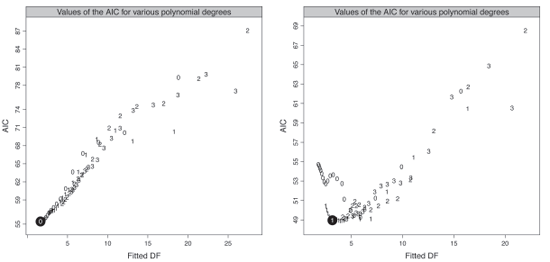
Values of the AIC criterion for various polynomial degrees, male population (left panel) and female population (right panel).
We select a constant and a linear fit with ν2=1.63 and 3.15 for the male and female population, corresponding to a window width of 41 and 31 observations respectively.
Having selected the optimal window width and polynomial degree, denoted h.Opt and P.Opt in the function below, we obtain the fitted probabilities of death by applying the improvement rates qx(t+1)/qx(t) derived from the reference with the following function:
> FctMethod4_2ndPart = function(d, e, qref, x1, x2, t1, t2, P.Opt, h.Opt){
+ Dx <- apply(as.matrix(d[x1 - min(as.numeric(rownames(d)))+1,]), 1, sum)
+ DxRef <- apply(as.matrix(as.matrix(e[x1 - min(as.numeric(rownames(e))) +
1,]) * qref[x1 - min(x2) + 1, as.character(t1)]), 1, sum)
+ QxtFitted <- predict(locfit(Dx ~ lp(x1, deg = P.Opt, nn = (h.Opt *
2 + 1) / length(x1), scale=1), ev = dat(), family = "poisson", link = "log",
kern = c("epan"), weights = c(DxRef))) * qref[x1 - min(x2) + 1,
as.character(min(t1):max(t2))]
+ colnames(QxtFitted) <- as.character(min(t1) : max(t2))
+ rownames(QxtFitted) <- x1
+ return(list(QxtFitted = QxtFitted, NameMethod = "Method4"))
+ }
9.3.5 Completion of the Tables: The Approach of Denuit and Goderniaux
Finally, we need to complete the tables. Due to the probable lack of data beyond a certain age, we do not have valid information to derive mortality at older ages. Actuaries and demographers have developed various techniques for the completion of the tables at older ages. In this chapter, we use a simple and efficient method proposed by Denuit & Goderniaux (2005). This method relies on the fitted one-year probabilities of death and introduces two constraints about the completion of the mortality table. It consists of fitting, by ordinary least squares, the following log-quadratic model:
logˆqx(t)=at+btx+ctx2+∈x(t),(9.2)
where ∈x(t)∼iid N(0,σ2), separately for each calendar year t at attained ages x* . Two restrictives conditions are imposed:
- First a completion constraint,
q130(t)=1,for all t.
Even though human lifetime does not seem to approach any fixed limit imposed by biological factors or other, it seems reasonable to accept the hypothesis that the age limit of end of life 130 will not be exceeded.
- Svalue associated to the likelihood ratio test (,
∂∂xqx(t)|x=130=0,for all t.
These constraints impose concavity at older ages in addition to the existence of a tangent at the point x=130 They lead to the following relation between the parameters at,bt and ct for each calendar year t:
at+btx+ct x2=ct(130−x)2,
for x=x*t,x*t+1,.... The parameters ct are estimated from the series {ˆqx(t),x=x*t,x*t+1,...} of calendar year t with Equation (9.2) and the constraints imposed. We implement the completion method in R as follows:
> CompletionDG2005 = function(q, x, y, RangeStart, RangeCompletion, NameMethod) {
+ x <- min(x) : pmin(max(x),100); RangeStart <- RangeStart - min(x)
+ RangeCompletion <- RangeCompletion - min(x)
+ CompletionValues <- matrix(, length(y), 3)
+ rownames(CompletionValues) <- y
+ colnames(CompletionValues) <- c("OptAge", "OptR2", "OptCt")
+ CompletionMat <- matrix(, RangeCompletion[2] - RangeCompletion[1] + 1,
length(y))
+ QxtFinal <- matrix(, RangeCompletion[2] + 1, length(y))
+ colnames(QxtFinal) <- y; rownames(QxtFinal) <- min(x) : 130
+ for(j in 1 : length(y)) {
+ R2Mat <- matrix(,RangeStart[2] - RangeStart[1] + 1, 2)
+ colnames(R2Mat) <- c("Age", "R2")
+ quadratic.q <- vector("list", RangeStart[2] - RangeStart[1] + 1)
+ for (i in 0 : (RangeStart[2] - RangeStart[1])) {
+ AgeVec <- ((RangeStart[1] + i) : (max(x) - min(x)))
+ R2Mat[i +1, 1] <- AgeVec[1]
+ FitLM <- lm(log(q[AgeVec + 1, j]) AgeVec + I(AgeVec~2))
+ R2Mat[i + 1, 2] <- summary(FitLM)$adj.r.squared
+ quadratic.q[[i + 1]] <- as.vector(exp(fitted(FitLM)))
+ }
+ if(any(is.na(R2Mat[,2])) == F){
+ OptR2 <- max(R2Mat[, 2], na.rm = T)
+ OptAge <- as.numeric(R2Mat[which(R2Mat[, 2] == OptR2), 1])
+ quadratic.q.opt <- quadratic.q[[which(R2Mat[, 2]==OptR2)]]
+ }
+ if(any(is.na(R2Mat[,2]))){
+ OptR2 <- NA; OptAge <- AgeVec[1]
+ quadratic.q.opt <- quadratic.q[[i +1]]
+ }
+ OptCt <- coef(lm(log(quadratic.q.opt) I((RangeCompletion[2] -
(OptAge : (max(x) - min(x))))~2) - 1))
+ CompletionVal <- vector(,RangeCompletion[2]-RangeCompletion[1]+1)
+ for (i in 0 : (RangeCompletion[2] - RangeCompletion[1])) {
+ CompletionVal[i + 1] <- exp(OptCt * (RangeCompletion[2] -
(RangeCompletion[1] + i))*2)
+ }
+ CompletionValues[j, 1] <- OptAge + min(x)
+ CompletionValues[j, 2] <- OptR2; CompletionValues[j, 3] <- OptCt
+ CompletionMat[, j] <- CompletionVal
+ QxtFinal[, j] <- c(q[1 : RangeCompletion[1], j], CompletionVal)
+ k <- 5; QxtSmooth <- vector(,2 * k + 1)
+ for(i in (RangeCompletion[1] - k) : (RangeCompletion[1] + k)){
+ QxtSmooth[1 + i - (RangeCompletion[1] - k)] <- prod(
QxtFinal[(i - k) : (i + k), j])*(1 / (2 * k + 1))
+ }
+ QxtFinal[(RangeCompletion[1] - k) : (RangeCompletion[1] + k), j]
<- QxtSmooth
+ }
+ return(list(CompletionValues = CompletionValues, CompletionMat =
CompletionMat, QxtFinal = QxtFinal, NameMethod = NameMethod))
+ }
As an illustration, the R2 and corresponding estimated regression parameters ct for the male and female population are displayed in Figure 9.5, left panel.
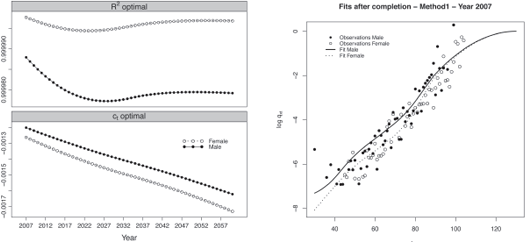
Regression parameters and fits obtained after the completion for the year 2007 with method 1.
We produced the figure with the following function, where the object CompletionMethodl has been obtained when fitting the completion procedure, see Section 9.5.5.
> PlotParamCompletion(CompletionMethod1, MyData$Param$Color)
The models capture more than 99.9% of the variance of the probabilities of death at high ages for both populations. The regression parameter ˆct represents the evolution of the mortality trends at high ages. We observe that the mortality at high ages decreases and the speed of improvement is relatively similar for both populations.
We keep the original ˆqx(t) for ages below 90 years old for both populations, and replace the annual probabilities of death beyond this age by the values obtained from the quadratic regression. The results obtained with method 1 for the calendar year 2007 are presented in Figure 9.5, right panel, for both populations.
The figure has been obtained with the function:
> FitPopsAfterCompletionLog(CompletionMethod1, MyData, 30 : 130,
 MyData$Param$Color, ” 2007”)
It should be noted that the completed part of the table is rather formal and is not validated.
9.4 Validation
The validation is assessed on three levels. This concerns the proximity between the observations and the model, the regularity of the fit, and the consistency and plausibility of the mortality trends.
9.4.1 First Level: Proximity between the Observations and the Model
The first level of the validation assesses the overall deviation with the observed mortality. It involves the SMR test proposed by Liddell (1984), the likelihood ratio test, and the Wilcoxon Matched-Pairs Signed-Ranks test. In addition, we find it useful to compare criteria measuring the distance between the observations and the models with the X2 applied by Forfar et al. (1988), the mean average percentage error (MAPE), and R2 applied by Felipe et al. (2002), as well as the deviance, the SMR, and the number of standardized residuals larger than 2 and 3.
The tests and quantities summarizing the overall deviation between the observations and the model are described in the following:
- x2
. This indicator allows one to measure the quality of the fit of the model. It is defined as
x2=∑(x,i)(Dx,t−Ex,tˆqx(t))2Ex,tˆqx(t)(1−ˆqx(t)) We will privilege the model having the lowest X2 .
- MAPE. This is a measure of accuracy of the fit to the observations. This indicator is the average of the absolute values of the deviations from the observations,
MAPE=∑(x,t)|(Dx,t/Ex,t−ˆqx(t))/(Dx,t/Ex,t)|∑(x,t)Dx,t×100.
It is a percentage and thus a practical indicator for the comparison. However, in the presence of zero observations, there will be divisions by zero, and these observations must be removed.
- R2
. The coefficient of determination measures the adequacy between the model and the observation. It is defined as the part of variance explained with respect to the total variance,
R2=1−((∑(x,t)(Dx,t/Ex,t−ˆqx(t))2∑(x,t)(Dx,t/Ex,t−(∑(x,t) (Dx,t/Ex,t)/n))2)
where n is the number of observations.
- The deviance. This a measure of the quality of the fit. Under the hypothesis of the number of deaths following a poisson law Dx,t∼P(Ex,t qx(t)), , the deviance is defined as
If Dx,t>1 and 0<Dx,t<Ex,t,Deviancex,t=
2(Dx,tln(Dx,tEx,tˆqx(t))+(Ex,t−Dx,t)ln(Ex,t−Dx,tEx,t−Lx,tˆqx(t)))
If Dx,t>0, Deviancex,t=2(Dx,tln(Dx,tEx,t˜qx(t) )−(Dx,t−Ex,t˜qx(t)))
- The likelihood ratio test. We can also consider the p-value associated to the likelihood ratio test (or drop-in deviance test). We seek, here, to determine if the fit corresponds to the underlying mortality law (null hypothesis Ho). The likelihood ratio test statistic, , is defined as
If is true, this statistic follows a law with the number of degrees of freedom equal to the number of observations n:
Hence, the null hypothesis is rejected if
where is the quantile of the distribution with n degrees of freedom. The p-value is the lowest value of the type I error for which we reject the test. We will privilege the model having the closest p-value to 1,
The SMR. This is the ratio between the observed and fitted number of deaths. If we consider that the number of deaths follows a poisson law
Hence, if SMR > 1, the fitted deaths are underestimated, and vice versa if SMR < 1.
- The SMR test. We can also apply a test to determine if the SMR is significatively different from 1, see Liddell (1984). We compute the following statistic:
where
If the SMR is not significatively different from 1 (null hypothesis Ho), this statistic follows a standard Normal law,
Thus, the null hypothesis H0 is rejected if
where is the quantile of the standard Normal distribution. The p-value is given by
We will seek to obtain the closest p-value to 1.
The Wilcoxon Matched-Pairs Signed-Ranks test. The framework of this test is very similar to the signs test. While the signs test only uses the information on the direction of the differences between pairs composed of the observed and fitted probabilities of death, the Wilcoxon test also takes into account the magnitude of these differences.
We test the null hypothesis H0 that the median between the difference of each pairs is null. We compute the difference between the observed and fitted probabilities of death, and rank them by increasing order of the absolute values, omitting the null differences. We assign to each non-zero difference its rank. We note the sum of the ranks of the differences strictly positive and negative, respectively. Finally, we note w, the maximum between the two numbers:
If the observed and fitted probabilities of death are equal, that is if H0 is true, the sum of the rank having a positive and negative sign should be approximatively equal. But if the sum of the ranks of positive signs differs largely from the sum of the ranks of the negative signs, we will deduce that the observed probabilities of death differ from the fitted ones, and we will reject the null hypothesis.
We can compute the statistic
If H0 is true, this statistic follows a standard Normal law,
Thus, the null hypothesis H0 is rejected if
where is the quantile of the standard Normal distribution. The p-value is given by:
We will seek to obtain the closest p-value to 1.
The Wilcoxon test uses the magnitude of the differences. The result may be different from the signs test that uses the number of positive and negative signs of the difference.
We implement the criteria and tests assessing the first level of validation in R as the following:
> TestsLevel1 = function(x, y, z, vv, AgeVec, AgeRef, YearVec, NameMethod){
+ quantities <- LRTEST <- matrix(, 4, 1)
+ SMRTEST <- WMPSRTEST <- matrix(, 5, 1)
+ RESID <- matrix(, 2, 1)
+ colnames(LRTEST) <- colnames(SMRTEST) <- colnames(RESID) <-
colnames(WMPSRTEST) <- colnames(quantities) <- NameMethod
+ rownames(LRTEST) <- c("Xi", "Threshold", "Hyp", "p.val")
+ rownames(SMRTEST) <- c("SMR", "Xi", "Threshold", "Hyp", "p.val")
+ rownames(RESID) <- c("Std. Res. > 2", "Std. Res. > 3")
+ rownames(quantities) <- c("Chi2", "R2", "MAPE", "Deviance")
+ rownames(WMPSRTEST) <- c("W", "Xi", "Threshold", "Hyp", "p.val")
+ xx <- x[AgeVec - min(as.numeric(rownames(x))) + 1, YearVec]
+ yy <- y[AgeVec - min(as.numeric(rownames(y))) + 1, YearVec]
+ zz <- z[AgeVec - min(as.numeric(rownames(z))) + 1, YearVec]
+ ##-------------- LR test
+ val.all <- matrix(, length(AgeVec), length(YearVec))
+ colnames(val.all) <- as.character(YearVec)
+ val.all[(yy > 0)] <- yy[(yy > 0)] * log(yy[(yy > 0)] / (xx[(yy > 0)] *
zz[(yy > 0)])) - (yy[(yy > 0)] - xx[(yy > 0)]) * (zz[(yy > 0)]
+ val.all[(yy ==0)] <- 2 * xx[(yy == zz)] * (zz[(yy == zz)] /
+ xi.LR <- sum(val.all)
+ Threshold.LR <- qchisq(1 - vv, df = length(xx))
+ pval.LR <- 1 - pchisq(xi.LR, df = length(xx))
+ LRTEST[1, 1] <- round(xi.LR, 2)
+ LRTEST[2, 1] <- round(Threshold.LR,2)
+ if(xi.LR <= Threshold.LR){LRTEST[3, 1] <- "H0"}
else {LRTEST[3, 1] <- "H1"}
+ LRTEST[4, 1] <- round(pval.LR, 4)
+ ##-------------- SMR test
+ d <- sum(yy); e <- sum(zz * xx); val.SMR <- d / e
+ if(val.SMR > -1){
+ xi.SMR <- 3 * d^(1/2) * (1 - (9 * d)"(- 1) - (d / e)^(- 1 / 3))}
+ if(val.SMR < -1){
+ xi.SMR <- 3 * (d + 1)^(1 / 2) * (((d + 1)/e)^(- 1 / 3) + (9 *
(d + 1))-(- 1) - 1)}
+ Threshold.SMR <- qnorm(1 - vv)
+ p.val.SMR <- 1 - pnorm(xi.SMR)
+ if(xi.SMR <= Threshold.SMR){SMRTEST[4, 1] <- "H0"}
else {SMRTEST[4,1] <- "H1"}
+ SMRTEST[1, 1] <- round(val.SMR, 4)
+ SMRTEST[2, 1] <- round(xi.SMR, 4);
+ SMRTEST[3, 1] <- round(Threshold.SMR, 4)
+ SMRTEST[5, 1] <- round(p.val.SMR, 4);
+ ## ------------- Wilcoxon Matched-Paris Signed-Ranks test
+ tab.temp <- matrix(, length(xx), 3)
+ tab.temp[, 1] <- yy / zz - xx
+ tab.temp[, 2] <- abs(tab.temp[, 1])
+ tab.temp[, 3] <- sign(tab.temp[, 1])
+ tab2.temp <- cbind(tab.temp[order(tab.temp[, 2]),], 1 : length(xx))
+ W.pos <- sum(tab2.temp[, 4][tab2.temp[, 3] > 0])
+ W.neg <- sum(tab2.temp[, 4][tab2.temp[, 3] < 0])
+ WW <- pmax(W.pos, W.neg)
+ Xi.WMPSRTEST <- (WW - .5 - length(xx) * (length(xx) + 1) / 4) /
sqrt(length(xx) * (length(xx) + 1) * (2 * length(xx) + 1) / 24)
+ Threshold.WMPSRTEST <- qnorm(1 - vv / 2)
+ p.val.WMPSRTEST <- 2 * (1 - pnorm(abs(Xi.WMPSRTEST)))
+ if(Xi.WMPSRTEST <= Threshold.WMPSRTEST){WMPSRTEST[4, 1] <- "H0"}
else {WMPSRTEST[4, 1] <- "H1"}
+ WMPSRTEST[1, 1] <- WW
+ WMPSRTEST[2, 1] <- round(Xi.WMPSRTEST, 4)
+ WMPSRTEST[3, 1] <- round(Threshold.WMPSRTEST, 4)
+ WMPSRTEST[5, 1] <- round(p.val.WMPSRTEST, 4)
+ ## ------------- Standardized residuals
+ val.RESID <- (xx - yy / zz) / sqrt(xx / zz)
+ RESID[1, 1] <- length(val.RESID[(abs(val.RESID)) > 2])
+ RESID[2, 1] <- length(val.RESID[(abs(val.RESID)) > 3])
+ ##-------------- chi^2, R2, MAPE
First level of validation, male population.
Method 1 |
Method 2 |
Method 3 |
Method 4 |
||
Standardized |
> 2
|
2 |
2 |
2 |
2 |
residuals |
> 3
|
0 |
1 |
1 |
1 |
|
53.13 |
57.79 |
55.82 |
51.81 |
|
|
0.7644 |
0.7312 |
0.7654 |
0 : 7554 |
|
MAPE (%) |
65.27 |
50.84 |
50.88 |
50.29 |
|
Deviance |
96.43 |
68.54 |
68.50 |
70.98 |
|
Likelihood |
|
48.22 |
34.27 |
34.25 |
35.49 |
ratio test |
p-value |
0.8826 |
0.9978 |
0.9978 |
0.9963 |
SMR test |
SMR |
0.7913 |
0.934 |
0.9681 |
0.9786 |
|
3.0098 |
0.8165 |
0.3573 |
0.2197 |
|
p-value |
0.0013 |
0.2071 |
0.3604 |
0.4131 |
|
Wilcoxon test |
W |
1154 |
1004 |
1014 |
1004 |
|
1.494 |
0.4166 |
0.4884 |
0.4166 |
|
p-value |
0.1352 |
0.6770 |
0.6252 |
0.6770 |
|
+ quantities[1, 1] <- round(sum(((yy - zz * xx)^2) / (zz * xx *
(1 - xx))), 2)
+ quantities[2, 1] <- round(1 - (sum((yy / zz - xx)^2) / sum((yy / zz -
mean(yy / zz))^2)), 4)
+ quantities[3, 1] <- round(sum(abs((yy / zz - xx) / (yy / zz))[yy > 0])
/ sum(yy > 0) * 100, 2)
+ quantities[4, 1] <- round(2*sum(val.all), 2)
+ RSLTS <- vector("list", 6)
+ RSLTS[[1]] <- LRTEST; RSLTS[[2]] <- SMRTEST; RSLTS[[3]] <- WMPSRTEST
+ RSLTS[[4]] <- RESID; RSLTS[[5]] <- quantities; RSLTS[[6]] <- NameMethod
+ names(RSLTS) <- c("Likelihood ratio test", "SMR test",
"Wilcoxon Matched-Pairs Signed-Ranks test", "Standardized residuals",
"Quantities", "NameMethod")
+ Return(RSLTS)
+}
We carry out the proposed tests and quantities. Tables 9.2 presents the results for the four methods and for the male population.
In a general manner, the four methods give acceptable results.
Besides the tests and quantities, the process of validation for the first level involves graphical analysis. It consists of representing graphically the fitted values against the observations for a given attained age or calendar year.
Figures 9.6 and 9.7 present the fitted probabilities of death in original and log scale obtained by the four methods for the age range [30, 90] and the calendar year 2007 for the male and female population, respectively. These graphics give a first indication about the quality of the fits. They have been produced using the following functions,
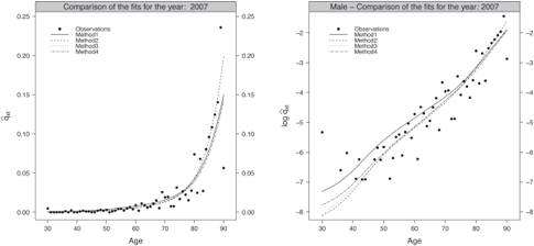
Fitted probabilities of death against the observations in original (left panel) and log scale (right panel), male population.
> ComparisonFitsMethods(ListOutputs, 2007, MyData$Male, AgeCrit, "Male", ColorComp, LtyComp)
> ComparisonFitsMethodsLog(ListOutputs, 2007, MyData$Male, AgeCrit, "Male", ColorComp, LtyComp)
where ListOutputs is the list of the objects OutputMethodl to OutputMethod4, see Section 9.5.3.
In conjunction with looking to the plots of the fits, we should study the residuals plots. We determine
Response residuals. ;
Pearson residuals. ;and
Deviance residuals. .
Such residual plots provide a powerful diagnostic that nicely complements the criteria. The diagnostic plots can show lack of fit locally, and we have the opportunity to judge the lack of fit based on our knowledge of both the mechanism generating the data and of the performance of the model.
We compute the residuals in R as follows:
> ResFct = function(x, y, z, AgeVec, YearVec, DevMat, NameMethod){
+ xx <- as.matrix(x)[AgeVec - min(as.numeric(rownames(x))) + 1, YearVec]
+ yy <- as.matrix(y)[AgeVec - min(as.numeric(rownames(y))) + 1, YearVec]
+ zz <- as.matrix(z)[AgeVec - min(as.numeric(rownames(z))) + 1, YearVec]
+ RespRes <- as.matrix(yy / zz - xx)
+ PearRes <- as.matrix((yy - xx * zz) / sqrt(xx * zz))
+ DevRes <- as.matrix(sign(yy / zz - xx) * sqrt(DevMat))
+ colnames(RespRes) <- colnames(PearRes) <- colnames(DevRes) <- YearVec
+ rownames(RespRes) <- rownames(PearRes) <- rownames(DevRes) <- AgeVec
+ Residuals <- list(RespRes, PearRes, DevRes, NameMethod)
+ names(Residuals) <- c("Response Residuals", "Pearson Residuals” ,
"Deviance Residuals", "NameMethod")
+ return(Residuals)
+ }
where the deviance is defined as
> DevFct = function(x, y, z, AgeVec, YearVec){
+ DevMat <- matrix(, length(AgeVec), length(YearVec))
+ colnames(DevMat) <- YearVec
+ xx <- as.matrix(x)[AgeVec - min(as.numeric(rownames(x))) + 1, YearVec]
+ yy <- as.matrix(y)[AgeVec - min(as.numeric(rownames(y))) + 1, YearVec]
+ zz <- as.matrix(z)[AgeVec - min(as.numeric(rownames(z))) + 1, YearVec]
+ DevMat[(yy > 0)] <- 2 * (yy[(yy > 0)] * log(yy[(yy > 0)] / (xx[(yy > 0)]
* zz[(yy > 0)])) - (yy[(yy > 0)] - xx[(yy > 0)]) * ((zz[(yy > 0)]
yy[(yy > 0)]) / (zz[(yy > 0)] - xx[(yy > 0)] * zz[(yy > 0)])))
+ DevMat[(yy == 0)] <- 2 * xx[(yy == 0)] * zz[(yy == 0)]
+ return(DevMat)
+ }
We superimposed a loess smooth curve on the response and Pearson residuals. These smooths help search for clusters of residuals that may indicate lack of fit. If the approach correctly models the data, no strong patterns should appear in the response and Pearson residuals. The plots of the residuals obtained by the four methods for the calendar year 2007 are displayed in Figure 9.7 for the male population. The figure has been obtained with:
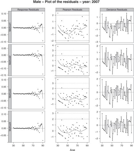
> ComparisonResidualsMethods(ListValidationLevel1, 2007, AgeCrit, "Male", ColorComp)
where ListValidationLevel1 is the list of the objects ValidationLevel1Method1 to ValidationLevel1Method4, see Section 9.5.4.
The Pearson residuals are mainly in the interval [—2, 2], indicating that the models adequately capture the variability of the dataset. The Pearson and response residuals obtained by fitting method 1 displays a more pronounced trend on the age range [30, 60] than the other ages. This indicates an inappropriate fit in this region. We can visualize this lack of fit in the deviance residuals where several successive residuals exhibit a negative sign. It illustrates that the data have been over-smoothed locally.
Finally, a classical step of the validation consists of comparing the observed and fitted deaths for a given attained age or calendar year over the common period of observation. Using the usual Normal approximation of a Poisson law, we can confront graphically the observed and fitted deaths as well as the lower and upper bounds of the pointwise confidence intervals.
Let suppose the following relation:
.
An approximation of the pointwise confidence intervals of is
,
where is the quantile of the Normal distribution.
> FittedDxtAndConfInt = function(q, e, x1, t1, ValCrit, NameMethod){
+ DxtFitted <- as.matrix(q[x1 - min(as.numeric(rownames(q))) + 1,
as.character(t1)] * e[x1 - min(as.numeric(rownames(l))) + 1, as.character(t1)])
+ DIntUp <- as.matrix(DxtFitted + qnorm(1 - ValCrit / 2) * sqrt(DxtFitted *
(1 - q[x1 - min(as.numeric(rownames(q))) + 1, as.character(t1)])))
+ DIntLow <- as.matrix(DxtFitted - qnorm(1 - ValCrit / 2) * sqrt(DxtFitted
* (1 - q[x1 - min(as.numeric(rownames(q))) + 1, as.character(t1)])))
+ DIntLow[DIntLow < 0] <- 0
+ colnames(DIntUp) <- colnames(DIntLow) <- colnames(DxtFitted) <-
as.character(t1)
+ rownames(DIntUp) <- rownames(DIntLow) <- rownames(DxtFitted) <- x1
+ return(list(DxtFitted = DxtFitted, DIntUp = DIntUp, DIntLow = DIntLow,
NameMethod = NameMethod))
+}
Figure 9.8 compares the observed and fitted deaths for the range [30, 90] in 2007 for the male population. The pointwise confidence intervals at 95% of the fitted deaths have been added to the plots. The figure have been produced with:
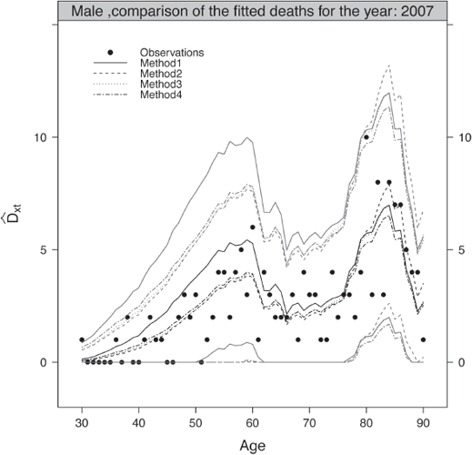
> ComparisonFittedDeathsMethods(ListValidationLevel1, 2007, MyData$Male, AgeCrit, "Male", ColorComp, LtyComp)
The observed deaths are within the bands of the theoretical pointwise confidence intervals at 95% over the age range considered. This indicates a correct representation of the reality by the male and female mortality tables.
9.4.2 Second Level: Regularity of the Fit
The second level of the validation assesses the regularity of the fit. It examines if the data have been over- or under-smoothed. It involves the number of positive and negative signs of the response residuals and the corresponding signs test, the number of runs, and the corresponding runs test used in Forfar et al. (1988) and Debóon et al. (2006).
The tests and quantities summarizing the regularity of the fit are described in the following:
Signs test. This is a nonparametric test that examines the frequencies of the signs changes of the difference between the observed and fitted probabilities of death. Under the null hypothesis Ho, the median between the positive and negative signs of this difference is null.
Let be the numbers of positive and negative signs, respectively, with ; the signs test statistic, , is defined by:
If H0 is true, this statistic follows a standard Normal law,
Thus, the null hypothesis H0 is rejected if
where is the quantile of the standard Normal distribution. The p-value is given by
.
We will seek to obtain the p-value closest to 1.
Runs test. This is a nonparametric test that determines if the elements of a sequence are mutually independent. A run is the maximal non-empty segment of the sequence consisting of adjacent equal elements. For instance, the following sequence composed of twenty elements,
consists of seven runs with four composed of + and three of -.
Under the null hypothesis H0, the number of runs of a sequence of n elements is a random variable whose conditional distribution given the numbers and of positive and negative signs, with is approximatively Normal, with:
The run text statistic, , is defined as
If H0 is true, this statistic follows a standard Normal law,
Hence, the null hypothesis H0 is rejected if
where is the quantile of the standard Normal distribution. The p-value is given by
.
We will seek to obtain the p-value closest to 1. This test is also called the Wald- Wolfowitz test.
> TestsLevel2 = function(x, y, z, vv, AgeVec, AgeRef, YearVec, NameMethod){
+ RUNSTEST <- matrix(, 7, 1)
+ SIGNTEST <- matrix(, 6, 1)
colnames(RUNSTEST) <- colnames(SIGNTEST) <- NameMethod
+ rownames(RUNSTEST) <- c("Nber of runs", "Signs (-)", "Signs (+)",
"Xi (abs)", "Threshold", "Hyp", "p.val")
+ rownames(SIGNTEST) <- c("Signs (+)", "Signs (-)", "Xi", "Threshold",
"Hyp", "p.val")
+ xx <- x[AgeVec - min(AgeVec) + 1, YearVec]
+ yy <- y[AgeVec - min(AgeRef) + 1, YearVec]
+ zz <- z[AgeVec - min(AgeRef) + 1, YearVec]
+ ##--------------------- Runs test
+ val.SIGN <- sign(yy / zz - xx)
+ fac.SIGN <- factor(as.matrix(val.SIGN))
+ sign.neg <- sum(levels(fac.SIGN)[1] == fac.SIGN)
+ sign.pos <- sum(levels(fac.SIGN)[2] == fac.SIGN)
+ val.RUNS <- 1 + sum(as.numeric(fac.SIGN[-1] !=
fac.SIGN[-length(fac.SIGN)]))
+ mean.run <- 1 + 2 * sign.neg*sign.pos / (sign.neg+sign.pos)
+ var.run <- 2 * sign.neg * sign.pos * (2 * sign.neg * sign.pos -
sign.neg - sign.pos) / ((sign.neg + sign.pos)"2 * (sign.neg + sign.pos - 1))
+ Threshold.RUNS <- qnorm(1 - vv/2)
+ xi.RUNS <- (val.RUNS - mean.run) / sqrt(var.run)
+ p.val.RUNS <- 2*(1-pnorm(abs(xi.RUNS)))
+ if(abs(xi.RUNS) <= Threshold.RUNS){RUNSTEST[6, 1] <- "H0"}
else {RUNSTEST[6,1] <- "H1"}
+ RUNSTEST[1, 1] <- val.RUNS
+ RUNSTEST[2, 1] <- sign.neg
+ RUNSTEST[3, 1] <- sign.pos
+ RUNSTEST[4, 1] <- round(abs(xi.RUNS), 4)
+ RUNSTEST[5, 1] <- round(Threshold.RUNS, 4);
+ RUNSTEST[7, 1] <- round(p.val.RUNS, 4)
+ ## -------------------- Sign test
+ SIGNTEST[1, 1] <- sign.pos
+ SIGNTEST[2, 1] <- sign.neg
+ xi.SIGN <- (abs(sign.pos - sign.neg) - 1) / sqrt(sign.pos + sign.neg)
Second level of validation, male population.
Method 1 |
Method 2 |
Method 3 |
Method 4 |
||
Signs test |
p-value |
25(36) 2.2804 0.2004 |
29(32) 0.2561 0.7979 |
30(31) 0 1 |
30(31) 0 1 |
Runs test |
Nber of runs
p-value |
32 0.3984 0.6903 |
36 1.2233 0.2212 |
34 0.6479 0.5171 |
34 0.6479 0.5171 |
+ Threshold.SIGN <- qnorm(1 - vv/2)
+ p.val.SIGN <- 2 * (1 - pnorm(abs(xi.SIGN)))
+ if(xi.SIGN <= Threshold.SIGN){SIGNTEST[5, 1] <- "H0"}
else {SIGNTEST[5, 1] <- "H1"}
+ SIGNTEST[3, 1] <- round(xi.SIGN, 4)
+ SIGNTEST[4, 1] <- round(Threshold.SIGN, 4)
+ SIGNTEST[6, 1] <- round(p.val.SIGN, 4)
+ RSLTS <- vector("list", 2)
+ RSLTS[[1]] <- RUNSTEST; RSLTS[[2]] <- SIGNTEST;
+ RSLTS[[3]] <- NameMethod
+ names(RSLTS) <- c("Runs test", "Signs test", "NameMethod")
+ return(RSLTS)
+ }
The results of tests carried out are presented in Table 9.3 for the four methods, for the male population.
From Table 9.3 we observe that, the regularity of the fit increases with the complexity of the models.
The two first levels of validation evaluate the fit according its regularity and the overall deviation from the past mortality. A satisfying fit, characterized by a homogeneous repartition of positive and negative signs of the response residuals and a high number of runs, should not lead to a significant gap with the past mortality, or vice versa. Accordingly, the two first levels of validation balance these two complementary aspects.
9.4.3 Third Level: Consistency and Plausibility of the Mortality Trends
The third level of the validation covers the plausibility and consistency of the mortality trends. It is evaluated by singles indices summarizing the lifetime probability distribution for different cohorts at several ages, such as the cohort life expectancies , median age at death and the entropy .
It also involves graphical diagnostics assessing the consistency of the historical and forecasted periodic life expectancy
In addition, if we have at our disposal the male and female mortality, we can compare the trends of improvement and judge the plausibility of the common evolution of the mortality of the two genders.
We refer to the concept of biological reasonableness proposed by Cairns et al. (2006b) as a means to assess the coherence of the extrapolated mortality trends. We ask the question: where are the data originating from, and based on this knowledge, what mixture of biological factors, medical advances, and environmental changes would have to happen to cause this particular set of forecasts?
It consists, initially, of obtaining the survival function calculated from the completed tables, see Section 9.3.5, resulting from the different approaches. From the survival function, we can derive a series of markers summarizing the lifetime probability distribution. We are interested in the survival distribution of cohorts for a given age at time t. Hence, we are working along the diagonal of the Lexis diagram. As a result, we can determine the mortality trends and compare the level and speed of improvement between the models.
We expose the indices summarizing the lifetime probability distribution in the following.
Survival function. The survival function of a cohort aged at time t measures the proportion of individuals of the cohort aged at time t being alive at age (or equivalently at time t + x). Under the condition , it writes
where the upper indices recalls that we are working along a diagonal of the Lexis diagram.
Cohort life expectancy. This is the partial life expectancy (over
years) of an individual of a cohort aged at time t. It is defined as
.
we obtain
Periodic life expectancy. This is the residual life expectancy (over years) of an individual aged x at time t. It is defined as
where the upper indices recalls that we are working along a vertical of the Lexis diagram.
Median age at death. The median age at death of an individual of a cohort aged at time t (over years), denoted , is the median of the lifetime probability distribution ,
.
Entropy. The entropy, , is the mean of weighted by (over years),
When the deaths become more concentrated, decreases. In particular, if the survival function has a perfect rectangular shape.
The single indices summarizing the lifetime probability distribution, presented above, are implemented in R as follows:
> FctSinglelndices = function(q , Age, t1, t2, NameMethod){
+ ## ------------- Survival functions
+ LSF <- floor(length(min(t1) : max(t2)) / 10) * 10 - 1
+ AgeSFMat <- min(Age) : (min(Age) + LSF)
+ NAgeSF <- AgeSFMat + 10
+ repeat{
+ if(max(NAgeSF) > 130){break}
+ AgeSFMat <- rbind(AgeSFMat, NAgeSF)
+ NAgeSF <- NAgeSF + 10
+ }
+ Start <- AgeSFMat[, 1]
+ NberLignes <- nrow(AgeSFMat) - length(Start[Start >= min(Age)])
+ AgeSFMat <- AgeSFMat[(NberLignes + 1) : nrow(AgeSFMat),]
+ Sx <- matrix(, ncol(AgeSFMat), nrow(AgeSFMat))
+ for(i in 1 : nrow(AgeSFMat)){
+ Sx[,i] <- SurvivalFct(q[AgeSFMat[i,] - min(Age) + 1,], 100,
AgeSFMat[i,])
+ }
+ ## ---------- Median age at death
+ print("Median age at death ...")
+ NameMedian <- vector(, nrow(AgeSFMat))
+ Rangelndices <- t(apply(AgeSFMat, 1, range))
+ for(i in 1 : nrow(AgeSFMat)){
+ NameMedian[i] <- paste("Med[", LSF+1, "_T_",RangeIndices[i,1],
"]", sep = "")
+ }
+ Sxx <- vector("list", nrow(AgeSFMat))
+ for(i in 1 : nrow(AgeSFMat)){
+ Sxx[[i]] <- vector("list", 2)
+ Sxx[[i]][[1]] <- Sxx[[i]][[2]] <- vector(, LSF * 100)
+ Temp <- GetSxx(t(Sx[, i]), c(1, LSF))
+ Sxx[[i]][[1]] <- Temp$a.xx
+ Sxx[[i]][[2]] <- Temp$Sxx
+ }
+ MedianAge <- matrix(, nrow(AgeSFMat), 1)
+ rownames(MedianAge) <- NameMedian
+ colnames(MedianAge) <- NameMethod
+ for (i in 1 : nrow(AgeSFMat)) {
+ MedianAge[i] <- Sxx[[i]][[1]][max(which(Sxx[[i]][[2]] >= 0.5)) +
1]
+ }
+ print(MedianAge)
+ ##---------------- Entropy
+ print("Entropy ...")
+ NameEntropy <- vector(, nrow(AgeSFMat))
+ for(i in 1 : nrow(AgeSFMat)){
+ NameEntropy[i] <- paste("H[", LSF + 1, "_T_", RangeIndices[i, 1],
"]", sep = "")
+ }
+ Entropy <- matrix(, nrow(AgeSFMat), 1)
+ colnames(Entropy) <- NameMethod
+ rownames(Entropy) <- NameEntropy
+ for(i in 1 : nrow(AgeSFMat)){
+ Entropy[i] <- round(- mean(log(Sx[,i]))/ sum(Sx[,i]), 4)
+ }
+ print(Entropy)
+ ## --------------- Cohort life expectancy for cohort in min(t1)
+ print(paste("Cohort life expectancy for cohort in",min(t1),"over",LSF+1,
years ..."))
+ NameEspGen <- vector(, nrow(AgeSFMat))
+ for(i in 1 : nrow(AgeSFMat)){
+ NameEspGen[i] <- paste(LSF+1,"_e_",RangeIndices[i,1],sep="")
+ }
+ CohortLifeExp <- matrix(, nrow(AgeSFMat), 1)
+ for(i in 1 : nrow(AgeSFMat)){
+ AgeVec <- AgeSFMat[i,]
+ CohortLifeExp[i] <- sum(cumprod(1 - diag(q[AgeVec + 1 - min(Age),
])))
+ }
+ colnames(CohortLifeExp) <- NameMethod
+ rownames(CohortLifeExp) <- NameEspGen
+ print(CohortLifeExpMale)
+ return(list(MedianAge = MedianAge, Entropy = Entropy, CohortLifeExp =
CohortLifeExp, NameMethod = NameMethod))
+}
From the survival function, we derive a series of markers summarizing the lifetime probability distribution. We are interested in the survival distribution of cohorts aged to 80 years old in 2007 over 50 years.
As an illustration, Table 9.4 presents the cohort life expectancies, the median age at death, and the entropy obtained with method 1 for the male population. Method 1 leads to the largest life expectancy. In consequence, the median age at death is the highest and the deaths are more concentrated.
In addition, if we have at our disposal the male and female mortalities, we can compare the trends of improvement and judge the plausibility of the common evolution of mortality of the two genders. For this purpose, we compare the male and female cohort life expectancies over 5 years.
> FctCohortLifeExp5 = function(q, Age, t1, t2, NameMethod){
+ AgeExp <- min(Age) : (min(Age)+4)
+ AgeMat <- matrix(, length(Age) - length(AgeExp) + 1, length(AgeExp))
+ AgeMat[1,] <- AgeExp
+ for (i in 2 : (length(Age) - length(AgeExp) + 1)){
+ AgeMat[i,] <- AgeMat[i - 1,] + 1
+ }
+ NameCohortLifeExp5 <- vector(, nrow(AgeMat))
+ for(i in 1 : nrow(AgeMat)){
+ NameCohortLifeExp5[i] <- paste(5, "_e_", AgeMat[i, 1], sep = "")
+ }
+ CohortLifeExp5 <- matrix(,length(Age) - length(AgeExp) + 1, length(t2) -
length(AgeExp) + 1)
+ colnames(CohortLifeExp5) <- as.character(min(t1) : (max(t2) - 4))
+ rownames(CohortLifeExp5) <- NameCohortLifeExp5
+ for (i in 1 : (length(t2) - length(AgeExp) + 1)){
+ for (j in 1 : nrow(AgeMat)){
+ AgeVec <- AgeMat[j,] + 1 - min(Age)
+ CohortLifeExp5[j, i] <- sum(cumprod(1 - diag(q[AgeVec,
i : (i + 4)])))
+}}
+ return(list(CohortLifeExp5 = CohortLifeExp5, NameMethod = NameMethod))
+ }
Figure 9.9 displays the ratio between the cohorts life expectancies (right panel) and between the fitted probabilities of death (left panel) of the two genders obtained with method 1.
The cohorts life expectancies of the female population are 8% larger than the male ones at 100 years old and 5% larger at 90 years old. The ratio between the cohorts life expectancies as well as the one between the fitted probabilities of death tend to get closer to 1 with the calendar year, indicating that the male mortality is improving more rapidly than the female, which seems plausible. However, after this age, the female mortality improvement increases more rapidly than the male mortality which does not sound coherent.
Finally, the third level of validation also involves graphical diagnostics assessing the consistency of the historical and forecasted periodic life expectancy.
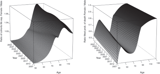
Ratio between the cohorts life expectancies (right panel) and the fitted probabilities of death (left panel) of the two genders obtained with method 1.
> FctPerLifeExp = function(q, Age, a, t1, t2, NameMethod){
+ AgeComp <- min(Age) : pmin(a, max(Age))
+ PerLifeExp <- matrix(, length(AgeComp), length(min(t1) : max(t2)))
+ colnames(PerLifeExp) <- as.character(min(t1) : max(t2))
+ rownames(PerLifeExp) <- AgeComp
+ for (i in 1 : (length(min(t1) : max(t2)))){
+ for (j in 1 : length(AgeComp)){
+ AgeVec <- ((AgeComp[j]) : max(AgeComp)) + 1 - min(Age)
+ PerLifeExp[j,i] <- sum(cumprod(1 - q[AgeVec, i]))
+ }
+}
+ return(list(PerLifeExp = PerLifeExp, NameMethod = NameMethod))
+}
To illustrate the consistency of the historical and forecasted periodic life expectancy,
Figure 9.10 compares the trends for the ages 55 and 70 obtained by the four methods for the male population.
The plots have been produced using:
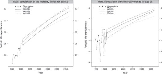
Comparison of the trends in periodic life expectancies for ages 55 and 70, male population.
> ComparisonTrendsMethods(ListValidationLevel3, 55, "Male", ColorComp, LtyComp)
> ComparisonTrendsMethods(ListValidationLevel3, 85, "Male", ColorComp, LtyComp)
The predicted periodic life expectancies obtained by the four methods adequately follow the observed trend. The trend derived from method 3 seems to deviate from the ones obtained by the other methods, leading to the slowest mortality improvement.
9.5 Operational Framework
In the following, we present an operational framework to implement the methodologies developed previously. The procedure is based on the software R and on package ELT (Experience Life Table) available on CRAN. Briefly, the procedure is as follows:
- i. We start by computing the number of deaths and exposition from the data line by line.
- ii. We import the reference table by gender.
- iii. We execute method 1.
- iv. We validate the resulting table with the first level of criteria. If the criteria assessing the proximity between the observation and the model are not satisfied, we turn to the following method of adjustment as it is useless to continue the process of validation.
- v. If the criteria assessing the proximity are satisfied, we continue the validation with the criteria of the second level assessing the regularity of the fit.
- vi. If the criteria assessing the regularity of the fit are satisfied, we complete the table at high ages using the procedure of Denuit & Goderniaux (2005).
- vii. We then pursue the validation with the criteria of the third level assessing the plausibility and coherence of the forecasted mortality trends. We can also turn to the next method to improve the fit at a cost of a somewhat greater complexity without degrading the results of the criteria corresponding to the first level. We repeat the step iii. to vii. with the following method.
9.5.1 The Package ELT
The package ELT allows one to implement the proposed methodology by the following functions.
- ReadHistory() to compute of the number of deaths, number of individuals, and exposure.
- AddReference() to import the reference of mortality.
- Method1() to execute the method 1, that is, applying the SMR to the probabilities of death of the reference.
- Method2() to execute the method 2, that is, a semi-parametric Brass-type relational model.
- Method3() to execute the method 3, that is, a Poisson GLM including the baseline mortality of the reference as a covariate and allowing interactions with age and calendar year.
- Method4A() to execute the first step of the method 4, the choice of the parameters for the local likelihood smoothing.
- Method4B() to execute the second step of the method 4, the application of the improvement rates derived from the reference.
- CompletionA() to execute the first step of the completion procedure, the choice of the age range.
- CompletionB() to execute the second step of the completion procedure.
- ValidationLevel1() to validate the methods according to the first level of criteria, that is, the proximity between the observations and the model.
- ValidationLevel2() to validate the methods according to the second level of criteria, that is, the regularity of the fit.
- ValidationLevel3() to validate the methods according to the third level of criteria, that is, the plausibility and coherence of the mortality trends.
In addition, the functions create the folder Results, which will be located in the current working directory, with the following subfolders:
- Excel where the files History.xlsx containing the number of deaths, number of individuals; and exposure of the population(s); Validation.xlsx containing the results of the level(s) of the validation, and FinalTables.xlsx storing the final mortality tables, will appear.
- Graphics, also decomposed according to
- — graphics of the observed statistics in the folder Data
- — graphics of the final tables in the folder FinalTables
- — graphics allowing one to judge the coherence of the mortality tables in the folder Validation
- — graphics allowing one to judge the regularity of the completed tables in the folder Completion
Finally, the package ELT uses the following dependencies, which need to be installed in advance:
- xlsx to export tables in Excel®
- locfit for the local likelihood smoothing
as well as the graphical packages
- lattice, grid, and latticeExtra
9.5.2 Computation of the Observed Statistics and Importation of the Reference
To obtain the observed number of deaths, number of individuals and exposure, we first need to read the data from the .csv file. For example:
> MyPortfolio = read.table(".../MyPortfolio.csv", header = TRUE, sep = colClasses = "character")
We then execute the function ReadHistory() with specifying the date of beginning and end of the period of observation as well as the format of the dates contained in the MyPortfolio.csv file.
> History <- ReadHistory(MyPortfolio = MyPortfolio, DateBegObs = "1996/01/01", DateEndObs = "2007/12/31", DateFormat = "0/Y/°/m/°/d", Plot = TRUE, Excel = TRUE)
By setting Excel = TRUE, we obtain an Excel file History.xlsx containing the observed statistics of the male and female population in the folder Results/Excel/ located in the current working directory.
In addition, by setting Plot = TRUE, we obtain graphics similar than Figures 9.2 and 9.3 in the folder Results/Graphics/Data.
Finally, we execute the function AddReference() to import the references of mortality. In this chapter, we use the national demographic projections for the French population over the period 2007-2060. Beforehand, we have extracted the references from the .csv files.
> ReferenceMale = read.table(".../QxtRefInseeMale.csv", sep = ",", header = TRUE)
> ReferenceMale <- ReferenceMale[,2:ncol(ReferenceMale)]
> ReferenceFemale = read.table(".../QxtRefInseeFemale.csv", sep = ",", header = TRUE)
> ReferenceFemale <- ReferenceFemale[,2:ncol(ReferenceFemale)]
> colnames(ReferenceMale) <- colnames(ReferenceFemale) <- 2007 : 2060
> rownames(ReferenceMale) <- rownames(ReferenceFemale) <- 30 : 95
> MyData <- AddReference(History = History, ReferenceMale = ReferenceMale, ReferenceFemale = ReferenceFemale)
9.5.3 Execution of the Methods
The approach involving one parameter is the simplest method considered, see Section 9.3.1. We specify the age range used to compute the SMR and execute the function Method1() to perform an adjustment with method 1.
> OutputMethod1 <- Method1(MyData = MyData, AgeRange =30 : 90, Plot = TRUE)
The second approach implies that the differences between the observed mortality and the reference can be represented linearly with two parameters through a semi-parametric Brass- type relational model, see Section 9_3_2. We specify the age range used to compute the parameters and execute the function Method2() to perform an adjustment with method 2.
> OutputMethod2 <- Method2(MyData = MyData, AgeRange =30 : 90, Plot = TRUE)
The third approach is a Poisson GLM including the baseline mortality of the reference as a covariate and allowing interactions with age and calendar year, see Section 9.3.3. We specify the age range used to compute the parameters of the Poisson GLMs and execute the function Method3() to perform an adjustment with method 3.
> OutputMethod3 <- Method3(MyData = MyData, AgeRange = AgeRange, Plot = TRUE)
The fourth approach involves a non-parametric smoothing of the periodic table by local likelihood and the application of the rates of mortality improvement derived from the reference. Its execution is in two steps, see Section 9.3.4. We specify the age range used to construct the periodic table and execute the function Method4A() to smooth the table with local likelihood technics.
> OutputMethod4PartOne <- Method4A(MyData = MyData, AgeRange =30 : 90, AgeCrit = AgeCrit, ShowPlot = TRUE)
By setting ShowPlot = TRUE, we obtain the graphical diagnostics used to select the smoothing parameters similar than Figure 9.4. The point corresponding to the minimum or a plateau after a steep descent of the criterion determines the optimal window width and polynomial degree, denoted by OptMale and OptFemale respectively for the male and female population. Finally, we execute the function Method4B() corresponding to the second step of the method to apply, to the smoothed periodic tables, the rates of mortality improvement derived from the references.
> OutputMethod4 <- Method4B(PartOne = OutputMethod4PartOne, MyData = MyData, OptMale = c(0, 20), OptFemale = c(1, 15), Plot = TRUE)
We obtain after the execution of each method, the fitted and extrapolated surfaces of mortality before the completion in the folder Results/Graphics/Completion by setting Plot = TRUE.
9.5.4 Process of Validation
We execute the function ValidationLevel1() to perform the validation with the criteria corresponding to the first level, see Section 9.4.1. We specify the age range used for the computation of the quantities and tests of the first and second levels as well as the critical value used by these tests.
> ValidationLevel1Method1 <- ValidationLevel1(OutputMethod = OutputMethod1,
MyData = MyData, AgeCrit =30 : 90, ValCrit = 0.05, Plot = TRUE, Excel = TRUE)
The execution of the function produces in the R console the values of the quantities and proposed tests used to assess the proximity between the observations and the model, see Table 9.2. These values are also recorded and stored in the Excel file Validation.xlsx in the folder Results/Excel/ if Excel = TRUE. As an example, the values obtained with method 1 for the male population are displayed below.
[1] "Validation: Level 1"
[1] "Male population: "
$'Likelihood ratio test'
Method1
Xi "69.71"
Threshold "80.23"
Hyp "H0"
p.val "0.2078"
$'SMR test'
Method1
SMR "1"
Xi "0.0265"
Threshold "1.6449"
Hyp "H0"
p.val "0.4894"
$'Wilcoxon Matched-Pairs Signed-Ranks test'
Method1
W "969"
Xi "0.1652"
Threshold "1.96"
Hyp "H0"
p.val "8688"
$'Standardized residuals'
Method1
Std. Res. >2 2
Std. Res. >3 0
$Quantities
Method1
Chi2 55.7900
R2 0.7201
MAPE 50.3200
Deviance 139.4300
We note that the null hypothesis H0 of the likelihood ratio test is verified, the fit corresponds to the underlying mortality law as well as the one of the Wilcoxon test, that is, the median of the difference of each pair composed of the observed and fitted probabilities of death is null.
The SMR is exactly equal to 1 as the model has the capacity to reproduce the observed number of deaths. The number of standardized residuals larger than 2 or 3, as well as the quantities, are indicative and provide a complement to the comparison of fits between the different methods.
In addition to the results of the tests of the first level, the validation involves graphical diagnostics such as the figures presented in Section 9.4.1 . Those graphics are available in the folder Results/Graphics/Validation if Plot = TRUE.
If the criteria of the first level are not satisfied, we turn to the following method as it is useless to continue the validation. If the criteria are satisfied, we pursue the second level of validation. As an example, we continue the validation with the criteria assessing the regularity of the fit; see Section 9.4.2. We execute the function ValidationLevel2():
> ValidationLevel2Method1 <- ValidationLevel2(OutputMethod = OutputMethod1,
MyData = MyData, AgeCrit = AgeCrit, ValCrit = 0.05, Excel = TRUE)
The execution of the script produces in the R console the values of the quantities and tests assessing the second level of validation; see Table 9.2. These values are also recorded and stored in the Excel file Validation.xlsx in the folder Results/Excel/ if Excel = TRUE is specified. In the following, we display the R output obtained for the male population after execution of method 1.
[1] "Validation: Level 2"
[1] "Male population: "
$'Runs test'
Method1
Nber of runs "32"
Signs (-) "36"
Signs (+) "25"
Xi (abs) "0.3984"
Threshold "1.96"
Hyp "H0"
p.val "0.6903"
$'Signs test'
Method1
Signs (+) "25"
Signs (-) "36"
Xi "1.2804"
Threshold "1.96"
Hyp "H0"
p.val "0.2004"
We note that the null hypothesis Ho of the runs test as well as the signs tests are verified.
If the criteria of the second level are not satisfied, we turn to the following method. If they are satisfied, we continue with the completion of the table at high ages. Having applied the completion method, see Sections 9.3.5 and 9.5.5, we have at our disposal completed tables until 130 years old. We execute the function ValidationLevel3() to assess the plausibility and coherence of the forecasted mortality trends.
> ValidationLevel3Method1 <- ValidationLevel3(FinalMethod = FinalMethod1, MyData = MyData, Plot = TRUE, Excel = TRUE)
The execution of the function produces singles indices summarizing the probability lifetime distribution for several cohorts; see Section 9.4.3 and Table 9.4. These values are also recorded and stored in the Excel file Validation.xlsx in the folder Results/Excel/ if Excel = TRUE is specified.
Single indices summarizing the lifetime probability distribution for cohorts of several ages in 2007 over 50 years, male population.
Method 1 |
Method 2 |
Method 3 |
Method 4 |
|
47.41 |
47.98 |
47.56 |
47.67 |
|
44.21 |
44.61 |
43.76 |
44.29 |
|
37.09 |
36.47 |
35.64 |
36.72 |
|
27.43 |
26.18 |
25.77 |
26.76 |
|
18.35 |
16.71 |
16.73 |
17.54 |
|
10.42 |
8.61 |
9.06 |
9.78 |
|
41.64 |
40.39 |
39.44 |
40.83 |
|
30.75 |
29.23 |
28.73 |
29.80 |
|
20.56 |
18.75 |
18.73 |
19.56 |
|
11.63 |
9.69 |
10.15 |
10.85 |
|
0.0011 |
0.0008 |
0.0010 |
0.0009 |
|
0.0027 |
0.0025 |
0.0030 |
0.0027 |
|
0.0093 |
0.0108 |
0.0121 |
0.0100 |
|
0.0400 |
0.0522 |
0.0539 |
0.0439 |
|
0.1782 |
0.2400 |
0.2356 |
0.1963 |
|
0.8511 |
1.1915 |
1.1038 |
0.9349 |
In addition, the validation involves graphical diagnostics such as the figures presented in Section 9.4.3, available in the folder Results/Graphics/Validation by setting Plot = TRUE.
9.5.5 Completion of the Tables
The completion of the tables is performed in two steps We first define the age range AgeRangeOpt in which the optimal starting age is determined and used to estimate the parameters ct; see Section 9.3.5. In addition, we have to initialize the age BegAgeComp from which we replace the fitted probabilities of death with the values obtained by the completion method. Then we execute the function CompletionA():
> CompletionMethodl <- CompletionA(OutputMethod = OutputMethodl, MyData = MyData, AgeRangeOptMale = c(80, 80), AgeRangeOptFemale = c(80, 80), BegAgeCompMale = 85, BegAgeCompFemale = 85, ShowPlot = TRUE)
By setting ShowPlot = TRUE,
the execution of this function produces the completed tables for the population(s) as well as graphics comparing the fit before and after the completion procedure; see Figure 9.5.
We then verify visually, in the second step, if the completed surface at high ages does not present breaks with the initial fit. We note, in Figure 9.5, that the junction between the fitted probabilities of death and the values obtained after the completion method appears relatively smooth.
If the completion is not satisfying, we modify the values AgeRangeOpt and BegAgeComp in the object ParamMortExp and repeat the execution of the function CompletionA(). If the completion is satisfying, we execute the function CompletionB() .
> FinalMethod1 <- CompletionB(ModCompletion = CompletionMethod1,
OutputMethod = OutputMethod1, MyData = MyData, Plot = TRUE, Excel = TRUE)
We obtain, after the execution of the function, the completed tables for the populations in the folder Results/Graphics/FinalTables, as well as the graphics comparing the fit before and after the completion procedure by calendar year in the folder Results/Graphics/Completionif Plot = TRUE. Finally, the final tables are stored in the Excel file FinalTables.xlsx in the folder Results/Excel/ if Excel = TRUE is specified.
1This chapter has benefitted substantially from the constructive comments of the working group Mortalité of the Institut des Actuaries. This research was supported by grants from BNP Paribas Cardif Chair Management de la modéelisation and the Institut des Actuaries.
2Available publicly here: www.ressources-actuarielles.net/gtmortalite.