CHAPTER 7
COMPUTATIONAL GEOMETRY AND FINITE ELEMENT ANALYSIS
Computational geometry methods such as Bezier, B-spline, and Non-Uniform Rational B-Splines (NURBS) are widely used in the design of engineering and physics systems (Dierckx, 1993; Farin, 1999; Piegl and Tiller, 1997; Rogers, 2001). At the design stage, the geometry of the systems is defined using computer-aided design (CAD) software. The CAD models then are converted to a finite element (FE) mesh to perform the analysis to determine deformations, stresses, and forces as the result of the applied loads. CAD systems use computational geometry methods that accurately define complex shapes and allow for efficient shape manipulation. These methods have many desirable features and share many of the properties required for the development of accurate analysis methods. Nonetheless, computational geometry methods are used primarily for the system geometric construction.
Because of the limitations of existing FE formulations and the fact that the geometric (i.e., kinematic) descriptions used in them are not equivalent to the geometric description used in CAD systems, there is a recent trend to use computational geometry methods as analysis tools. Although both FE and computational geometry methods are based on polynomial representations, many of the existing FE formulations distort the geometry because of the nature of the nodal coordinates selected. As a result, the geometry of the FE mesh used in the analysis can be different from the geometry defined in the CAD systems. This inconsistency makes the conversion of the CAD model to an analysis model difficult and costly and leads to analysis models that are not consistent with the CAD-geometry models. The two FE formulations discussed in Chapters 5 and 6 were developed to address and remedy this problem. The two formulations can be used as the basis for a successful integration of computer-aided design and analysis (I-CAD-A).
Both the FE floating frame of reference (FFR) formulation and the absolute nodal coordinate formulation (ANCF) (see Chapters 5 and 6) use a kinematic description that leads to a deformed shape that is invariant under an arbitrary rigid-body displacement. Because of this important property, both formulations lead to zero strains when the finite elements experience rigid-body displacements. Defining a geometry that is invariant under rigid body displacement is an important requirement for an accurate large-displacement analysis method. The FFR formulation, in particular, allows the use of finite elements that do not preserve the geometry to form an FE mesh that correctly describes rigid-body rotations. Using the concept of the intermediate element coordinate system, these finite elements can be assembled to form a mesh with geometry that is invariant under arbitrary rigid-body displacements.
In this chapter, computational geometry methods and their relationship to the FE formulations presented in this book are discussed. The limitations of using computational geometry methods as analysis tools are highlighted for an understanding of the potential use of these methods as alternatives to the FE formulations. As discussed herein, computational geometry methods – although they have many desirable features – have a rigid recurrence structure that can lead to higher-dimensional models, to the loss of flexibility provided by FE formulations in the selection of the basis functions, and to failure to capture certain types of geometric discontinuities that characterize many mechanical and structural systems. Nonetheless, a good grasp of computational geometry methods is important for understanding the limitations of some existing large-displacement FE formulations that have been widely used for decades.
7.1 GEOMETRY AND FINITE ELEMENT METHOD
As previously mentioned, computational geometry methods and FE formulations use polynomial representations. Nonetheless, in many structural FE formulations –particularly for beams, plates, and shells – the geometry is distorted because of the way the FE nodal coordinates are selected. Although rigid-body motion can be described in terms of trigonometric functions, as was shown in this book, the use of infinitesimal or finite rotations in the position field as nodal coordinates can lead to shapes that are not invariant under arbitrary rigid-body displacements. Similarly, finite rotations cannot be interpolated independently from the position field as is the case in some large-displacement FE formulations. The matrix of position-vector gradients uniquely defines the rotation and deformation fields. Therefore, independent interpolation of the rotation field leads to coordinate redundancy, as previously discussed. The limitations of existing FE formulations motivated researchers in the FE community to call for abandoning them and adopting computational geometry methods as analysis tools. However, computational geometry methods, as discussed in this chapter, have limitations as analysis tools: they can lead to higher-dimensional models, they do not provide the flexibility offered by the FE approach, and their recurrence formula fails to automatically capture certain types of geometric discontinuities, as previously mentioned.
ANCF description, on the other hand, is compatible with and has many of the desirable features offered by computational geometry methods. ANCF provides the flexibility of choosing the basis functions, does not have a rigid recurrence structure, and captures the geometric discontinuities that cannot be captured by computational geometry methods. For these reasons, ANCF finite elements allow for developing a simple interface between the CAD systems and analysis software.
Bezier Geometry
Computational geometry methods such as Bezier, B-spline, and NURBS used in CAD systems are based on polynomial representations (Dierckx, 1993; Farin, 1999; Piegl and Tiller, 1997; Rogers, 2001). The coefficients of the polynomials are replaced by coordinates of points, called control points, that form what is called a control polygon. Not all of the control points must lie on the curve or the surface; therefore, they are not necessarily material points as is the case in the FE representation. The use of control points that are not necessarily material points is a fundamental difference between computational geometry methods and FE formulations that use nodal coordinates to represent material points. Computational geometry methods are rooted in Bezier representation. Bezier representation, however, does not allow for domain discretization and for the use of piecewise polynomials; more complex shapes can be represented in Bezier geometry by increasing the polynomial order. Therefore, Bezier description, which does not allow for efficient shape manipulation, can be considered the counterpart of the Raleigh–Ritz analysis method, which uses modes that describe the deformation of the entire structure.
B-Spline Geometry
B-spline, in contrast, allows for domain discretization and the use of piecewise polynomials that define shapes over domain intervals (subdomains). B-spline geometry, therefore, is described by segments connected at points called breakpoints. For this reason, B-spline geometry description, which uses control points, can be considered the counterpart of the FE method. Being able to describe independently the geometry of segments over subdomains allows for efficient local shape manipulation because geometric changes can be made over small regions without affecting the geometry away from those regions. B-spline also uses the concept of knot vector and knot multiplicity, which allows for adjusting the degree of continuity at the breakpoints at which B-spline segments are connected. As the knot multiplicity at a given breakpoint decreases, the degree of continuity at that point increases. For example, a cubic B-spline curve representation with knot multiplicity of four at a point makes the curve discontinuous (C−1) at this point; knot multiplicity of three is associated with coordinate continuity (C0); knot multiplicity of two is associated with coordinate and gradient continuity (C1); and so on. B-spline representation is based on a recurrence structure that allows for automatically adjusting the degree of continuity by changing the knot multiplicity. Such a representation also allows for knot insertion and for adding control points to locally manipulate the geometry.
NURBS Geometry
There are shapes such as circular and conic segments the geometry of which cannot be described exactly using nonrational polynomials as those used in Bezier and B-splines; these shapes can be described exactly by using only rational functions (Dierckx, 1993; Farin, 1999; Piegl and Tiller, 1997; Rogers, 2001). NURBS geometry uses rational polynomials, allowing for exact geometric representation of circular and conic sections. NURBS geometry is based on a recurrence formula similar to that used in B-spline representation and it uses similar knot-vector and knot-multiplicity concepts. In Bezier, B-spline, and NURBS geometries, rigid-body displacement of a shape can be achieved by simply operating on the control points. A rigid-body transformation applied to the control points does not distort the geometry that undergoes the same transformation. For this reason, Bezier, B-spline, and NURBS geometry does not have the problems associated with some FE formulations in which the shape is not preserved under arbitrary rigid-body displacements.
7.2 ANCF GEOMETRY
As discussed in Chapter 5, the displacement field of ANCF finite elements is expressed in terms of position and gradient coordinates. This displacement field is invariant under arbitrary rigid-body displacements. In this section, it is shown that the ANCF kinematic description can be expressed in terms of the control points used in computational geometry methods. This alternate description can be used to establish the relationship among the ANCF, Bezier, B-spline, and NURBS descriptions. To this end, the three-dimensional ANCF two-node cable element that employs cubic interpolation is used. At each node, the element has six degrees of freedom, including three position coordinates and three components of one vector of position-vector gradients that remains tangent to the element centerline. The procedure developed in this section can be applied to other ANCF finite elements and generalized to the cases of surfaces and solids that are described using more general ANCF fully parameterized finite elements.
ANCF Element Geometry
In the case of the ANCF Euler–Bernoulli cable element, the global position vector r of an arbitrary point on the FE centerline can be defined using the element shape function matrix and the nodal coordinate vector as follows:
where S is the element shape function matrix expressed in terms of the element spatial coordinate x; e is the vector of nodal coordinates that consist of absolute nodal position coordinates and position coordinate gradients; and t is time. The element shape function matrix used in Equation 1 for the three-dimensional cable elements can be written as
where I is the identity matrix and si, i = 1, 2, 3, 4, are appropriate shape functions that can be introduced using polynomials or other geometric representations. The vector of the element nodal coordinates can be written as follows:
where superscripts A and B refer to the first and second nodes of the element, respectively; and the element nodal coordinate vector at node N is defined as follows:

The displacement field of this element can be defined using polynomial representation (described previously) as
In this equation, l is the length of the finite element, and ξ = x/l.
Control-Point Representation
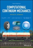
Whereas ANCF finite elements use gradients of absolute position vectors as nodal coordinates, a gradient vector always can be expressed in terms of the position vectors of two points divided by a scaling-length factor. Therefore, the ANCF geometric description presented in this section in terms of gradient vectors always can be converted to an equivalent geometric representation expressed solely in terms of position vectors of points that do not have to lie on the beam space curve or the plate and shell midsurface. As the finite element deforms, the location of these points will change with time. To demonstrate this coordinate transformation, the simple cable element defined previously is considered. For the cubic representation of Equation 5, one can define four points whose position vectors are defined by the vectors P0, P1, P2, and P3. Using these position vectors, the following coordinate transformation can be defined:

Substituting the coordinate transformation of this equation into Equation 5, one can show that the displacement field of the ANCF finite element can be written in terms of the point coordinates instead of the gradient coordinates as
The two representations of Equations 5 and 7 are equivalent and each can be used in the description of the geometry as well as the displacement, including deformations and rigid-body motion. Figure 1 is a graphical representation demonstrating the relationship between the gradient coordinates and point coordinates. In computational geometry, the points P0, P1, P2, and P3 are called control points. These points, which form the control polygon, do not have to represent material points. Equation 7, therefore, demonstrates how the geometric description of the ANCF finite elements can be expressed in terms of control points. The inverse relationship, in which the ANCF position and gradients coordinates are expressed in terms of the control points, can be obtained as explained in the following section. Such a relationship allows for converting CAD models to ANCF analysis meshes without geometry distortion.
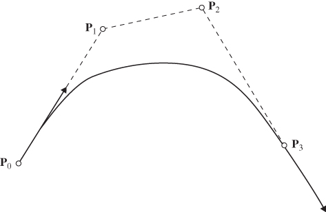
Figure 7.1 Gradients and control points
7.3 BEZIER GEOMETRY
Different methods can be used to represent polynomials, including the power basis and Bezier methods (Piegl and Tiller, 1997). Although the power basis and Bezier methods are equivalent, the Bezier method is more suited for shape manipulations and geometric modeling. In this section, it is shown that the Bezier geometry can be converted to ANCF geometry. This result is used to demonstrate that B-spline geometry can be converted to ANCF geometry, which can be proven because B-spline geometry is considered to consist of several Bezier segments.
A Bezier curve with m-degree is defined as (Piegl and Tiller, 1997)

In this equation, Si,m(ξ) are called the basis or blending functions, and the coefficients Pi are called the control points. The basis functions Si,m(ξ) are the m-degree Bernstein polynomials defined as
For example, in the case of a cubic curve (m = 3), one needs to evaluate S0,3, S1,3, S2,3, and S3,3. These four basis functions can be defined using Equation 9 as

Using these blending cubic functions and Equation 8, one can show that the cubic Bezier curve is defined by
This equation is the same as Equation 7 obtained using the ANCF geometry and the transformation from the gradient coordinates to the point coordinates defined by Equation 6. Equations 7 and 11 clearly demonstrate that the Bezier geometry can be converted to ANCF geometry using a simple linear transformation.
One can show that the Bernstein polynomials of Equation 9 have the following property (Piegl and Tiller, 1997):
with S−1,m−1 = Sm,m−1 = 0. Using this property, one can write

The Bernstein polynomials have many other interesting properties that are shared by the shape functions of many of the commonly used finite elements. Some of these properties are

Using the properties of the Bernstein polynomials, one can develop efficient algorithms, such as the deCasteljau algorithm, for the construction of Bezier curves (Piegl and Tiller, 1997).
The cubic Bezier function can also be expressed in terms of power-basis functions. This provides the following alternate form of Equation 7 or 11:
In this equation, 1, ξ, ξ2, and ξ3 are the power-basis functions. Bezier geometry also can be generalized to the case of surfaces, as discussed after introducing the B-spline geometry.
7.4 B-SPLINE CURVE REPRESENTATION
Bezier representation can be considered a special case of the more general B-spline representation. In the B-spline representation, several polynomial segments can be used, allowing for efficient shape and geometry manipulations. The B-spline geometry method, therefore, can be considered the counterpart of the FE analysis method, which allows geometric description over subdomains. A B-spline curve with p-degree is defined as (Dierckx, 1993; Farin, 1999; Piegl and Tiller, 1997; Rogers, 2001):

where Ni,p(u) are B-spline basis functions of degree p, Pi are the control points, and n is the number of control points. The B-spline basis functions Ni,p(u) are defined as

where ui = 0,1, 2,…, n + p + 1 are called the knots, which represent a nondecreasing sequence; that is, ui ≤ ui+1. The vector U = {u0 u1 … un+p+1} is called the knot vector. The knots do not have to be distinct; distinct knots are called breakpoints and define segments with nonzero length. Each nonzero knot span corresponds to a segment of the B-spline curve. The number of the nondistinct knots at a point is referred to as the knot multiplicity.
Control Points and Degree of Continuity
For a given polynomial order p, one can always define at a breakpoint p + 1 vectors. These vectors represent the position vector and its derivatives up to the pth derivative. For example, in the case of a cubic Bezier curve (p = 3), one can define r, ∂r/∂u, ∂2r/∂u2, and ∂3r/∂u3. Higher derivatives will be equal to zero. Therefore, in the case of two cubic Bezier segments i and j, one can have different conditions. If the two segments are not connected, the number of control points totals eight because each Bezier segment is represented using four (p + 1) control points. This is the case of C−1 continuity. In this case, all of the vectors r, ∂r/∂u, ∂2r/∂u2, and ∂3r/∂u3 that correspond to the first segment at the breakpoint are not related to the vectors r, ∂r/∂u, ∂2r/∂u2, and ∂3r/∂u3 that correspond to the second segment at this breakpoint. This case of C−1 continuity corresponds to the case of knot multiplicity of four (p + 1). If continuity is to be imposed on the position at the breakpoint at which the two segments are connected, one must have at the breakpoint the condition ri = rj, where i and j are the segment numbers. This algebraic equation, which ensures C0 continuity, can be used to write a control point of one segment in terms of the remaining control points. This leads to a reduction of the number of control points by one. This case of C0 continuity corresponds to knot multiplicity of three. Similarly, in the case of C1 continuity, two conditions are imposed at the breakpoint: the positions must be the same, ri = rj; and the gradients must be the same, (∂r/∂u)i = (∂r/∂u)j. These two vector algebraic equations allow for reducing the number of control points by two. This case corresponds to knot multiplicity of two in the case of cubic polynomials. Using a similar procedure, one can show that in the case of cubic polynomials, C2 continuity at a breakpoint corresponds to knot multiplicity of one and C3 continuity corresponds to knot multiplicity of zero. In the latter case of C3 continuity, the two segments blend together to form one larger cubic segment; four control points are eliminated, thereby reducing the number of control points for the newly created segment to four.
The concept of the knot multiplicity and the B-spline recurrence formula can be used to achieve automatically a higher degree of continuity by reducing the number of independent control points. Understanding the role of the knot multiplicity in B-spline representation is important when relating geometry methods to FE analysis methods that use the concept of nodes and degrees of freedom. If r + 1 is the number of knots in U, then in the B-spline geometry, one must have r = n + p + 1. This relationship can be verified easily starting with one Bezier segment. It is clear from this relationship that for a given polynomial degree p, reducing the knot multiplicity, to increase the degree of continuity, leads to a similar reduction in the number of control points, and increasing the knot multiplicity leads to a similar increase in the number of control points.
Illustrative Example
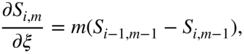
Figure 2 shows a cubic B-spline curve that has the six control points P0, P1, P2, P3, P4, and P5 and the knot vector U = {0 0 0 0 1 2 3 3 3 3} (Lan and Shabana, 2010). The number of segments in this example is s = 3 and the distinct breakpoints are ū0 = 0, ū1 = 1, ū2 = 2, and ū3 = 3. Note that if the knot vector has the form  , the B-spline curve reduces to a p-order Bezier curve; therefore, the Bezier curve can be considered a special case of the B-spline curve representation, as previously mentioned. At ū0 = 0, the knot multiplicity is four, which implies that there is no continuity condition imposed at this breakpoint, and r, ∂r/∂u, ∂2r/∂u2, and ∂3r/∂u3 are discontinuous. At the breakpoint ū1 = 1, the knot multiplicity is one and the curve is C2 continuous at this point. In this case, r, ∂r/∂u, and ∂2r/∂u2 are continuous, whereas the continuity of ∂3r/∂u3 is not ensured. The B-spline recurrence formula with the knot vector defined previously can be used to demonstrate this fact. The breakpoint ū2 = 2 has knot multiplicity of one; therefore, this point has continuity conditions similar to the breakpoint ū1 = 1. The breakpoint ū3 = 3 has knot multiplicity of four; therefore, this point has continuity conditions similar to ū0 = 0.

Figure 7.2 B-spline curve
Knot Insertion
By inserting knots into a B-spline knot vector, one can increase the number of control points as well as the knot multiplicity at selected points. For example, the S-shaped cubic B-spline curve shown in Figure 3, which has three segments, can be described by the knot vector U = {0 0 0 0 1 2 3 3 3 3} and the control points P0, P1, P2, P3, P4, and P5. Changing the knot vector to U = {0 0 0 0 1 1 1 2 2 2 3 3 3 3} by increasing the multiplicity at ū2 = 1 and ū2 = 2 to three reduces the degree of continuity at these breakpoints. At these points, the B-spline curve has C0 continuity, which ensures the continuity of the position vector only. Because the knot multiplicity is increased by two at two breakpoints, the number of control points increases by four. The corresponding control points for the new B-spline curve ![]() , and
, and ![]() also are shown in Figure 3. This B-spline curve, which ensures only C0 continuity at the inner breakpoints, is formed from three cubic Bezier curves that have the control points
also are shown in Figure 3. This B-spline curve, which ensures only C0 continuity at the inner breakpoints, is formed from three cubic Bezier curves that have the control points ![]() , and
, and ![]() . In fact, one can verify that any p-order C0 B-spline curve can be constructed using Bezier curves if the knot vector takes the form
. In fact, one can verify that any p-order C0 B-spline curve can be constructed using Bezier curves if the knot vector takes the form  . Decreasing the knot multiplicity at the inner breakpoints automatically increases the degree of continuity and eliminates the redundant control points. This process is built automatically in the powerful recurrence formula defined by Equations 16 and 17. Using these equations, one can also show that when the multiplicity at a breakpoint reduces to zero, two B-spline segments blend together to define one knot span with a length equal to the sum of the lengths of the two original segments. In addition to this powerful feature of the B-spline representation that provides the flexibility of easily changing the degree of continuity, the B-spline basis functions have unique desirable features such as the local support property, the nonnegativity, and the partition of unity (Dierckx, 1993; Farin, 1999; Piegl and Tiller, 1997; Rogers, 2001).
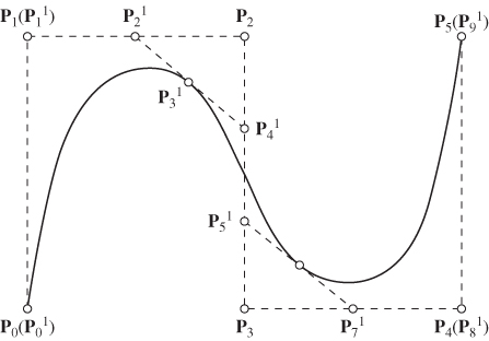
Figure 7.3 Knot insertion
Comparison with FE Formulations
Because of the problems associated with the kinematic description of existing FE formulations, computational geometry methods are being adopted as analysis tools. This led to a new research field known as isogeometric analysis, which is based on using CAD systems for both geometric modeling and analysis. As discussed in a subsequent section, computational geometry methods have serious limitations as analysis tools. These methods do not provide the flexibility offered by FE analysis methods and fail to capture certain types of discontinuities that define the geometric shapes of many mechanical and structural components. In the remainder of this section, the focus is on basic differences between the descriptions used by computational geometry and FE methods (Lan and Shabana, 2010).
The concept of nodes that represent material points on a curve or a surface is not used in B-spline geometry and other computational geometry methods; instead, computational geometry methods use control points that do not have to represent material points. The definition of nodes, is fundamental in the FE analysis. Different coordinate types such as positions, angles, gradients, curvatures, and stresses, among others, can be used as the nodal variables. The use of some of these coordinate types can impose restrictions on the geometric shapes that can be assumed by the finite elements. In fact, some of the conventional finite elements do not preserve the shapes of the finite elements under an arbitrary rigid-body transformation, as previously discussed. The kinematic description used for these elements, therefore, is not equivalent to the descriptions used by computational geometry methods such as the B-spline representation. For this reason, the geometry of the FE mesh used in the analysis in the reference configuration is not always identical to the geometry created in CAD systems. B-spline geometry, however, can always be converted to ANCF geometry using simple linear transformation. The converse is not always true, as demonstrated later in this chapter.
Another fundamental difference between the geometric descriptions used in the FE and computational geometry methods is the domain definition. Most FE formulations use the domain in the reference configuration such as the undeformed-length or cross-sectional dimensions of a beam to carry out the integrations required to formulate the FE inertia and stiffness forces. The concept of reference configuration or element domain as used in FE analysis is not used in computational geometry methods. Therefore, it is important to address this issue to successfully convert the B-spline geometry to an FE mesh with the exact geometric properties as that developed in a CAD system (Lan and Shabana, 2010).
7.5 CONVERSION OF B-SPLINE GEOMETRY TO ANCF GEOMETRY
One method for the integration of CAD and analysis is to establish an efficient interface that can be used to convert the CAD model to an FE mesh that has geometry identical to the model created in the CAD system. This was not possible in the past because conventional structural finite elements such as beams, plates, and shells are based on a kinematic description that is not consistent with the description used by computational geometry methods. This problem, however, can be solved by using ANCF finite elements because B-spline geometry can always be converted to an ANCF representation using simple linear transformation.
How to convert a Bezier curve representation to ANCF representation is shown in this chapter (Sanborn and Shabana, 2009). Because a B-spline curve can be represented as a series of connected Bezier curves, the curves can be converted to ANCF cable elements. This demonstrates that ANCF cable elements can have geometry identical to that of the original B-spline curve representation. In the case of the ANCF cable elements, the global position vector r of an arbitrary point on the FE centerline can be defined using the element shape functions and the nodal coordinate vector as r(x, t) = S(x)e(t), where S is the element shape function matrix expressed in terms of the element spatial coordinate x; ![]() is the vector of nodal coordinates that consist of absolute position and gradient coordinates of the first and second nodes of the element (denoted, respectively, as A and B); and t is time. For the three-dimensional cable elements, the shape function matrix can be written as S = [s1I s2I s3I s4I], where I is the identity matrix and si, i = 1, 2, 3, 4, are shape functions defined as
is the vector of nodal coordinates that consist of absolute position and gradient coordinates of the first and second nodes of the element (denoted, respectively, as A and B); and t is time. For the three-dimensional cable elements, the shape function matrix can be written as S = [s1I s2I s3I s4I], where I is the identity matrix and si, i = 1, 2, 3, 4, are shape functions defined as

In this equation, l is the FE length, and ξ = x/l.
The cubic Bezier curve control points P0, P1, P2, and P3 can be written in terms of the ANCF nodal coordinates using the following equation (see also Equation 6):

Substituting this equation into the Bezier curve representation, one can obtain ANCF representation that has identical geometry to that represented by the B-spline recurrence formula. Alternatively, using Equation 6, one can show that the kinematics of the ANCF cable element can be expressed in terms of the cubic Bezier curve control points as (Lan and Shabana, 2010):

where the relationship between the ANCF shape functions and the Bernstein polynomials S0,3, S1,3, S2,3, and S3,3 is defined as

To convert a B-spline curve into an ANCF cable element, an assumed element length l should be defined first. In this case, the B-spline curve that is represented with a series of ANCF cable elements also has a domain that is the sum of all of the assumed element lengths. This domain is defined as ![]() , where L is the assumed domain of the B-spline curve, s is the number of segments, and li is the length of the ith ANCF cable element in the reference undeformed configuration. As described by Lan and Shabana (2010), this domain can be used to define consistently the gradients and derivatives when converting B-spline geometry to ANCF FE representation.
, where L is the assumed domain of the B-spline curve, s is the number of segments, and li is the length of the ith ANCF cable element in the reference undeformed configuration. As described by Lan and Shabana (2010), this domain can be used to define consistently the gradients and derivatives when converting B-spline geometry to ANCF FE representation.
7.6 ANCF AND B-SPLINE SURFACES
Fully parameterized planar ANCF finite elements and all spatial ANCF finite elements, including gradient-deficient elements, preserve the geometry under an arbitrary rigid-body displacement. This important condition, which also is satisfied by computational geometry methods, ensures that B-spline geometry can always be converted to ANCF FE mesh that has identical geometry. Nonetheless, ANCF geometry cannot always be converted to B-spline geometry because of the structure of the B-spline recurrence formula. In this section, fundamental differences between the ANCF and B-spline geometric representations are discussed. To this end, surface geometry in fully parameterized planar ANCF beam elements and gradient-deficient spatial-plate elements is used.
B-Spline Surfaces
B-spline surfaces are defined using the product of B-spline base functions, two parameters, and two knot vectors. B-spline surfaces can be defined in the following parametric form (Piegl and Tiller, 1997):

where u and v are the parameters; Ni,p(u) and Nj,q(v) are B-spline basis functions of degrees p and q, respectively; and Pi,j are a set of bidirectional net of control points. The B-spline basis functions Ni,p(u) are defined as

where ui,j = 0, 1, 2,…, n + p + 1 are called the knots and ui ≤ ui+1. The vector U = {u0, u1…un+p+1} is called the knot vector associated with the u parameter. Similar definitions can be introduced for Nj,q(v) with another knot vector V = {v0 v1 · · · vm+q+1}. Note that the orders of the polynomials in the u and v directions can be different; for example, a cubic interpolation can be used along u, whereas a linear interpolation can be used along v. As in the case of B-spline curves, the knots of B-spline surfaces do not have to be distinct; distinct knots are called breakpoint and define surface segments with nonzero dimensions. The number of the nondistinct knots in U and V at a point is referred to as the knot multiplicity associated, respectively, with the parameters u and v at this point. At a given breakpoint, the multiplicity associated with u can be different from the multiplicity associated with v, allowing for different degrees of continuity for the derivatives with respect to u and v. For cubic Ni,p (p = 3), C0, C1, or C2 conditions correspond, respectively, to knot multiplicity of three, two, and one; whereas in the case of linear interpolation of Nj,q, the highest continuity degree that can be demanded is continuity of the gradients. When zero multiplicity is used at a breakpoint, the segments blend together at this point.
In B-spline surface representation, there is a relationship among the polynomial degree, the number of knots, and the number of control points. This relationship must be fully understood if B-spline geometry is used as an analysis tool. If r + 1 is the number of knots in U and s + 1 is the number of knots in V, then in B-spline geometry, one must have
As in the case of B-spline curves, these formulas imply that for a given polynomial order, if the number of knots decreases, the number of control points that defines the number of degrees of freedom used in the analysis must also decrease. This also can be equivalent to increasing the degree of continuity because eliminating a control point can be the result of imposing algebraic equations that relate the derivatives at a certain breakpoint.
From the bidirectional structure used in Equation 22, a surface segment that has cubic interpolation along u(p = 3, n = 3, r + 1 = 8) and a linear interpolation along v(q = 1, m = 1, s + 1 = 4) should have (n + 1) × (m + 1) = 8 control points; this is true regardless of whether the surface is two- or three-dimensional. Manipulation of the B-spline surface defined by Equation 22 shows that these eight control points are the result of using the alternate basis set 1, u, v, uv, (u)2, (u)2v, (u)3, (u)3v. That is, B-spline representation and the formulas of Equation 24 do not allow for the use of the basis set 1, u, v, uv, (u)2, (u)3, which can be used effectively to develop a shear deformable beam model. If a cubic interpolation is used for both u and v (case of thin plate), the B-spline representation will require 16 control points because the expansion must include all terms (u)k (v)l; k, l = 0, 1, 2, 3, regardless of whether the shape of deformation of the plate is simple or complex; one must follow strictly the B-spline rigid structure. This can be a disadvantage in the analysis because such a geometric representation can increase unnecessarily the dimensions of the model and lead to the loss of flexibility offered by the FE method or modal analysis techniques. Another important and interesting issue regarding the use of B-spline as an analysis tool is capturing discontinuities, which is discussed later in this chapter.
ANCF Surfaces
Whereas B-spline geometry always can be converted to ANCF geometry, the converse is not true. ANCF geometry does not impose restrictions on the basis functions that must be included in the interpolating polynomials. This allows for developing finite elements that have a small number of nodal coordinates as compared to those developed using the B-spline representation. Furthermore, ANCF geometry can be used to model both structural and nonstructural discontinuities, whereas the rigid B-spline recurrence representation cannot be used to model structural discontinuities in a straightforward manner, as discussed in the following section.
A basic difference between ANCF and B-spline geometries is demonstrated in this section using a planar-beam example. The displacement field of the shear deformable beam used can be written as r(x1, x2) = S(x1, x2) e(t), where x1 and x2 are the element spatial coordinates, t is time, S is the element shape function matrix, and e is the vector of the element nodal coordinates. The shape function matrix for the element considered in this section is defined as
where the shape functions si, i = 1, 2, …, 6, are defined as (Omar and Shabana, 2001):

In this equation, ξ = x1/l, and η = x2/l. ANCF finite elements use gradient vectors as nodal coordinates. For the element used in this section, the vector of nodal coordinates is defined as
where superscript k, k = 1, 2, indicates variables evaluated at node k of the element. The element defined by the preceding equations is based on a cubic interpolation for x1 and a linear interpolation for x2.
The finite element described in this section is an example of ANCF elements that cannot be converted to B-spline representation. This element is based on a polynomial expansion that does not have the two basis functions (x1)2 x2 and (x1)3 x2. These terms can be systematically included in ANCF geometry by adding nodal coordinates, which allows for converting B-spline representation to ANCF representation. Similar comments apply to ANCF thin-plate elements that do not require including all of the basis functions (x1)k (x2)l; k, l = 0, 1, 2, 3. This flexibility offered by ANCF geometry allows for developing finite elements that have a smaller number of nodal coordinates compared to those elements developed by B-spline geometry.
7.7 STRUCTURAL AND NONSTRUCTURAL DISCONTINUITIES
In this section, two types of discontinuities explain another fundamental difference between ANCF and B-spline geometries: structural and nonstructural discontinuities. In the case of structural discontinuity, there is no relative rigid-body motion at the discontinuity node; all of the relative degrees of freedom are deformation degrees of freedom. An example of structural discontinuity is at point C in Figure 4. At the structural-discontinuity node, in the case of the planar system shown in Figure 4, there is only one state of strains. Nonstructural discontinuity, conversely, allows for relative rigid-body rotation. At points O and B in Figure 4, there can be two different states of strains because of the rigid-body mode. Although both structural and nonstructural discontinuities can be classified as C0, they are fundamentally different from the analysis perspective because they lead to two completely different joint models that have different degrees of freedom. Only one of these types of discontinuities can be captured by the B-spline recurrence formula, whereas the other cannot be captured. Both, however, can be captured by ANCF finite elements.

Figure 7.4 Structural and nonstructural discontinuities
B-Spline Model
As previously mentioned, reducing the knot multiplicity by one at a curve breakpoint leads to C0 continuity and to the elimination of one control point. This is equivalent to the multibody system (MBS) pin-joint-constraint definition in planar analysis and to the MBS spherical-joint definition in spatial analysis. This type of C0 continuity captured by B-spline is of the nonstructural-discontinuity type that leads to a rigid-body mode and to a nonunique state of the strain at the discontinuity node. The B-spline recurrence formula structure leads automatically to this type of discontinuity. The structural discontinuity, although it is also of the C0 type, requires additional algebraic equations to define a unique strain state by eliminating the relative rotation at the joint definition point. These algebraic equations can be used to eliminate other control points and such elimination is not embedded in the rigid B-spline geometry representation. Only one type of C0 continuity can be described using B-spline formula; reducing the knot multiplicity by one in B-spline representation does not capture structural discontinuity. More fundamental problems are encountered when B-spline surfaces are considered in MBS applications as explained in the literature (Yu and Shabana, 2015).
ANCF Model
One can show that ANCF finite elements describe both structural and nonstructural discontinuities. Nonstructural discontinuities that allow for large rigid-body rotations can be described using a C0 model obtained by imposing constraints only on the position coordinates. For example, if two elements i and j are connected by a pin joint at a node, one can apply the algebraic equations ri = rj at this node. These algebraic equations can be imposed at a preprocessing stage to eliminate the dependent variables and to define an FE mesh that has a constant mass matrix and zero Coriolis and centrifugal forces, despite the finite rotations allowed between the finite elements of the mesh. As previously mentioned, nonstructural discontinuities also can be described using B-spline geometry by reducing the knot multiplicity by one at the joint node. In the case of nonstructural discontinuities, no constraints are imposed on the gradient vectors; therefore, the state of strain is not unique at the joint node. Each of the Lagrangian strains ![]() ,
, ![]() , and
, and ![]() has two values at the joint node: one defined on element i and the other on element j. Here,
has two values at the joint node: one defined on element i and the other on element j. Here, ![]() ,
, ![]() .
.
The concept of degrees of freedom widely used in mechanics is not considered in developing the recurrence relationships on which B-spline and NURBS geometry are based. This represents another serious limitation when these computational geometry methods are used as analysis tools, which is evident by the fact that B-spline geometry cannot describe structural discontinuities. As previously mentioned, this type, although it is of the C0 continuity type, requires imposing additional gradients constraints, which cannot be captured by the B-spline recurrence formula because they require the elimination of additional vectors. In the case of B-spline, C0 continuity is achieved by reducing the knot multiplicity by one, which eliminates one control point leading to the definition of a pin joint (nonstructural discontinuity). ANCF geometry, conversely, allows for imposing constraints on the gradients using the tensor transformation (∂r/∂x) = (∂r/∂y)A, where ![]() and
and ![]() are two sets of coordinate lines and A is the matrix of coordinate-line transformation. Using this tensor-gradient transformation, the structural discontinuities can be modeled systematically using ANCF finite elements, as described in the literature (Shabana and Mikkola, 2003; Shabana, 2011).
are two sets of coordinate lines and A is the matrix of coordinate-line transformation. Using this tensor-gradient transformation, the structural discontinuities can be modeled systematically using ANCF finite elements, as described in the literature (Shabana and Mikkola, 2003; Shabana, 2011).
PROBLEMS
-
1 Explain the differences between Bezier and B-spline geometry representations.
-
2 Discuss the similarities and differences between the B-spline and NURBS representations.
-
3 Starting with a cubic polynomial, derive the cubic Bezier curve in terms of the control points and define the basis functions of Equation 10.
-
4 Explain the basic differences between the B-spline and finite element representations.
-
5 For a cubic Bezier curve, derive the relationship between the control points and the nodal coordinates of the ANCF cable element.
-
6 Explain how the degree of continuity can be adjusted when using the B-spline geometry. In B-spline geometry, can continuity be imposed on the gradients without having position continuity? Provide an explanation.
-
7 Explain the meaning of the knot multiplicity. In the case of cubic B-spline curve, explain the meaning of knot multiplicity of 1, 2, 3, and 4. Give examples to show the relationship between the knot multiplicity and the number of the B-spline control points.
-
8 Explain why B-spline geometry can always be converted to ANCF geometry, while the converse is not true. Give an example to support the argument made.
-
9 Give an example of a cubic B-spline surface and explain how this surface can be converted to an ANCF finite element.
-
10 Explain the differences between structural and nonstructural discontinuities. Give examples to explain these differences.