
CAM system for articulated-type industrial robot
Abstract:
In this chapter, a CAM system for an articulated-type industrial robot RV1A is proposed in order to raise the relationship between a CAD/CAM and industrial robots spread to industrial manufacturing fields. A simple and flexible CAM system is designed from the viewpoint of the cooperation between CL data and robotic servo system. The CAM system required for an industrial robot is realized as an integrated system including not only a conventional main-processor of CAM but also a robotic servo system and kinematics, so that the RV1A can be directly controlled without any conventional teaching process. The basic design of the CAM system and experimental results are shown using the industrial robot RV1A. The effectiveness is demonstrated through a trajectory following a control experiment along multi-axis CL data consisting of position and orientation components and passive force control experiments.
3.1 Background
Many studies focusing on teaching of industrial robots have already been conducted. The authors developed a joystick teaching system for a polishing robot to safely obtain suitable orientation data of a sanding tool attached to the tip of robot arm [26, 27, 82]. Maeda et al. proposed a simple teaching method for industrial robots by human demonstration. The proposed automated camera calibration enabled labor-saving teaching and compensated the absolute positional error of industrial robots [28]. Also, Kushida et al. proposed a method of force-free control for industrial articulated robot arms. The control method was applied to the direct teaching of industrial articulated robot arms, in which the robot arm was directly moved by human force [29]. Furthermore, Sugita et al. developed two kinds of teaching support devices, i.e., a three-wire type and an arm-type, for a deburring and finishing robot. The validity of the proposed devices was verified through experiments using an industrial robot [30]. As for off-line teaching, Ahn and Lee proposed an off-line automatic teaching method using vision information for robotic assembly task [31]. Moreover, a CAD-based off-line teaching system was proposed by Neto et al., which allows users with basic CAD skills to generate robot programs off-line, without stopping the production by using a robot [32]. Besides, Ge et al. showed a basic transformation from CAD data to position and orientation vectors for a polishing robot [33].
As surveyed above, several promising teaching systems for industrial robots have been already developed for each task. However, it seems that a CAM system from the viewpoint of a robotic servo system has not been sufficiently discussed yet. In this book, it is assumed that a CAM system includes an important function which allows an industrial robot to be accurately controlled along cutter location data (CL data) consisting of position and orientation components. Another important point is that the proposed CAM system has a high applicability to other industrial robots whose servo systems are technically opened to engineering users. At the present stage, the relationship between CAD/CAM and industrial robots is not well established compared to NC machine tools widely used in manufacturing industries. In general, the main-processor of CAD/CAM calculates CL data according to each model’s shape and cutting strategy, then the post-processor produces suitable numerical control data (NC data) for an NC machine tool which is actually used. The controller of an NC machine tool sequentially deals with NC data and accurately controls the position and the orientation of the main head as an example.
Thus, it seems that CAM system for NC machine tools is a mature one. On the other hand, a CAM system for industrial robots has not yet been sufficiently considered and standardized. That is the reason why, when an industrial robot is applied to a task, the required position and orientation data are acquired by on-line and/or off-line teaching systems instead of CAM systems in almost all cases.
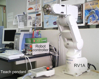
In this book, a CAM system for an articulated-type industrial robot RV1A shown in Fig. 3.1 is described from the viewpoint of a robotic servo controller. It is defined here that a CAM system includes an important function which allows an industrial robot to move along CL data consisting of position and orientation components. Another important point is that the proposed CAM system has a high applicability to other industrial robots whose servo systems are technically opened to end-user engineers. The CAM system works as a flexible interface between CAD/CAM and industrial robots. At the present stage, the relationship between CAD/CAM and industrial robots is not well established compared to NC machine tools widely used in manufacturing industries. Generally, the main-processor of CAD/CAM generates CL data according to each model shape and cutting conditions, then the post-processor produces suitable NC data for an NC machine tool which is actually used. The controller of NC machine tool sequentially deals with NC data and accurately controls the positions of main head and the angles of other axes. Thus, CAM systems for NC machine tools are already established. On the other hand, CAM systems for industrial robots have not been sufficiently considered and standardized yet. A teaching pendant is used in almost all cases to obtain position and orientation data from the arm tip before an industrial robot can work well. Here, in order to improve the relationship between conventional CAD/CAM and an industrial robot, a simple and flexible CAM system is proposed. The basic design of the CAM system and an experimental result are shown.
3.1 Desired trajectory
3.2.1 Main-processor of CAM
Various kinds of 3D CAD/CAM such as Catia, Uni-graphics, Pro/Engineer, etc. are widely used in manufacturing industries. The main-processor of each CAD/CAM can generate CL data consisting of position and orientation components along a 3D model. In this section, a method for calculating the desired position and orientation for a robotic servo system is described in detail.
For example, a robotic sanding task needs a desired trajectory so that the sanding tool attached to the tip of the robot arm can follow the object’s surface, keeping contact with the surface from the normal direction. In executing a motion using an industrial robot, the trajectory is generally obtained in advance, e.g., through conventional robotic teaching process. When the conventional teaching for an object with complex curved surface is conducted, the operator has to input a large number of teaching points along the surface. Such a teaching task is complicated and time-consuming. However, if the object is fortunately designed by a CAD/CAM and manufactured by an NC machine tool, then CL data can be referred to as the desired trajectory consisting of position and orientation elements. It is important to show the guideline on how to improve the relationship between the main-processor of CAD/CAM and an industrial robot, which is the role of the CAM system proposed after this section.
3.2.2 Position and orientation
In order to realize non-taught operation, we have already proposed a generalized trajectory generator [80] using CL data, which yields desired trajectory wr(k) at the discrete time k given by
where the superscript w denotes the work coordinate system. wxd(k) = [wxd(k)wyd(k)wzd(k)]T and wod(k) = [wodx(k)wody(k)wodz(k)]T are the position and orientation components, respectively. wod(k) is the normal vector at the position wxd(k). In the following, we explain in detail how to make wr(k) using the CL data.
A target workpiece with curved surface is generally designed by a 3D CAD/CAM, so that CL data can be calculated by the main-processor. The CL data consist of sequential points along the model surface given by a zigzag path or a whirl path. In this approach, the desired trajectory wr(k) is generated along the CL data. The CL data are usually calculated with a linear approximation along the model surface. The i-th step is written by
where p(i) = [px(i) py(i) pz(i)]T and n(i) = [nx(i) ny(i) nz(i)]T are position and orientation vectors based on the origin wO, respectively. wr(k) is obtained by using both linear equations and a tangential velocity scalar vt called feed rate.
A relation between cl(i) and wr(k) is shown in Fig. 3.2. In this case, assuming wr(k) ∈ [cl(i − 1), cl(i)] we obtain wr(k) through the following procedure. First, a direction vector t(i) = [tx(i) ty(i) tz(i)]T is given by
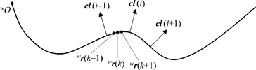
Figure 3.2 Relation between CL data cl(i) and desired trajectory wr(k), in which wO is the origin of work coordinate system.
so that each component of vt in work coordinate system is obtained by
Using a sampling width ∆t, each component of the desired position wxd(k) is represented by
Next, how to calculate the desired orientation od(k) is considered. By using the orientation components of two adjacent steps in CL data, a rotational direction vector tr(i) = [trx(i) try(i) trz(i)]T is defined as
Each component of desired orientation can be linearly calculated with tr(i) as
wxd(k) and wod(k) shown above are directly obtained from the CL data without either any conventional complicated teaching process or recently proposed off-line teaching methods. The desired position and orientation in the discrete-time domain are very important to control the tip of an industrial robot in real time, i.e., to design a feedback control system.
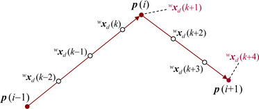
If the linear approximation is applied when CL data are generated by the main-processor of CAD/CAM, CL data forming a curved line are composed of continuous minute lines such as || p(i) – p(i – 1)||and ||p(i + 1) – p(i)|| shown in Fig. 3.3. In this case, it should be noted that each position vector in CL data such as p(i) and p(i + 1) shown in Fig. 3.3 have to be carefully dealt with in order to be accurately followed along the CL data. For example, wxd(k + 1) and wxd(k + 4) are not calculated by using Eqs. (3.6), (3.7) and (3.8) but have to be directly set with p(i) and p(i + 1), respectively, just before the feed direction changes. ||p(i) – wxd(k)|| and ||p(i + 1) – wxd(k + 3)|| are called the fraction.
3.3 Implementation to industrial robot RV1A
3.3.1 Communication between PC and robot controller
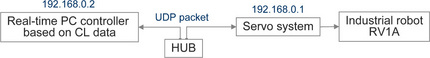
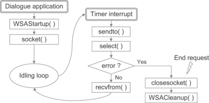
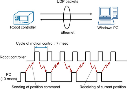
A Windows PC as a controller and the RV1A are connected via Ethernet as shown in Fig. 3.4. The servo system in the Cartesian coordinate system of the RV1A is technically opened to users, so that absolute coordinate vectors of position and orientation can be given to the reference of the servo system. The servo rate of the robot is fixed to 7.1 ms. Fig. 3.5 illustrates the communication scheme by using UDP packet, in which sampling period is set to 10 ms. The data size in a UDP pachet is 196 bytes. The packet transmitted by ‘sendto( )’ includes values of desired position [Xd(k) Yd(k) Zd(k)]T [mm] and desired orientation [ϕd(k) θd(k) ψd(k)]T [rad] in robot absolute coordinate system.ϕd(k), θd(k), ψd(k) are the rotational angles about x-, y- and z-axes, respectively, which are called X-Y-Z fixed angles or roll, pitch and yaw angles. The desired position and the desired orientation are set in a UDP packet as the reference of the arm tip in the Cartesian servo system. Moreover, the packet received by ‘recvfrom( )’ includes values of current position [X(k) Y(k) Z(k)]T [mm] and current orientation [ϕ(k) θ(k) ψ(k)]T [rad] in robot absolute coordinate system, which can be used for feedback quantity.
3.3.2 Desired position and orientation for arm tip
In this subsection, the making of [Xd(k) Yd(k) Zd(k)]T and [ϕd(k) θd(k) ψd(k)]T based on the position and the orientation given by Eq. (3.1) is discussed in detail by using an example shown in Fig. 3.2, in which the tip of robot arm follows the trajectory, keeping the orientation along the normal direction to the surface. Each component of [Xd(k) Yd(k) Zd(k)]T is represented with the initial position [Xd(0) Yd(0) Zd(0)]T as
where [Xd(0) Yd(0) Zd(0)]T means the values of wO in robot absolute coordinate system.
Next, we consider the rotational components. Generally, rotational matrices RX, RY and RZ around x-, y- and z-axes are given by

Accordingly, the rotational matrix RZ RY RX with a roll angle ϕ(k), a pitch angle θ(k), and a yaw angle ψ(k) is given by
where, for example, Sθ and Cθ means sin θ(k) and cos θ(k), respectively. Fig. 3.6 illustrates the trajectory following control along CL data shown in Fig. 3.2. As can be seen, the direction of wod(k) is just inverse to the one of the arm tip. When referring the orientation components in CL data, the arm tip can be determined only with the roll angle and the pitch angle except for the yaw angle. That means ψ(k) can be always fixed to 0 [rad]. Thus, Eq. (3.17) is simplified by giving 0 to ψ(k) as
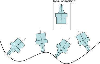
Figure 3.6 Orientation control of arm tip based on CL data shown in Fig. 3.2, in which the initial orientation is given with [ϕ(k) θ(k) ψ(k)]T = [0 0 0]T.
The roll angle ϕ(k) and the pitch angle θ(k) at the discrete time k are obtained by solving
where [0 0 1]T is the initial orientation vector in robot absolute coordinate system as shown in Fig. 3.6. Finally, ϕ(k) and θ(k) are calculated by using inverse trigonometric functions as
If the yaw angle is always fixed to 0, then the desired roll angle ϕd(k) and pitch angle θd(k) at the discrete time k can be calculated with Eqs. (3.20) and (3.21), respectively.
3.4 Experiment
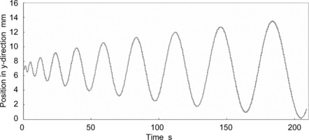
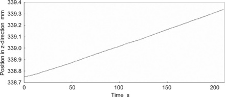
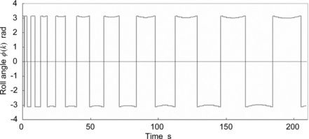
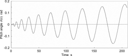
In this section, an experiment of trajectory following control is conducted to evaluate the effectiveness of the proposed CAM system. Fig. 3.7 shows the desired trajectory generated by using the main-processor of 3D CAD/CAM Pro/Engineer, which consists of position and orientation components written by multi-lined ”GOTO/” statements. In this experiment, it is tried that the arm tip is controlled so as to follow the position and orientation. Figs. 3.8, 3.9 and 3.10 show the initial parts of x-component Xd(k), y-component Yd(k) and z-component Zd(k) of the desired trajectory in robot absolute coordinate system, respectively. Moreover, Figs. 3.11 and 3.12 show the initial parts of the roll angle ϕd(k) and the pitch angle θd(k), respectively, of the desired trajectory in the robot absolute coordinate system. In the trajectory following control experiments, the value of feed rate, i.e., tangential velocity, is set to 1 mm/s; the desired values composed of Xd(k), Yd(k), Zd(k), ϕd(k), θd(k) and ψd(k) are given to the references of the servo controller of RV1A every sampling period with UDP packets.
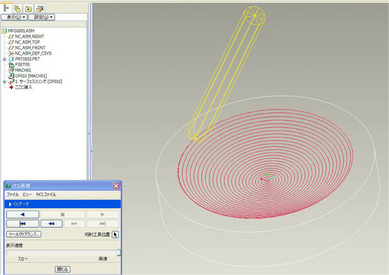
Figure 3.7 CL data cl(i) = [pT(i) nT(i)]T consisting of position and orientation components, which is used for desired trajectory of the tip of robot arm.
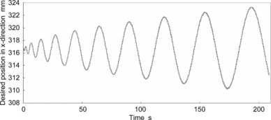
Figure 3.8 Initial part of x-component Xd(k) of desired trajectory in robot absolute coordinate system.
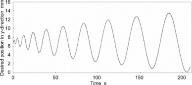
Figure 3.9 Initial part of y-component Yd(k) of desired trajectory in robot absolute coordinate system.
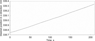
Figure 3.10 Initial part of z-component Zd(k) of desired trajectory in robot absolute coordinate system.
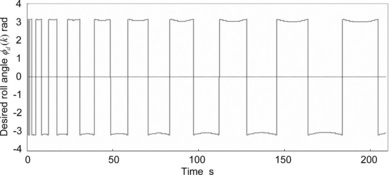
Figure 3.11 Initial part of desired roll angle ϕd(k) calculated from the desired trajectory shown in Fig. 3.7.
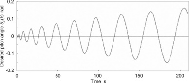
Figure 3.12 Initial part of desired pitch angle θd(k) calculated from the desired trajectory shown in Fig. 3.7.
When the desired position [Xd(k) Yd(k) Zd(k)]T and orientation [ϕd(k) θd(k) ψd(k)]T is transmitted to the robotic servo system, the roll angle ϕd(k) has to be given within the range from –π to π. Fig. 3.13 shows four examples of roll angle around x-axis, in which (a) is the initial angle represented by ϕ(k) = 0, (b) is the case of –π ≤ ϕ(k) < 0, (c) is the case of ϕ(k) = ± π, and (d) is the case of 0 < ϕ(k) ≤ π. It should be noted how to calculate the desired roll angle ϕd(k) as an manipulated value if the orientation changes as (b) → (c) → (d) or (d) → (c) → (b), i.e., in passing through the situation (c). In such cases, the sign of ϕd(k) has to be suddenly changed as shown in Fig. 3.11. In order to smoothly control the orientation of the arm tip, the following control rules were applied for the correction of roll angle.
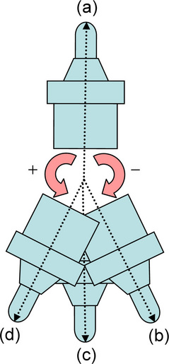
Figure 3.13 Roll angles around x-axis, in which (a) is the initial angle represented by (k) = 0, (b) is the case of − π ≤ ϕ(k) < 0, (c) is the case of ϕ(k) = ± π, and (d) is the case of 0 < ϕ(k) ≤ π.
where ϕd(k) and ϕ(k) are the desired roll angle transmitted to the robotic servo controller and actual roll angle transmitted from the robotic servo controller, respectively. ∆ϕ(k) is the output of proportional control action with a gain Kp. In fact, the desired roll angle ϕd(k + 1) is generated as
Figs. 3.14, 3.15, 3.16, 3.17 and 3.18 show the actual results controlled based on the references shown in Figs. 3.8, 3.9, 3.10, 3.11 and 3.12, respectively. It was confirmed from the experiment that the desired control results of position and orientation could be obtained. The arm tip could gradually move up from the bottom center along the spiral path shown in Fig. 3.7. In this case, the orientation of the arm tip was simultaneously controlled so as to be in a normal direction to the surface. It was successfully demonstrated that the proposed CAM system allows the tip of the robot arm to desirably follow the desired trajectory given by multi-axis CL data without any complicated teaching tasks.
3.5 Passive force control of industrial robot RV1A
3.5.1 Derivation of passive force control laws by using a inner servo system
In this subsection, passive force control methods of the industrial robot are introduced. They are called stiffness control, compliance control and impedance control. The relative position vector ∆x is written by
where xd and x are the desired position and current position vectors, respectively. Kp = diag(Kpx, Kpy, Kpz) is the position feedback gain. ∆x is the manipulated variable from the outer position control system to the technically-opened high-rate servo system in the robot controller.
First of all, a stiffness control is simply considered. The desired stiffness model is designed by
where Kd = diag(Kdx, Kdy, Kdz) is the desired stiffness, F is the external force given to the arm tip. x0 is the initial position in the case of F = 0. Eq. (3.25) is represented with x as
Eq. (3.26) is substituted into xd in Eq. (3.24) to realize a stiffness control by using the servo system, so that the following equation is obtained.
Next, a compliance control is also considered, in which the velocity is further controlled according to the external force. The desired compliance model is designed by
where Bd = diag(Bdx, Bdy, Bdz) is the desired damping, ![]() and
and ![]() are the initial velocity and current velocity, respectively. As can be seen, Eq. (3.28) is regarded as a first-order lag system. When F is constantly given, the following step response in time domain is obtained by solving Eq. (3.28) under the condition of
are the initial velocity and current velocity, respectively. As can be seen, Eq. (3.28) is regarded as a first-order lag system. When F is constantly given, the following step response in time domain is obtained by solving Eq. (3.28) under the condition of ![]() = 0.
= 0.
where I is the identity matrix. The external force F is absorbed by Eq. (3.29). Eq. (3.29) is substituted into xd in Eq. (3.24) to realize a compliance control by using the inner servo system. The relative position command to perform the compliance control is given by
When an impedance control is applied, the acceleration is further controlled. The desired impedance model is designed by
where Md = diag(Mdx, Mdy, Mdz) is the desired mass, ![]() and
and ![]() are the initial acceleration and current acceleration, respectively. Solving Eq. (3.31) under the condition of damping coefficients ζi < 1 (i = x, y, z),
are the initial acceleration and current acceleration, respectively. Solving Eq. (3.31) under the condition of damping coefficients ζi < 1 (i = x, y, z), ![]() and
and ![]() = 0, the following response in time domain is obtained.
= 0, the following response in time domain is obtained.
where the damping coefficient matrix ζ = diag(ζx, ζy, ζz) and natural frequency matrix ωn = diag(ωnx, ωny, ωnz) are given by
By substituting Eq. (3.32) into xd in Eq. (3.24), an impedance control can be easily realized by using the servo system as
3.5.2 Experiments of passive force controllers
As the first case study, the stiffness control law given by Eq. (3.27) is applied. In the experiment on stiffness control, a student is pulling the force sensor attached to the arm tip with 10 N as shown in Fig. 3.20. Fig. 3.21 shows the experimental results when Eq. (3.27) is used in x-direction with several desired stiffnesses Kdx N/mm, where the relations between the time and the position are plotted. As can be seen, the mechanical stiffness is controlled according to the desired stiffness.
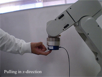
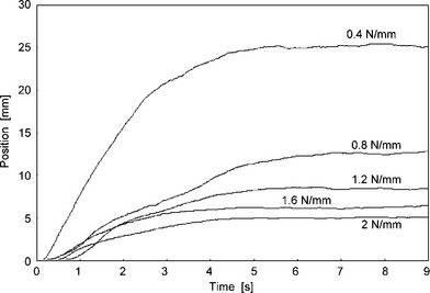
Figure 3.21 Experimental results when Eq. (3.27) is used in x-direction with several desired stiffness Kdx N/mm. The relations between the time and position are plotted.
As the second case study, the compliance control law given by Eq. (3.30) is applied. In this case, the mechanical damping and stiffness in x-direction can be regulated by changing Bdx and Kdx, respectively. Fig. 3.22 shows experimental results when Eq. (3.30) is used in x-direction with several desired damping Bdx Ns/mm, in which the relations between the time and position are plotted. It is observed that the mechanical damping is successfully varied according to the desired damping. Note that the Kdx is set to a constant value of 0.4 N/mm.

Figure 3.22 Experimental results when Eq. (3.30) is used in x-direction with several desired dampings Bdx Ns/mm. The relations between the time and position are plotted.
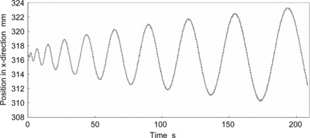
As the third case study, the impedance control law given by Eq. (3.32) is used. In this case, the mechanical impedance in x-direction can be regulated by changing the damping coefficient ζ. Fig. 3.23 shows experimental results when Eq. (3.32) is used in x-direction with several damping coefficients ζ, in which the relations between the time and the position are plotted. It is observed that the mechanical impedance is also successfully varied according to the damping coefficient. Note that the Kdx is also set to a constant value of 0.4 N/mm.
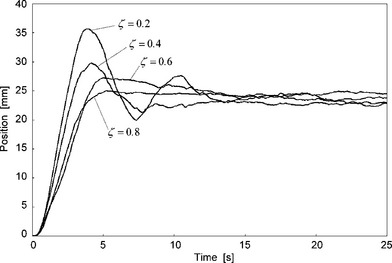
Figure 3.23 Experimental results when Eq. (3.32) is used in x-direction with several damping cofficients ζ. The relations between the time and position are plotted.
3.6 Conclusion
In this chapter, a CAM system for an articulated-type industrial robot RV1A has been proposed in order to improve the relationship between a design tool such as CAD/CAM and industrial robots spread across industrial manufacturing fields. A simple and flexible CAM system has been proposed from the viewpoint of cooperation between CL data and robotic servo system. The CAM system required for an industrial robot is realized as an integrated system including not only a conventional main-processor of CAM but also a robotic servo system and kinematics. Basic design of the CAM system and experimental results have been shown using the desktop-size industrial robot RV1A. The effectiveness has been demonstrated through a trajectory following control along multi-axis CL data consisting position and orientation components. In future work, we plan to develop a 3D carving machine for wooden materials based on an industrial robot, in which the concept of the proposed CAM system will be incorporated as an important interface between CAD/CAM and the industrial robot.
Then, passive force control methods called stiffness control, compliance control and impedance control were proposed and also the controllers were designed using the robotic inner servo system of the RV1A. It was successfully demonstrated that the industrial robot RV1A could perform desired compliance against an external force.
References
[1] Chen, C., Trivedi, M.M., Bidlack, C.R. Simulation and animation of sensor-driven robots. IEEE Trans. on Robotics and Automation. 1994; 10(5):684–704.
[2] Benimeli, F., Mata, V., Valero, F. A comparison between direct and indirect dynamic parameter identification methods in industrial robots. Robotica. 2006; 24(5):579–590.
[3] Corke, P. A Robotics Toolbox for MATLAB. IEEE Robotics & Automation Magazine. 1996; 3(1):24–32.
[4] Corke, P. MATLAB Toolboxes: robotics and vision for students and teachers. IEEE Robotics & Automation Magazine. 2007; 14(4):16–17.
[5] Luh, J.Y.S., Walker, M.H., Paul, R.P.C. Resolved acceleration control of mechanical manipulator. IEEE Trans. on Automatic Control. 1980; 25(3):468–474.
[6] Nagata, F., Kuribayashi, K., Kiguchi, K., Watanabe, K. Simulation of fine gain tuning using genetic algorithms for model-based robotic servo controllers. IEEE International Symposium on Computational Intelligence in Robotics and Automation. (196–201):2007.
[7] Nagata, F., Okabayashi, I., Matsuno, M., Utsumi, T., Kuribayashi, K., Watanabe, K., Fine gain tuning for model-based robotic servo controllers using genetic algorithms. 13th International Conference on Advanced Robotics. 2007:987–992.
[8] Hogan, N. Impedance control: An approach to manipulation: Part I - Part III. Transactions of the ASME, Journal of Dynamic Systems, Measurement and Control. 1985; 107:1–24.
[9] Nagata, F., Watanabe, K., Hashino, S., Tanaka, H., Matsuyama, T., Hara, K., Polishing robot using a joystick controlled teaching system. IEEE International Conference on Industrial Electronics, Control and Instrumentation. 2000:632–637.
[10] Craig, J.J. Introduction to ROBOTICS —Mechanics and Control Second Edition—. Addison Wesley Publishing Co., Reading, Mass; 1989.
[11] Nagata, F., Kusumoto, Y., Fujimoto, Y., Watanabe, K. Robotic sanding system for new designed furniture with free-formed surface. Robotics and Computer-Integrated Manufacturing. 2007; 23(4):371–379.
[12] Kawato, M. The feedback-error-learning neural network for supervised motor learning. In: Advanced Neural Computers. Elsevier Amsterdam; 1990:365–373.
[13] Nakanishi, J., Schaal, S. Feedback error learning and nonlinear adaptive control. Neural Networks. 2004; 17(10):1453–1465.
[14] Furuhashi, T., Nakaoka, K., Maeda, H., Uchikawa, Y. A proposal of genetic algorithm with a local improvement mechanism and finding of fuzzy rules. Journal of Japan Society for Fuzzy Theory and Systems. 1995; 7(5):978–987. [(in Japanese)].
[15] Linkens, D.A., Nyongesa, H.O. Genetic algorithms for fuzzy control part 1: Offline system development and application. IEE Proceedings Control Theory and Applications. 1995; 142(3):161–176.
[16] Linkens, D.A., Nyongesa, H.O. Genetic algorithms for fuzzy control part 2: Online System Development and Application. IEE Proceedings Control Theory and Applications. 1995; 142(3):177–185.
[17] Ferretti, G., Magnani, G., Zavala Rio, A. Impact modeling and control for industrial manipulators. IEEE Control Systems Magazine. 1998; 18(4):65–71.
[18] Sasaki, T., Tachi, S. Contact stability analysis on some impedance control methods. Journal of the Robotics Society of Japan. 1994; 12(3):489–496. [(in Japanese)].
[19] An, H.C., Hollerbach, J.M., Dynamic stability issues in force control of manipulators. IEEE International Conference on Robotics and Automation. 1987:890–896.
[20] An, H.C., Atkeson, C.G., Hollerbach, J.M., Model-based control of a robot manipulatorThe MIT Press classics series. Massachusetts: The MIT Press, 1988.
[21] Takagi, T., Sugeno, M. Fuzzy identification of systems and its applications to modeling and control. IEEE Transactions Systems, Man & Cybernetics. 1985; 15(1):116–132.
[22] Nagata, F., Watanabe, K., Sato, K., Izumi, K., An experiment on profiling task with impedance controlled manipulator using cutter location data. IEEE International Conference on Systems, Man, and Cybernetics. 1999:848–853.
[23] Nagata, F., Watanabe, K., Izumi, K., Furniture polishing robot using a trajectory generator based on cutter location data. IEEE International Conference on Robotics and Automation. 2001:319–324.
[24] Raibert, M.H., Craig, J.J. Hybrid position/force control of manipulators. Transactions of the ASME, Journal of Dynamic Systems, Measurement and Control. 1981; 102:126–133.
[25] Nagata, F., Hase, T., Haga, Z., Omoto, M., Watanabe, K. CAD/CAM-based position/force controller for a mold polishing robot. Mechatronics. 2007; 17(4/5):207–216.
[26] Nagata, F., Watanabe, K., Hashino, S., Tanaka, H., Matsuyama, T., Hara, K. Polishing robot using joystick controlled teaching. Journal of Robotics and Mechatronics. 2001; 13(5):517–525.
[27] Nagata, F., Watanabe, K., Kiguchi, K. Joystick teaching system for industrial robots using fuzzy compliance control. Industrial Robotics: Theory, Modelling and Control, INTECH, pages. (799–812):2006.
[28] Maeda, Y., Ishido, N., Kikuchi, H., Arai, T., Teaching of grasp/graspless manipulation for industrial robots by human demonstration. IEEE/RSJ International Conference on Intelligent Robots and Systems. 2002:1523–1528.
[29] Kushida, D., Nakamura, M., Goto, S., Kyura, N. Human direct teaching of industrial articulated robot arms based on force-free control. Artificial Life and Robotics. 2001; 5(1):26–32.
[30] Sugita, S., Itaya, T., Takeuchi, Y. Development of robot teaching support devices to automate deburring and finishing works in casting. The International Journal of Advanced Manufacturing Technology. 2003; 23(3/4):183–189.
[31] Ahn, C.K., Lee, M.C., An off-line automatic teaching by vision information for robotic assembly task. IEEE International Conference on Industrial Electronics, Control and Instrumentation. 2000:2171–2176.
[32] Neto, P., Pires, J.N., Moreira, A.P., CAD-based offline robot programming. IEEE International Conference on Robotics Automation and Mechatronics. 2010:516–521.
[33] Ge, D.F., Takeuchi, Y., Asakawa, N. Automation of polishing work by an industrial robot, – 2nd report, automatic generation of collision-free polishing path –. Transaction of the Japan Society of Mechanical Engineers. 1993; 59(561):1574–1580. [(in Japanese)].
[34] Ozaki, F., Jinno, M., Yoshimi, T., Tatsuno, K., Takahashi, M., Kanda, M., Tamada, Y., Nagataki, S. A force controlled finishing robot system with a task-directed robot language. Journal of Robotics and Mechatronics. 1995; 7(5):383–388.
[35] Pfeiffer, F., Bremer, H., Figueiredo, J. Surface polishing with flexible link manipulators. European Journal of Mechanics, A/Solids. 1996; 15(1):137–153.
[36] Takeuchi, Y., Ge, D., Asakawa, N., Automated polishing process with a human-like dexterous robot. IEEE International Conference on Robotics and Automation. 1993:950–956.
[37] Pagilla, P.R., Yu, B. Robotic surface finishing processes: modeling, control, and experiments. Transactions of the ASME, Journal of Dynamic Systems, Measurement and Control. 2001; 123:93–102.
[38] Huang, H., Zhou, L., Chen, X.Q., Gong, Z.M. SMART robotic system for 3D profile turbine vane airfoil repair. International Journal of Advanced Manufacturing Technology. 2003; 21(4):275–283.
[39] Stephien, T.M., Sweet, L.M., Good, M.C., Tomizuka, M. Control of tool/workpiece contact force with application to robotic deburring. IEEE Journal of Robotics and Automation. 1987; 3(1):7–18.
[40] Kazerooni, H. Robotic deburring of two-dimensional parts with unknown geometry. Journal of Manufacturing Systems. 1988; 7(4):329–338.
[41] Her, M.G., Kazerooni, H. Automated robotic deburring of parts using compliance control. Transactions of the ASME, Journal of Dynamic Systems, Measurement and Control. 1991; 113:60–66.
[42] Bone, G.M., Elbestawi, M.A., Lingarkar, R., Liu, L. Force control of robotic deburring. Transactions of the ASME, Journal of Dynamic Systems, Measurement and Control. 1991; 113:395–400.
[43] Gorinevsky, D.M., Formalsky, A.M., Schneider, A.Y. Force Control of Robotics Systems. New York: CRC Press; 1997.
[44] Takahashi, K., Aoyagi, S., Takano, M., Study on a fast profiling task of a robot with force control using feedforward of predicted contact position data. 4th Japan-France Congress & 2nd Asia-Europe Congress on Mechatronics. 1998:398–401.
[45] Takeuchi, Y., Watanabe, T. Study on post-processor for 5-axis control machining. Journal of the Japan Society for Precision Engineering. 1992; 58(9):1586–1592. [(in Japanese)].
[46] Takeuchi, Y., Wada, K., Hisaki, T., Yokoyama, M. Study on post-processor for 5-axis control machining centers —In case of spindle-tilting type and table/spindle-tilting type. Journal of the Japan Society for Precision Engineering. 1994; 60(1):75–79. [(in Japanese)].
[47] Xu, X.J., Bradley, C., Zhang, Y.F., Loh, H.T., Wong, Y.S. Tool-path generation for five-axis machining of free-form surfaces based on accessibility analysis. International Journal of Production Research. 2002; 40(14):3253–3274.
[48] Chen, S.L., Chang, T.H., Inasaki, I., Liu, Y.C. Postprocessor development of a hybrid TRR-XY parallel kinematic machine tool. The International Journal of Advanced Manufacturing Technology. 2002; 20(4):259–269.
[49] Lei, W.T., Hsu, Y.Y. Accuracy test of five-axis CNC machine tool with 3D probe-ball Part I: design and modeling. Machine Tool & Manufacture. 2002; 42(10):1153–1162.
[50] Lei, W.T., Sung, M.P., Liu, W.L., Chuang, Y.C. Double ballbar test for the rotary axes of five-axis CNC machine tools. Machine Tool & Manufacture. 2006; 47(2):273–285.
[51] Cao, L.X., Gong, H., Liu, J. The offset approach of machining free form surface. Part 1: Cylindrical cutter in five-axis NC machine tools. Journal of Materials Processing Technology. 2006; 174(1/3):298–304.
[52] Cao, L.X., Gong, H., Liu, J. The offset approach of machining free form surface. Part 2: Toroidal cutter in 5-axis NC machine tools. Journal of Materials Processing Technology. 2007; 184(1/3):6–11.
[53] Timar, S.D., Farouki, R.T., Smith, T.S., Boyadjieff, C.L. Algorithms for time optimal control of CNC machines along curved tool paths. Robotics and Computer-Integrated Manufacturing. 2005; 21(1):37–53.
[54] Heo, E.Y., Kim, D.W., Kim, B.H., Chen, F.F. Estimation of NC machining time using NC block distribution for sculptured surface machining. Robotics and Computer-Integrated Manufacturing. 2006; 22(5–6):437–446.
[55] Tarng, Y.S., Chuang, H.Y., Hsu, W.T. Intelligent cross-coupled fuzzy feedrate controller design for CNC machine tools based on genetic algorithms. International Journal of Machine Tools and Manufacture. 1999; 39(10):1673–1692.
[56] Zuperl, U., Cus, F., Milfelner, M. Fuzzy control strategy for an adaptive force control in end-milling. Journal of Materials Processing Technology. 2005; 164/165:1472–1478.
[57] Farouki, R.T., Manjunathaiah, J., Nicholas, D., Yuan, G.F., Jee, S. Variable-feedrate CNC interpolators for constant material removal rates along Pythagorean-hodograph curves. Computer-Aided Design. 1998; 30(8):631–640.
[58] Farouki, R.T., Manjunathaiah, J., Yuan, G.F. G codes for the specification of Pythagorean-hodograph tool paths and associated feedrate functions on open-architecture CNC machines. Machine Tools & Manufacture. 1999; 39(1):123–142.
[59] Frank, A., Schmid, A. Grinding of non-circular contours on CNC cylindrical grinding machines. Robotics and Computer-Integrated Manufacturing. 1988; 4(1/2):211–218.
[60] Couey, J.A., Marsh, E.R., Knapp, B.R., Vallance, R.R. Monitoring force in precision cylindrical grinding. Precision Engineering. 2005; 29(3):307–314.
[61] Tawakoli, T., Rasifard, A., Rabiey, M. Highefficiency internal cylindrical grinding with a new kinematic. Machine Tools & Manufacture. 2007; 47(5):729–733.
[62] Nagata, F., Kusumoto, Y., Hasebe, K., Saito, K., Fukumoto, M., Watanabe, K., Post-processor using a fuzzy feed rate generator for multi-axis NC machine tools with a rotary unit. International Conference on Control, Automation and Systems. 2005:438–443.
[63] Nagata, F., Watanabe, K. Development of a postprocessor module of 5-axis control NC machine tool with tilting-head for woody furniture. Journal of the Japan Society for Precision Engineering. 1996; 62(8):1203–1207. [(in Japanese)].
[64] Fujino, K., Sawada, Y., Fujii, Y., Okumura, S., Machining of curved surface of wood by ball end mill – Effect of rake angle and feed speed on machined surface. 16th International Wood Machining Seminar, Part 2. 2003:532–538.
[65] Nagata, F., Hase, T., Haga, Z., Omoto, M., Watanabe, K., Intelligent desktop NC machine tool with compliance control capability. 13th International Symposium on Artificial Life and Robotics. 2008:779–782.
[66] Duffy, J. The Fallacy of modern hybrid control theory that is based on orthogonal complements of twist and wrench spaces. Journal of Robotic Systems. 1990; 7(2):139–144.
[67] Lee, M.C., Go, S.J., Lee, M.H., Jun, C.S., Kim, D.S., Cha, K.D., Ahn, J.H. A robust trajectory tracking control of a polishing robot system based on CAM data. Robotics and Computer-Integrated Manufacturing. 2001; 17(1/2):177–183.
[68] Nagata, F., Mizobuchi, T., Tani, S., Hase, T., Haga, Z., Watanabe, K., Habib, M.K., Kiguchi, K., Desktop orthogonal-type robot with abilities of compliant motion and stick-slip motion for lapping of LED lens molds. IEEE International Conference on Robotics & Automation. 2010:2095–2100.
[69] Bilkay, O., Anlagan, O. Computer simulation of stick-slip motion in machine tool slideways. Tribology International. 2004; 37(4):347–351.
[70] Mei, X., Tsutsumi, M., Tao, T., Sun, N. Study on the compensation of error by stick-slip for high-precision table. International Journal of Machine tools & Manufacture. 2004; 44(5):503–510.
[71] Tsai, M.J., Chang, J.L., Haung, J.F., Development of an automatic mold polishing system. IEEE International Conference on Robotics & Automation. 2003:3517–3522.
[72] Tsai, M.J., Fang, J.J., Chang, J.L. Robotic path planning for an automatic mold polishing system. International Journal of Robotics & Automation. 2004; 19(2):81–89.
[73] Hocheng, H., Sun, Y.H., Lin, S.C., Kao, P.S. A material removal analysis of electrochemical machining using flat-end cathode. Journal of Materials Processing Technology. 2003; 140(1/3):264–268.
[74] Uehara, Y., Ohmori, H., Lin, W., Ueno, Y., Naruse, T., Mitsuishi, N., Ishikawa, S., Miura, T., Development of spherical lens ELID grinding system by desk-top 4-axes Machine Tool. International Conference on Leading Edge Manufacturing in 21st Century. 2005:247–252.
[75] Ohmori, H., Uehara, Y. Development of a desktop machine tool for mirror surface grinding. International Journal of Automation Technology. 2010; 4(2):88–96.
[76] Nagata, F., Hase, T., Haga, Z., Omoto, M., Watanabe, K. Intelligent desktop NC machine tool with compliant motion capability. Artificial Life and Robotics. 2009; 13(2):423–427.
[77] Nagata, F., Tani, S., Mizobuchi, T., Hase, T., Haga, Z., Omoto, M., Watanabe, K., Habib, M.K., Basic performance of a desktop NC machine tool with compliant motion capability. IEEE International Conference on Mechatronics and Automation, WC1-5. 2008:1–6.
[78] Nagata, F., Watanabe, K., Sato, K., Izumi, K. Impedance control using anisotropic fuzzy environment models. Journal of Robotics and Mechatronics. 1999; 11(1):60–66.
[79] Nagata, F., Otsuka, A., Yoshitake, S., Watanabe, K., Automatic control of an orthogonal-type robot with a force sensor and a small force input device. The 37th Annual Conference of the IEEE Industrial Electronics Society. 2011:3151–3156.
[80] Nagata, F., Watanabe, K. Feed rate control using a fuzzy reasoning for a mold polishing robot. Journal of Robotics and Mechatronics. 2006; 18(1):76–82.
[81] Nagata, F., Watanabe, K., Japanese Patent 4094781, Robotic force control method, 2008.
[82] Nagata, F., Tsuda, K., Watanabe, K., Japanese Patent 4447746, Robotic trajectory teaching method, 2010.
[83] Tsuda, K., Yasuda, K., Nagata, F., Kusumoto, Y., Watanabe, K., Japanese Patent 4216557, Polishing apparatus and polishing method, 2008.